1. Chapter 6 : Calculus
06-01 Limits
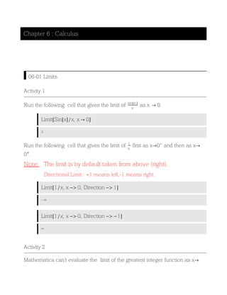
Activity 1
Run the following cell that gives the limit of sin x
x
as x 0.
Limit Sin x x, x 0
1
Run the following cell that gives the limit of 1
x
first as x 0 and then as x
0 .
Note: The limit is by default taken from above (right).
Directional Limit : +1 means left,-1 means right.
Limit 1 x, x 0, Direction 1
Limit 1 x, x 0, Direction 1
Activity 2
Mathematica can't evaluate the limit of the greatest integer function as x
1 . Run the following cell.
2. Mathematica can't evaluate the limit of the greatest integer function as x
1 . Run the following cell.
Limit Floor x , x 1, Direction 1
0
The limit of a function that is defined by several rules can't be evaluated
directly. Run the following cell and comment on the results.
Clear f, a, b, c, d ;
f x_ : If x 4, 3 x 2, 2 7 x^2 ;
a Limit f x , x 1
b Limit f x , x 7
c Limit f x , x 4, Direction 1
d Limit f x , x 4, Direction 1
5
19
110
10
Try to run the following code to overcome this difficulty.
2 Chapter 6..Calculus .nb
3. fup4 x_ : 3 x 2;
fbelow4 x_ : 2 7 x^2;
a Limit fbelow4 x , x 1
b Limit fup4 x , x 7
c Limit fup4 x , x 4
d Limit fbelow4 x , x 4
5
19
10
110
06-02 Differentiation
Mathematica Commands for Differentiation Operations.
Activity 3
Run the following cell that gives x
x n
.
D[x^n, x]
n x 1 n
Run the following cell that gives the first three derivatives of f x x n
Chapter 6..Calculus .nb 3
4. f x_ : xn
f' x
f'' x
f''' x
n x 1 n
1 n n x 2 n
2 n 1 n n x 3 n
Activity 4
Run the following cell that gives the partial derivative x
x 2
y 2
. y is
assumed to be independent of x.
Clear[x,y,f]
f=x^2 + y^2;
D[f, x]
2 x
Run the following cells. Any of them gives the mixed derivative of
f(x,y)=sin(xy) .
D D Sin x y , x , y
Cos x y x y Sin x y
D Sin x y , x, y
Cos x y x y Sin x y
4 Chapter 6..Calculus .nb
5. x,y Sin x y
Cos x y x y Sin x y
Total Derivative
Activity 5
Run the following cell that gives the total differential of f(x,y) = x 2
y 3
, i.e. it
gives fx dx + fy dy.
Note: Dt[x] denotes dx and Dt[y] denotes dy
Dt x2
y3
2 x y3
Dt x 3 x2
y2
Dt y
Local Minimum and Maximum values of a function
Ask Mathematica about the commands "FindMaximum" and "FindMinimum"
?? FindMaximum
FindMaximum f, x, x0 searches for a
local maximum in f, starting from the point x x0.
FindMaximum f, x, x0 , y, y0 , ... searches for a
local maximum in a function of several variables. More…
Attributes FindMaximum HoldAll, Protected
Options FindMaximum AccuracyGoal Automatic,
Compiled True, EvaluationMonitor None, Gradient Automatic,
MaxIterations 100, Method Automatic, PrecisionGoal Automatic,
StepMonitor None, WorkingPrecision MachinePrecision
Chapter 6..Calculus .nb 5
6. ?? FindMinimum
FindMinimum f, x, x0 searches for a
local minimum in f, starting from the point x x0.
FindMinimum f, x, x0 , y, y0 , ... searches for a
local minimum in a function of several variables. More…
Attributes FindMinimum HoldAll, Protected
Options FindMinimum AccuracyGoal Automatic,
Compiled True, EvaluationMonitor None, Gradient Automatic,
MaxIterations 100, Method Automatic, PrecisionGoal Automatic,
StepMonitor None, WorkingPrecision MachinePrecision
Is there a need for two commands? Is one of them enough?
Activity 6
Run the following cell that evaluates the local minimum of f(x)=x 3
+x 2
-3x+5
starting the search from x = 2.
6 Chapter 6..Calculus .nb
7. Clear f, g, x
f x_ : x3
x2
3 x 5
Plot f x , x, 10, 10
FindMinimum f x , x, 2
10 5 5 10
500
500
1000
3.73165, x 0.720759
Activity 7
Note: The maximum value of f(x) occurs at the point x at which -f(x) has a
minimum value.
Study the following code that gives a local maximum of f starting the search
from x = a. Then activate it.
Find a local maximum of f(x)=x 3
+x 2
-3x+5
Solution:
First plot the function is a suitable domain to estimate a starting point for the
search of the maximum. Run the following cell to get the plot.
Chapter 6..Calculus .nb 7
8. Clear f, x
f x_ : x3
x2
3 x 5
Plot f x , x, 10, 10
10 5 5 10
500
500
1000
From this plot one may guess that a local maximum may occur near x = -2.
06-02 Integration
Indefinite Integral
Activity 8
Run the following two cells that give the indefinite integral of f(x) = 1
x4 a4
8 Chapter 6..Calculus .nb
9. Integrate[1/(x^4 - a^4), x]
1
250
ArcTan
5
x
1
500
Log 5 x
1
500
Log 5 x
1
x4
a4
x
1
250
ArcTan
5
x
1
500
Log 5 x
1
500
Log 5 x
Definite Integrals
Activity 9
Run the following two cells that evaluate the definite integral a
b
ln x d x .
Integrate[ Log[x], {x, a, b} ]
24 5 Π 5 Log 5 19 Log 19
a
b
Log x x
24 5 Π 5 Log 5 19 Log 19
Mathematica cannot give a formula for this definite integral 1
3
x x
x . Run the
following cell to check that.
a1=Integrate[ x^x, {x, 1, 3} ]
1
3
xx
x
However, you can still get a numerical result of that integral by running the
following cell.
Chapter 6..Calculus .nb 9
10. However, you can still get a numerical result of that integral by running the
following cell.
N[a1]
13.7251
Integrating Piecewise Functions
Activity 10
Try to run the following cell that attempts to evaluate the Ceiling function
on the interval [0,2], and observe the output.
Integrate Ceiling x2
, x, 0, 2
7 2 3
However, using the Boole function you can evaluate the above integral by
running the following cell.
Integrate Ceiling x2
Boole 0 x 2 , x, ,
7 2 3
Improper integral
Activity 11
The true definite integral 2
2 1
x 2 x is divergent because of the double pole at
x 0. Run the following cell to check that.
10 Chapter 6..Calculus .nb
11. Integrate[1/x^2, {x, -2, 2}]
Integrate::idiv : Integral of
1
x2
does not converge on 2, 2 . More…
2
2 1
x2
x
Run the following cell that tries to evaluate 0
sin a x
x
x .
Integrate[Sin[a x]/x, {x, 0, Infinity}]
Π
2
Note that the If here gives the condition for the integral to be convergent.
Double integral
Activity 12
Run the following cell that the double integral 0
1
0
x
x 2
y 2
dy dx.
Note that the range of the outermost integration variable appears first. The y
integral is done first. Its limits can depend on the value of x.
Integrate[ x^2 + y^2, {x, 0, 1}, {y, 0, x} ]
1
3
Double Integration over Regions
The Boole function is very useful in computing definite double integral over a
given region.
Integrate[f[x] Boole[ ineq], {x, x1, x2}, {y, y1,y2} ] integrates the function f(x)
over the region defined by all points satisfying the inequality inside the rectan-
gle defined by values of x and y.
Note: You can use Integrate[f[x] Boole[ineq],{x,- , },{y,- , }] if you want
Chapter 6..Calculus .nb 11
12. The Boole function is very useful in computing definite double integral over a
given region.
Integrate[f[x] Boole[ ineq], {x, x1, x2}, {y, y1,y2} ] integrates the function f(x)
over the region defined by all points satisfying the inequality inside the rectan-
gle defined by values of x and y.
Note: You can use Integrate[f[x] Boole[ineq],{x,- , },{y,- , }] if you want
Mathematica to select the inter region defined by the inequality.
Activity 13
Run the following cell that integrates x y y 2
over the region R= {(x,y) :
0 x 1 and 0 y 1}.
Integrate x y y2
, x, 0, 1 , y, 0, 1
7
12
Run the following cells . Comment on the obtained results. Write the inte-
grals that have been evaluated..
Integrate Boole x2
y2
1 , x, 1, 1 , y, 1, 1
Π
Integrate Boole x2
y2
1 , x, 0, 1 , y, 0, 1
Π
4
Integrate Boole x2
y2
1 , x, , , y, ,
Π
Run the following cell . Write the integrals that have been evaluated..
12 Chapter 6..Calculus .nb
13. Integrate x2
Boole x2
4 y2
1 Abs y x , y, , ,
x, ,
1
40
2 5 ArcTan 2
06-03 Differential Operations
Note: Some of the following commands are set for spherical coordinates, so
to use them in Cartesian coordinates, we need to run the following cell.
VectorAnalysis`
SetCoordinates Cartesian x, y, z
Cartesian x, y, z
Grad ( f the gradient of the scalar function f)
Activity 14
Run the following cell that computes the f where f x, y, z 5 x2
y3
z4
Clear[x,y,z]
Grad[5 x^2 y^3 z^4, Cartesian[x, y, z]]
10 x y3
z4
, 15 x2
y2
z4
, 20 x2
y3
z3
Curl ( ×f curl of a vector valued function f)
Chapter 6..Calculus .nb 13
14. Curl ( ×f curl of a vector valued function f)
Activity 15
Run the following cell that computes the f where
f x, y, z x2
, sin x y , e 3 zy
Clear f, x, y, z
f x^2, Sin x y , Exp 3 z y ;
Curl f
3 3 y z
z, 0, y Cos x y
Div ( .f divergence of a vector valued function f)
Activity 16
Run the following cell that computes the .f where
f x, y, z x2
, sin x y , e 3 zy
Clear f, x, y, z
f x^2, Sin x y , Exp 3 z y ;
Div f
2 x 3 3 y z
y x Cos x y
14 Chapter 6..Calculus .nb
15. 06-04 Vector Field
Arrow
Activity 17
Run the following cell that plots a vector with starting point (1,2) and end
point (3,5).
Chapter 6..Calculus .nb 15
16. Graphics Arrow 1, 2 , 3, 5
Plot of Vector Field
Activity 18
Run the following cell that plots a vector field components given by sin x
and cos y .
16 Chapter 6..Calculus .nb
20. Needs "VectorFieldPlots`" ;
VectorFieldPlots`GradientFieldPlot3D x y z, x, 1, 1 ,
y, 1, 1 , z, 1, 1
06-05 Power Series
Power Series expansion
Activity 21
Run the following cell that gives a power series expansion of exp(x) around
x = 0, accurate to order x 5
.
20 Chapter 6..Calculus .nb
21. aa=Series[Exp[x], {x, 0, 5}]
1 x
x2
2
x3
6
x4
24
x5
120
O x 6
Run the following cell that turns the previous power series back into an ordi-
nary expression.
Normal[aa]
1 x
x2
2
x3
6
x4
24
x5
120
Run the following cell that gives a power series expansion of exp(x) around
x = 1, accurate to order x 5
.
Series[ Exp[x], {x, 1, 5} ]
x 1
1
2
x 1 2
1
6
x 1 3
1
24
x 1 4
1
120
x 1 5
O x 1 6
Operations on Power Series
Activity 22
Run the following cell that gives 1
1 aa
.
1 / (1 - aa)
1
x
1
2
x
12
x3
720
O x 4
Run the following cell that gives derivative with respect to x of aa.
Chapter 6..Calculus .nb 21
22. D[aa, x]
1 x
x2
2
x3
6
x4
24
O x 5
Run the following cell that integrates aa with respect to x .
Integrate[aa, x]
x
x2
2
x3
6
x4
24
x5
120
x6
720
O x 7
06-07 Laplace Transform
Activity 23
Ask Mathematica about the commands "LaplaceTransform ", and "
InverseLaplaceTransform"
?? LaplaceTransform
LaplaceTransform expr, t, s gives the Laplace transform of expr.
LaplaceTransform expr, t1, t2, ... , s1, s2, ...
gives the multidimensional Laplace transform of expr. More…
Attributes LaplaceTransform Protected, ReadProtected
?? InverseLaplaceTransform
InverseLaplaceTransform expr, s, t gives the inverse
Laplace transform of expr. InverseLaplaceTransform expr,
s1, s2, ... , t1, t2, ... gives the
multidimensional inverse Laplace transform of expr. More…
Attributes InverseLaplaceTransform Protected, ReadProtected
22 Chapter 6..Calculus .nb
23. Mathematica Commands
Activity 24
Run the following cell that computes the Laplace transform of f(t) = t n
using
the Mathematica command LaplaceTransform.
Clear[f,t,L,IL,s,a]
f[t_]:=t^n
L[f_]:=LaplaceTransform[f[t], t, s]
L[f]
s 1 n
Gamma 1 n
Run the following cell that computes the Inverse Laplace transform of the
previous result.
IL[f_]:=InverseLaplaceTransform[L[f], s, t]
IL[f]
tn
Properties of Laplace Transform
Activity 25
Run the following cell that shows that the Laplace transform is a linear
operator.
Chapter 6..Calculus .nb 23
24. Clear f, g, t, s
LaplaceTransform f t g t , t, s
LaplaceTransform f t g t , t, s
LaplaceTransform f t , t, s LaplaceTransform g t , t, s
LaplaceTransform f t , t, s LaplaceTransform g t , t, s
What do you conclude from the above output?
Laplace Transform of nth derivative of a function
Activity 26
Laplace transforms have the property that they turn integration and differentia-
tion into essentially algebraic operations. Run the following cell and com-
ment on the output
f t_ : Sin t ^2
Do Print LaplaceTransform D f t , t, k , t, s , k, 0, 2
2
4 s s3
2
4 s2
4
4 s s3
2 2 s2
4 s s3
Laplace Transform of an Integral
Activity 27
Integration becomes multiplication by 1 s when one does a Laplace trans-
form. Run the following cell and comment on the output.
24 Chapter 6..Calculus .nb
25. Clear f, s, t
f u_ : u Exp u
LaplaceTransform Integrate f u , u, 0, t , t, s
1 s LaplaceTransform f t , t, s
Apart
1
1 s 2
1
1 s
1
s
1
1 s 2 s
1
1 s 2
1
1 s
1
s
Multidimensional Laplace transforms.
Activity 28
Run the following cell that compute a two-dimensional Laplace transform of
f(t,u)= cos(t) eu
LaplaceTransform Cos t Exp u , t, u , s, v
s
1 s2 1 v
06-06 Programming Calculus
Limits
Chapter 6..Calculus .nb 25
26. Limits
Numerical Approach to Limits
Activity 29
Write a code that computes directional limits numerically. Then run it to
activate it.
Run the following cell that calculates the values of f(x)=sin x
x
as x
approaches 0 from right.
f x_ :
Sin x
x
; c 0; dir 1;
numericalapproachtolimits f, c, dir
Right limit of
Sin x
x
as x 0
x f x
Sin x
x
_______________________________
0.001 1.
0.0009 1.
0.0008 1.
0.0007 1.
0.0006 1.
0.0005 1.
0.0004 1.
0.0003 1.
0.0002 1.
0.0001 1.
Graphical Approach
Activity 30
26 Chapter 6..Calculus .nb
27. Activity 30
Write a code that shows directional limits graphically. Then run it to activate
it.
Run the following cell that illustrates the limit of f(x)= x 3
as x approaches 3 .
f x_ : x^3; c 3;
graphicalapproachtolimits f, c
-4 -2 2 4 6 8 10
-50
50
100
150
-4 -2 2 4 6 8 10
-50
50
100
150
Chapter 6..Calculus .nb 27
30. -4 -2 2 4 6 8 10
-50
50
100
150
-4 -2 2 4 6 8 10
-50
50
100
150
(Ε , ∆ ) Approach
Activity 31
Write a code that provides a graphical illustration of Ε and ∆ approach to
limits. Then activate it.
Run the following cell that illustrates the Ε and ∆ approach of limits based
on f(x)=x sin 1
x
as x 0.
f x_ : x Sin 1 x
c 0.; l 0;
analyticapproachtolimits f, c, l
30 Chapter 6..Calculus .nb
31. The relation between Ε and ∆ in the limit definition
Neiborhood of x 0. is 0.1, 0.1 with ∆ 0.1
-0.1 -0.05 0.05 0.1
-0.075
-0.05
-0.025
0.025
0.05
0.01 eps
-0.1 -0.05 0.05 0.1
-0.075
-0.05
-0.025
0.025
0.05
0.009 eps
-0.1 -0.05 0.05 0.1
-0.075
-0.05
-0.025
0.025
0.05
0.008 eps
Chapter 6..Calculus .nb 31
34. -0.1 -0.05 0.05 0.1
-0.075
-0.05
-0.025
0.025
0.05
0.001 eps
Evaluation of ∆ for a given Ε
Activity 32
Write a code that computes ∆ for a given Ε in the definition of limit. Then
activate it.
Run the following cell that computes ∆ if Ε =0.001 that illustrates that the
limx 1x 2
= 1
f x_ : x^2
c 1; epsilon .001;
evaluationofdelta f, c, epsilon
f x x2
c 1
limx c f x 1
Ε 0.001
∆ 0.000499875
Differentiation
34 Chapter 6..Calculus .nb
35. Differentiation
Average of a function
Activity 33
Run the following cell.
Comment on the output.
Write a code that gives the same output.
Clear f, x, a, b
f x_ : Sin x ; a 0; b Pi 2;
average f, a, b
2
Π
Compare derivative and average of a function
Activity 34
Run the following cell.
Comment on the output.
Write a code that gives the same output.
f x_ : Sin x ; x0 Pi; xn Pi;
derivativeandaverage f, x0, xn
Chapter 6..Calculus .nb 35
42. -3 -2 -1 1 2 3
-1
-0.5
0.5
1
-3 -2 -1 1 2 3
-1
-0.5
0.5
1
First Derivative Test for Local Extreme Points
Activity 35
Run the following cell.
Comment on the output.
Write a code that gives the same output.
42 Chapter 6..Calculus .nb
43. Clear f, x
f x_ : x 1 x 2 x 5 ;
Ε 0.01;
extrempoints1 f, Ε
1 The function is f x 5 x 1 x 2 x
2 Its first derivative is f' x
5 x 1 x 5 x 2 x 1 x 2 x
3 The set of values of x such that f has critical points is
1
3
4 37 ,
1
3
4 37
5 Classification of critical points based on second derivative test :
For point number 1 :
1
3
4 37 , 5
1
3
4 37 1
1
3
4 37 2
1
3
4 37
is a maximum point
For point number 2 :
1
3
4 37 , 5
1
3
4 37 1
1
3
4 37 2
1
3
4 37
is a minimum point
Second Derivative Test for Local Extreme Points
Activity 36
Run the following cell.
Comment on the output.
Write a code that gives the same output.
Chapter 6..Calculus .nb 43
44. Clear f, x
f x_ : x 1 x 2 x 5 ;
extrempoints2 f
1 The function is f x 5 x 1 x 2 x
2 Its first derivative is f' x
5 x 1 x 5 x 2 x 1 x 2 x
3 The set of values of x such that f has critical points is
1
3
4 37 ,
1
3
4 37
4 The second derivative of f is f'' x 8 6 x
5 Classification of critical points based on second derivative test :
For point number 1 :
1
3
4 37 , 5
1
3
4 37 1
1
3
4 37 2
1
3
4 37
is a maximum point
For point number 2 :
1
3
4 37 , 5
1
3
4 37 1
1
3
4 37 2
1
3
4 37
is a minimum point
06-08 Evaluation on Calculus
Exercise 1
For each of the following cells:
a) Study the cell and Guess the output.
b) Run the cells.
c) Compare the output with your guess.
d) Write any general comments or remarks.
44 Chapter 6..Calculus .nb
45. Limit[ x Log[x], x -> 0 ]
Limit
x 1
x 1
, x 1
Limit x Sin 1 x , x 0
Limit Abs x 3 , x 3
D Sin x , x, 5
Integrate[x^2 + y^2, {x, 0, a}, {y, 0, b}]
Integrate[x/((x - 1)(x + 2)), x]
x
9 7 x2
x
f x_ :
x2
4
3 x 2 5 x
;
g x_ : Apart f x
g x
g x x
1
1
1 y2
1 y2
x y
Chapter 6..Calculus .nb 45
46. 0
1
0
1
x y y2
x y
0
Π
3
y
Π
3 Sin x
x
x y
Integrate Max x y2
, x2
y Boole x2
y2
1 , x, , ,
y, ,
f t_ : Sin t
LaplaceTransform f t , t, s
InverseLaplaceTransform , s, t
LaplaceTransform t^4 f t , t, s
InverseLaplaceTransform , s, t
Exercise 2
Use Mathematica to evaluate the following
limx 1
x 1
x3
x
,
limh 0
1 h 2
1
h
,
limx
x2
9
2 x 6
,
,
46 Chapter 6..Calculus .nb
47. limx x2
x 1 x2
x ,
limx
ln x
1 ln x
,
limx ln 2 x ln 1 x ,
limx 0 1 x
2
x
0
4
x 16 3 x x,
cos 1
t
t2
t,
x2
ex
x,
x2
2 x 1
2 x3
3 x2
2 x
x,
0
1
x
1
e
x
y
y x,
Chapter 6..Calculus .nb 47
48. 0
1
y2
1
y sin x2
x y,
Exercise 3
Calculate the first and the second
derivatives of each of the following
y x 2 8
4 x3
3
6
,
y
1
sin x sin x
,
y ln x2
ex
,
y 5x tan x
,
Exercise 4
Find the first and the mixed partial derivatives for the following
f x, y x3
ln x y ,
f x, y, z x ey
cos z
Exercise 5
Find the Taylor series expansion of each of the following
1
1 x2
, at x 0,
48 Chapter 6..Calculus .nb