![Getting data from InternetGetting data from Internet
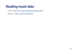
Data from Healthit.gov
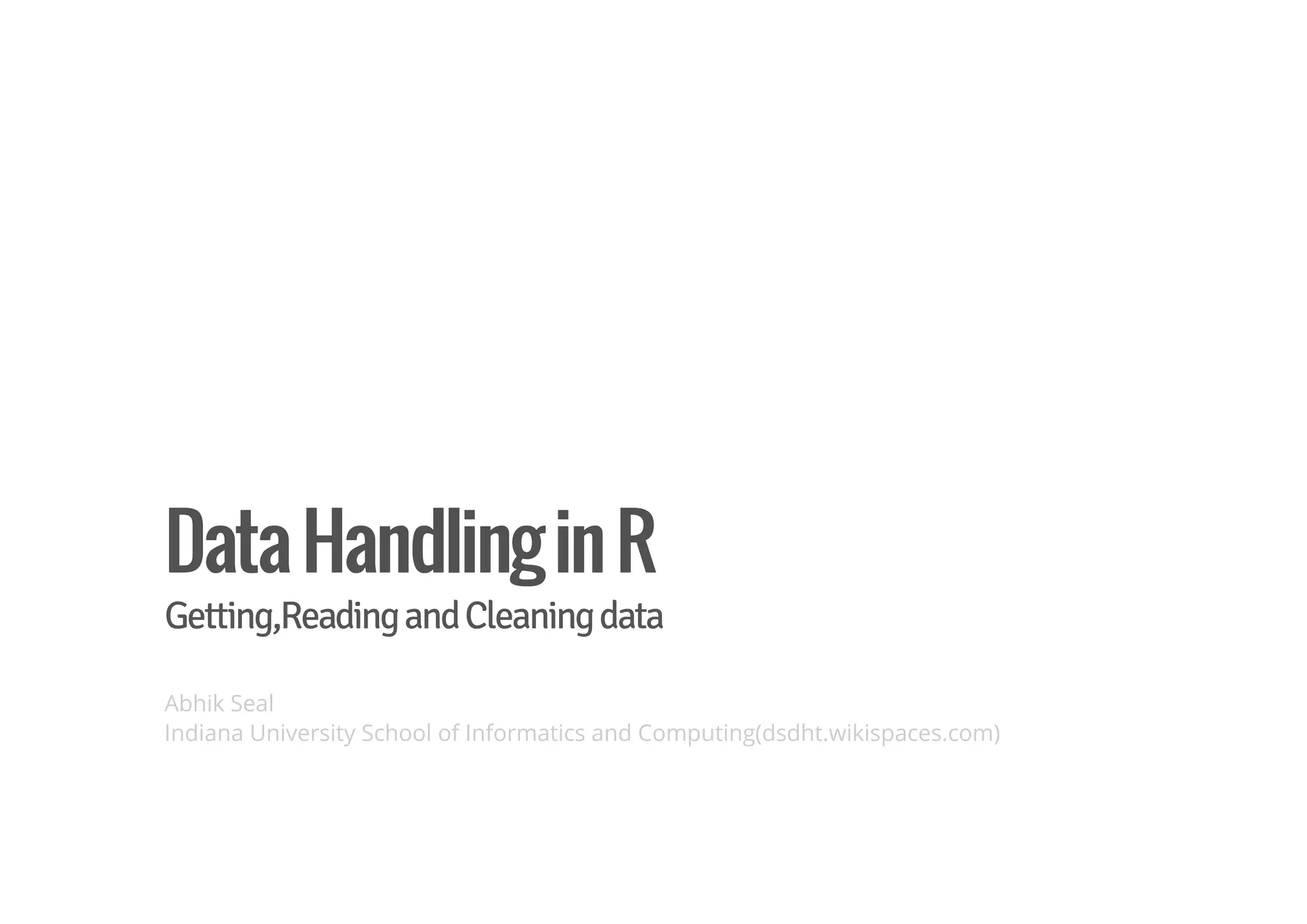
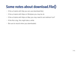
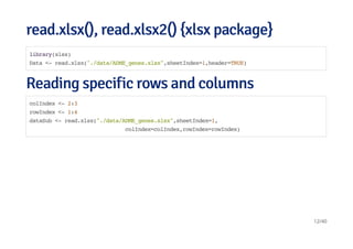
Use of download.file()
Useful for downloading tab-delimited, csv, and other files
·
·
fileUrl <- "http://dashboard.healthit.gov/data/data/NAMCS_2008-2013.csv"
download.file(fileUrl,destfile="./data/NAMCS.csv",method="curl")
list.files("./data")
## [1] "NAMCS.csv"
5/40](https://image.slidesharecdn.com/datahandlinginr-140822100523-phpapp01/85/Data-handling-in-r-5-320.jpg)

![Example dataExample data
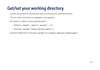
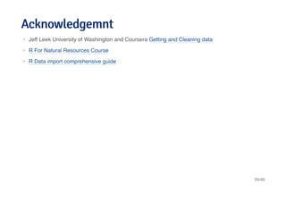
fileUrl <- "http://dashboard.healthit.gov/data/data/NAMCS_2008-2013.csv"
download.file(fileUrl,destfile="./data/NAMCS.csv",method="curl")
list.files("./data")
## [1] "NAMCS.csv"
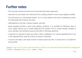
Data <- read.table("./data/NAMCS.csv")
## Error: line 2 did not have 87 elements
head(Data,2)
## Error: object 'Data' not found
9/40](https://image.slidesharecdn.com/datahandlinginr-140822100523-phpapp01/85/Data-handling-in-r-9-320.jpg)
![Read the file into RRead the file into R
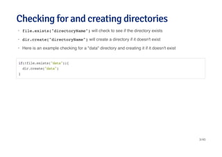
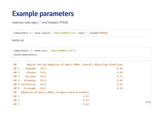
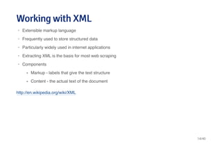
library(XML)
fileUrl <- "http://www.w3schools.com/xml/simple.xml"
doc <- xmlTreeParse(fileUrl,useInternal=TRUE)
rootNode <- xmlRoot(doc)
xmlName(rootNode)
## [1] "breakfast_menu"
names(rootNode)
## food food food food food
## "food" "food" "food" "food" "food"
15/40](https://image.slidesharecdn.com/datahandlinginr-140822100523-phpapp01/85/Data-handling-in-r-15-320.jpg)
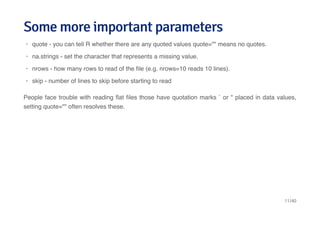
![Directly access parts of the XML documentDirectly access parts of the XML document
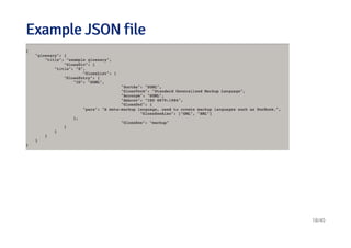
rootNode[[1]]
## <food>
## <name>Belgian Waffles</name>
## <price>$5.95</price>
## <description>Two of our famous Belgian Waffles with plenty of real maple syrup</description>
## <calories>650</calories>
## </food>
rootNode[[1]][[1]]
## <name>Belgian Waffles</name>
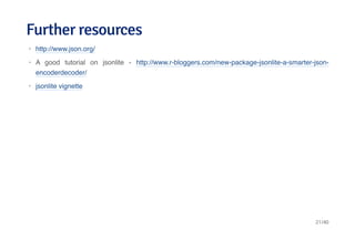
Go for a tour of XML package
Official XML tutorials short, long
An outstanding guide to the XML package
·
·
·
16/40](https://image.slidesharecdn.com/datahandlinginr-140822100523-phpapp01/85/Data-handling-in-r-16-320.jpg)
![JSONJSON
http://en.wikipedia.org/wiki/JSON
Javascript Object Notation
Lightweight data storage
Common format for data from application programming interfaces (APIs)
Similar structure to XML but different syntax/format
Data stored as
·
·
·
·
·
Numbers (double)
Strings (double quoted)
Boolean (true or false)
Array (ordered, comma separated enclosed in square brackets [])
Object (unorderd, comma separated collection of key:value pairs in curley brackets {})
-
-
-
-
-
17/40](https://image.slidesharecdn.com/datahandlinginr-140822100523-phpapp01/85/Data-handling-in-r-17-320.jpg)
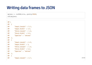
![Reading data from JSON {jsonlite package}Reading data from JSON {jsonlite package}
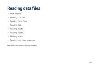
library(jsonlite)
# Using chembl api
jsonData <- fromJSON("https://www.ebi.ac.uk/chemblws/compounds/CHEMBL1.json")
names(jsonData)
## [1] "compound"
jsonData$compound$chemblId
## [1] "CHEMBL1"
jsonData$compound$stdInChiKey
## [1] "GHBOEFUAGSHXPO-XZOTUCIWSA-N"
19/40](https://image.slidesharecdn.com/datahandlinginr-140822100523-phpapp01/85/Data-handling-in-r-19-320.jpg)
![Connecting and listing databasesConnecting and listing databases
library(DBI)
library(RMySQL)
ucscDb <- dbConnect(MySQL(),user="genome",
host="genome-mysql.cse.ucsc.edu")
result <- dbGetQuery(ucscDb,"show databases;"); dbDisconnect(ucscDb);
## [1] TRUE
head(result)
## Database
## 1 information_schema
## 2 ailMel1
## 3 allMis1
## 4 anoCar1
## 5 anoCar2
## 6 anoGam1
25/40](https://image.slidesharecdn.com/datahandlinginr-140822100523-phpapp01/85/Data-handling-in-r-25-320.jpg)
![Connecting to hg19 and listing tablesConnecting to hg19 and listing tables
library(RMySQL)
hg19 <- dbConnect(MySQL(),user="genome", db="hg19",
host="genome-mysql.cse.ucsc.edu")
allTables <- dbListTables(hg19)
length(allTables)
## [1] 11006
allTables[1:5]
## [1] "HInv" "HInvGeneMrna" "acembly" "acemblyClass"
## [5] "acemblyPep"
26/40](https://image.slidesharecdn.com/datahandlinginr-140822100523-phpapp01/85/Data-handling-in-r-26-320.jpg)
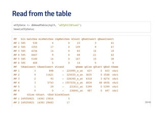
![Get dimensions of a specific tableGet dimensions of a specific table
dbListFields(hg19,"affyU133Plus2")
## [1] "bin" "matches" "misMatches" "repMatches" "nCount"
## [6] "qNumInsert" "qBaseInsert" "tNumInsert" "tBaseInsert" "strand"
## [11] "qName" "qSize" "qStart" "qEnd" "tName"
## [16] "tSize" "tStart" "tEnd" "blockCount" "blockSizes"
## [21] "qStarts" "tStarts"
dbGetQuery(hg19, "select count(*) from affyU133Plus2")
## count(*)
## 1 58463
27/40](https://image.slidesharecdn.com/datahandlinginr-140822100523-phpapp01/85/Data-handling-in-r-27-320.jpg)
![Select a specific subsetSelect a specific subset
query <- dbSendQuery(hg19, "select * from affyU133Plus2 where misMatches between 1 and 3")
affyMis <- fetch(query); quantile(affyMis$misMatches)
## 0% 25% 50% 75% 100%
## 1 1 2 2 3
affyMisSmall <- fetch(query,n=10); dbClearResult(query);
## [1] TRUE
dim(affyMisSmall)
## [1] 10 22
# close connection
dbDisconnect(hg19)
29/40](https://image.slidesharecdn.com/datahandlinginr-140822100523-phpapp01/85/Data-handling-in-r-29-320.jpg)
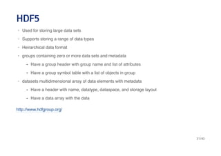
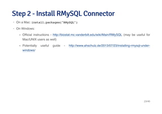
![Creating an HDF5 file and group hierarchyCreating an HDF5 file and group hierarchy
library(rhdf5)
h5createFile("myhdf5.h5")
## [1] TRUE
h5createGroup("myhdf5.h5","foo")
## [1] TRUE
h5createGroup("myhdf5.h5","baa")
## [1] TRUE
h5createGroup("myhdf5.h5","foo/foobaa")
## [1] TRUE
33/40](https://image.slidesharecdn.com/datahandlinginr-140822100523-phpapp01/85/Data-handling-in-r-33-320.jpg)
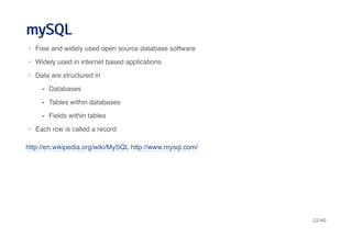
![hdf5 continuedhdf5 continued
Saving multiple objects to an HDF5 file
h5ls("myhdf5.h5")
## group name otype dclass dim
## 0 / baa H5I_GROUP
## 1 / foo H5I_GROUP
## 2 /foo foobaa H5I_GROUP
A = 1:7; B = 1:18; D = seq(0,1,by=0.1)
h5save(A, B, D, file="newfile2.h5")
h5dump("newfile2.h5")
## $A
## [1] 1 2 3 4 5 6 7
##
## $B
## [1] 1 2 3 4 5 6 7 8 9 10 11 12 13 14 15 16 17 18
## 34/40](https://image.slidesharecdn.com/datahandlinginr-140822100523-phpapp01/85/Data-handling-in-r-34-320.jpg)


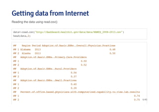
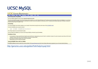
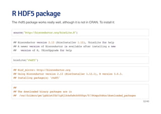
The document provides a comprehensive guide on data handling in R, covering how to set working directories, read various data file formats, and connect to databases like MySQL. It emphasizes tools such as read.csv, jsonlite for JSON, and the rhdf5 package for HDF5 files. Additionally, it includes specific commands for downloading files and accessing data from APIs and databases.