R is a language and environment for statistical computing and graphics. It is based on S, an earlier language developed at Bell Labs. R features include being cross-platform, open source, having a package-based repository, strong graphics capabilities, and active user and developer communities. Useful URLs and books for learning R are provided. Instructions for installing R and RStudio on different platforms are given. R can be used for a wide range of statistical analyses and data visualization.

1. R basics
Sagun Baijal
Monday, October 05, 2015

2. Overview
What is R?
R’s correspondence with S
R features
Useful URLs
Installing R, RStudio
R and Statistics
Using R - Getting Started

3. What is R?
R is a language and environment for Statistical Computing and
Graphics.
It is based on S - a language earlier developed at Bell Labs.
R features:
Cross-platform
Free/Open Source Software
Package-based, rich repository of all sorts of packages
Strong graphic capabilities
Strong user, developer communities, active development
Useful URLs:
http://cran.r-project.org
http://www.r-project.org/doc/bib/R-books.html
http://www.r-bloggers.com
http://cookbook-r.com
http://stats.stackexchange.com/
http://www.statmethods.net/
https://www.rstudio.com/

4. Contd. . .
Useful R books:
R in Action by Robert I. Kabacoff. Pub.: Manning Publications
Statistical Analysis with R by John M. Quick. Pub.: PACKT
Publishing
Many more R e-books available through Books24X7 (available
to CDAC through MCIT consortium).

5. Contd. . .
Installing R:
R can be downloaded from Comprehensive R Archive Network
(CRAN) (URL mentioned in previous slide)
Latest release is 3.2.2.
Release available for GNU/Linux, Windows and Mac.
For GNU/Linux:
Debian, Ubuntu like: Follow instructions given on -
https://cran.r-project.org/bin/linux/debian/,
https://cran.r-project.org/bin/linux/ubuntu/; run
sudo apt-get install r-base r-base-dev
RHEL like: Follow instructions given on -
https://cran.r-project.org/bin/linux/redhat/; run
sudo yum install R
For Windows: Follow instructions given on -
https://cran.r-project.org/bin/windows/base/;
Download exe for base package and RTools.
Installing RStudio: RStudio is IDE for R. Available for
GNU/Linux, Windows and Mac. Can be downloaded from URL
given in previous slide for respective platforms.

6. Contd. . .
R and statistics:
A comprehensive statistical platform providing all sorts of data
analytics techniques.
Strong graphics capabilities to visualize complex data.
Designed to support interactive data analysis and exploration.
Capable of reading data from variety of sources.
Facility to program new statistical methods and packages.
Some disadvantages too. . .
Objects stored in primary memory. May impose performance
bottlenecks in case of large datasets.
No provision of built-in dynamic or 3D graphics. But external
packages like plot3D, scatterplot3D etc. available.
Similarly, no built-in support for web-based processing. Can be
done through third-party packages.
Functionality scattered among packages.

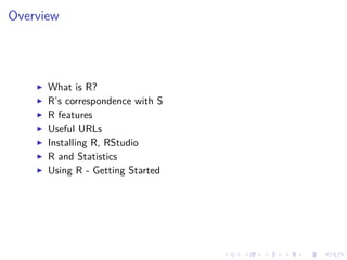
7. Using R - Getting started
Launch R Interface/RStudio depending on your platform.
Utility commands/functions:
setwd() - sets working directory.
setwd("C:/RDemo")
getwd() - gets current working directory.
getwd()
## [1] "C:/RDemo"
dir() - lists the contents of current working directory.
dir()
## [1] "fdata.csv" "Introduction-to-R.ht
## [3] "Introduction-to-R.pdf" "Introduction-to-R.Rm
## [5] "Introduction-to-R_files" "R-basics.html"
## [7] "R-basics.pdf" "R-basics.Rmd"
## [9] "R-introduction-1.pdf" "R-introduction-2.pdf
## [11] "R-introduction-3.pdf" "R-introduction-4.pdf

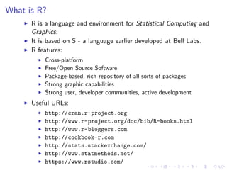
8. Contd. . .
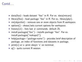
help.start() - provides general help.
help(“foo”) or ?foo - help on function “foo”. For ex.
help(“mean”) or ?mean.
help.search(“foo”) or ??foo - search for string “foo” in help
system. For ex. help.search(“mean”) or ??mean
example(“foo”) - shows examples of function “foo”.
example("mean")
##
## mean> x <- c(0:10, 50)
##
## mean> xm <- mean(x)
##
## mean> c(xm, mean(x, trim = 0.10))
## [1] 8.75 5.50
data() - lists all example datasets in currently loaded packages.
library() - lists all available packages

9. Contd. . .
data(foo) - loads dataset “foo” in R. For ex. data(mtcars)
library(foo) - load package “foo” in R. For ex. library(plyr).
rm(objectlist) - removes one or more objects from R workspace.
options() - shows/sets current options for workspace.
history(#) - lists last # commands. default 25.
install.packages(“foo”) - installs package “foo”. For ex.
install.packages(“reshape2”).
help(package=“package-name”) - provides brief description of
package, an index of functions and datasets in package.
print(x) or x- print obejct ‘x’ on terminal.
q() - quits current R session.

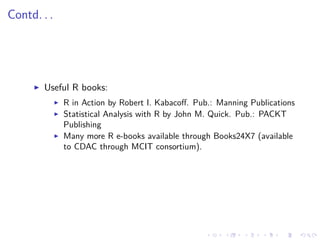
10. Using R - Data types
Five basic types in R are - character, numeric, integer, complex,
logical(true/false).
Common data objects are - vector, matrix, list, factor, data
frame, table.
Creating and assigning to a variable:
x<-1
Checking the type of variable:
class(x)
## [1] "numeric"

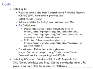
11. Contd. . .
Printing a variable:
x #auto-printing
## [1] 1
print(x) #explicit printing
## [1] 1
Creating Vector: contains objects of same class.
x<-c(1,2,3) #using c() function
y<-vector("logical", length=10) #using vector() function
length(x) #length of vector x
## [1] 3

12. Contd. . .
Vector operations: Various arithmetic operations can be
performed member-wise.
y<-c(4,5,6)
5*x #multiplication by a scalar
## [1] 5 10 15
x+y #addition of two vectors
## [1] 5 7 9
x*y #multiplication of two vectors
## [1] 4 10 18
x^y #x to the power y

13. Contd. . .
Creating Matrix: Two-dimensional array having elements of
same class.
m<-matrix(c(1,2,3,11,12,13), nrow=2,ncol=3) #using matrix()
m
## [,1] [,2] [,3]
## [1,] 1 3 12
## [2,] 2 11 13
dim(m) #dimensions of matrix m
## [1] 2 3
attributes(m) #attributes of matrix m
## $dim
## [1] 2 3

14. Contd. . .
By default, elements in matrix are filled by column. “byrow”
attribute of matrix() can be used to fill elements by row.
m<-matrix(c(1,2,3,11,12,13), nrow=2,ncol=3, byrow = TRUE)
m
## [,1] [,2] [,3]
## [1,] 1 2 3
## [2,] 11 12 13

15. Contd. . .
cbind-ing and rbind-ing: By using cbind() and rbind() functions
x<-c(1,2,3)
y<-c(11,12,13)
cbind(x,y)
## x y
## [1,] 1 11
## [2,] 2 12
## [3,] 3 13
rbind(x,y)
## [,1] [,2] [,3]
## x 1 2 3
## y 11 12 13

16. Contd. . .
Matrix operations/functions:
p<-3*m #multiplication by a scalar
n<-matrix(c(4,5,6,14,15,16), nrow=2,ncol=3)
q<-m+n #addition of two matrices
o<-matrix(c(4,5,6,14,15,16), nrow=3,ncol=2)
r<-m %*% o #matrix multiplication by using %*%
mdash<-t(m) #transpose of matrix
s<-matrix(c(4,5,6,14,15,16,24,25,26), nrow=3,ncol=3,
byrow=TRUE)
s_det<-det(s) #determinant of s
m_row_sum<-rowSums(m)
m_col_sum<-colSums(m)

17. Contd. . .
p
## [,1] [,2] [,3]
## [1,] 3 6 9
## [2,] 33 36 39
q
## [,1] [,2] [,3]
## [1,] 5 8 18
## [2,] 16 26 29
r
## [,1] [,2]
## [1,] 32 92
## [2,] 182 542

18. Contd. . .
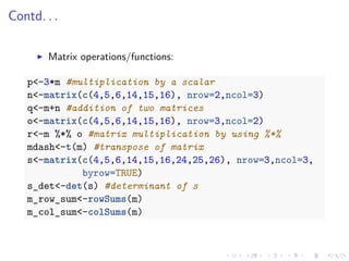
mdash
## [,1] [,2]
## [1,] 1 11
## [2,] 2 12
## [3,] 3 13
s_det
## [1] 1.110223e-14
m_row_sum
## [1] 6 36
m_col_sum
## [1] 12 14 16

19. Contd. . .
List: A special type of vector containing elements of different
classes
x<-list(1,"p",TRUE,2+4i) #using list() function
x
## [[1]]
## [1] 1
##
## [[2]]
## [1] "p"
##
## [[3]]
## [1] TRUE
##
## [[4]]
## [1] 2+4i

20. Contd. . .
Factor: Represents categorical data. Can be ordered or
unordered.
status<-c("low","high","medium","high","low")
x<-factor(status, ordered=TRUE,
levels=c("low","medium","high")) #using factor(
x
## [1] low high medium high low
## Levels: low < medium < high
‘levels’ argument is used to set the order of levels.
First level forms the baseline level.
Without any order, levels are called nominal. Ex. - Type1,
Type2, . . .
With order, levels are called ordinal. Ex. - low, medium, . . .

21. Contd. . .
Data frame: Used to store tabular data. Can contain different
classes
student_id<-c(1,2,3)
student_names<-c("Ram","Shyam","Laxman")
position<-c("First","Second","Third")
data<-data.frame(student_id,student_names,position) #using
data
## student_id student_names position
## 1 1 Ram First
## 2 2 Shyam Second
## 3 3 Laxman Third
data$student_id #accessing a particular column
## [1] 1 2 3

22. Contd. . .
nrow(data) #no. of rows in data
## [1] 3
ncol(data) #no. of columns in data
## [1] 3
names(data) #column names of data
## [1] "student_id" "student_names" "position"

23. Using R - Control structures
R provides all types of control structures: if-else, for, while,
repeat, break, next, return.
Mainly used within functions/scripts.
x<-5
if(x > 7) #if-else structure
y<-TRUE else
y<-FALSE
y
## [1] FALSE
for(i in 1:10) #for loop
print(i)
## [1] 1
## [1] 2
## [1] 3

24. Contd. . .
count<-0
while(count < 10) #while loop
count<-count+1
count
## [1] 10
repeat is used to create an infinite loop. It can be terminated
only through a call to break.
next is used to skip an interation in a loop.
return is used to return a value from a function.

25. Using R - looping functions
These functions can be used loop over various type of objects.
lapply - loop over a list and evaluate a function on each
element.
sapply - same as lapply but try to simplify the result.
apply - apply a function over the margins of an array
tapply - apply a function over the subsets of a vector
x<-list(a=1:5,b=rnorm(20))
lapply(x,sum) #lapply returns a list
## $a
## [1] 15
##
## $b
## [1] -1.487833

26. Contd. . .
x<-matrix(c(1,2,3,11,12,13), nrow=2, ncol=3,byrow=TRUE)
# MARGIN=1 for rows, MARGIN=2 for columns
apply(x,MARGIN=1,FUN=sum)
## [1] 6 36
y<-c(rnorm(20),runif(20),rnorm(20,1))
f<-gl(3,20) #generate factor levels as per given pattern
tapply(y,f,mean)
## 1 2 3
## 0.05429977 0.51238618 0.87080628

27. Using R - Subsetting
Refers to extract sub-segment of data from R objects.
Important while working with large datasets.
There are various operators.
[ used to extract the object of same class as original generally
from a vector or matrix.
[[ used to extract elements of a list or data frame.
$ used to extract elements from a list or data frame by name.
x<-c(1,2,3,4)
x[2]
## [1] 2
x[1:3]
## [1] 1 2 3

28. Contd. . .
Subsetting a matrix:
x<-matrix(c(1,2,3,11,12,13), nrow=2, ncol=3,byrow=TRUE)
x[1,2]
## [1] 2
x[1,]
## [1] 1 2 3
x[,2]
## [1] 2 12

29. Contd. . .
Subsetting a list:
x<-list(a=1,b="p",c=TRUE,d=2+4i)
x[[1]]
## [1] 1
x$d
## [1] 2+4i
x[["c"]]
## [1] TRUE
x["b"]
## $b

30. Contd. . .
Subsetting a data frame
data[1,]
## student_id student_names position
## 1 1 Ram First
data$student_names
## [1] Ram Shyam Laxman
## Levels: Laxman Ram Shyam
data[data$position=="Second",]
## student_id student_names position
## 2 2 Shyam Second
Using logical ANDs and ORs

31. Using R - Functions
Created using the function() directive.
Can be passed as arguments to other functions. Can be nested.
Return value is the last expression to be evaluated inside
function body.
Have named arguments with default values.
Some arguments can be missing during function calls.
add<-function(a=1,b=2,c=3) {
s = a+b+c
print(s)
}
add()
## [1] 6
add(10,11,12)
## [1] 33

32. R Source files
Should be saved/created with .R extension.
Can be used to store functions, commands required to be
executed sequentially etc.
source() function used to load such R scripts into R workspace.
source("C:/RDemo/test.R")
add()
## [1] 6

33. Contd. . .
source("C:/RDemo/test1.R", echo=T)
##
## > x <- 1
##
## > y <- 2
##
## > x + y
## [1] 3
source("C:/RDemo/test1.R", print.eval=T)
## [1] 3

34. References
http://cran.r-project.org
http://www.r-project.org/doc/bib/R-books.html
http://www.r-bloggers.com
http://cookbook-r.com
http://stats.stackexchange.com/
http://www.statmethods.net/
https://www.rstudio.com/
https://github.com/DataScienceSpecialization/
courses/tree/master/02_RProgramming