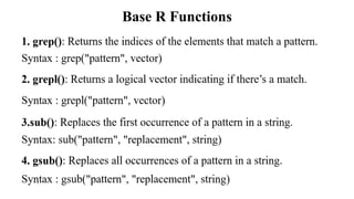
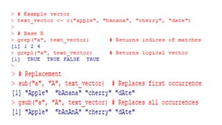
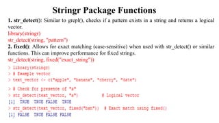
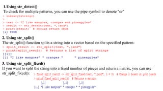
The document provides an overview of data analytics using R, focusing on the handling of datasets and various file types such as CSV, XML, JSON, and Excel. It covers functions for importing and exporting data, manipulating strings, and reshaping data, along with packages for database connectivity and data cleaning. Additionally, it includes examples of using SQL queries and the application of various functions for data processing tasks.

1. Data Analytics With R
Prof.Navyashree K S
Assistant Professor
Dept.of CSE (Data Science)
Sub code: BDS306C
Module 3

2. Datasets
A dataset is a data collection presented in a table.
We can see datasets available in the loaded packages using the data() function.
Most Used built-in Datasets in R
In R, there are tons of datasets we can try but the mostly used built-in datasets
are:
•airquality - New York Air Quality Measurements
•AirPassengers - Monthly Airline Passenger Numbers 1949-1960
•mtcars - Motor Trend Car Road Tests
•iris - Edgar Anderson's Iris Data
https://stat.ethz.ch/R-manual/R-devel/library/datasets/html/00Index.html

3. Display R datasets
Get Information's of Dataset

4. Display Variables Value in R

5. Sort Variables Value in R
Statistical Summary of Data in R
Importing and Exporting Files
1. Text and CSV Files
Reading Data in R
1.Common Formats:
1. CSV, XML, JSON, and YAML are common text formats.
2. CSV (Comma Separated Values) is commonly used for tabular data.

6. Reading CSV Files:
• Use read.table() to read CSV files into a data frame.
• Important arguments:
• header = TRUE: Indicates the presence of a header row.
• fill = TRUE: Allows for unequal rows by filling missing values.
• sep: Specifies the field separator (default is comma).
• nrow: Specifies the number of rows to read.
• skip: Specifies how many lines to skip at the start.
Special Functions:
•read.csv(): Defaults to comma as the separator and assumes a header.
•read.csv2(): Uses semicolon as a separator and comma for decimals.
•read.delim(): Imports tab-delimited files with full stops for decimals.
•read.delim2(): Imports tab-delimited files with commas for decimals.
•Partial Data Reading:
•Packages like colbycol and sqldf allow reading specific rows/columns.
•scan(): Provides low-level control for importing CSV files.
•Handling Missing Values:
•Use na.strings to specify how to treat missing values (e.g., na.strings = "NULL" for SQL).

7. Writing Data in R
1.Writing Data:
•Use write.table() and write.csv() to export data frames to files.
•Key arguments:
•row.names = FALSE: Excludes row names in the output file.
•fileEncoding: Specifies character encoding.
Example: write.csv(deer_data, "F:/deer.csv", row.names = FALSE, fileEncoding = "utf8")
File Location and Structure
1.Locating Files:
•Use the file() function to locate files within a package (e.g., system.file()).
2.Understanding Data Structure:
•Use str() to display the structure of a data frame, showing variable types and observations.
3.Installation and Library Usage:
•Install packages using install.packages(), and load them with library().

8. Example Workflow
1. Install and load a package:

9. 2. Load a dataset from a package:
3.Check the structure of the loaded data:

10. Unstructured Files
Reading and Writing Unstructured Files in R
1.Reading Unstructured Text Files:
•Use readLines() to read files as lines of text.
•Accepts the file path as an argument.
•Returns a character vector where each element represents a line in the file
> tempest <- readLines("F:/deer.csv")
> print(tempest)

11. 2.Writing to Unstructured Text Files:
•Use writeLines() to write text or a character vector to a file.
•Takes the text to be written and the file path as arguments.
> writeLines("This book is about a story by Shakespeare", "F:/story.csv")
Key Functions
•readLines():
•Purpose: Reads a text file line by line.
•Argument: Path to the file.
•writeLines():
•Purpose: Writes a string or character vector to a specified file.
•Arguments: Text content and the desired file path.
XML and HTML Files
1.XML Files:
1. Used for storing nested data structures (e.g., RSS feeds, SOAP
protocols, XHTML web pages).
2. Requires the XML package for reading.

12. •Reading XML Files:
•Use the xmlParse() function to import XML files.
•Arguments:
•useInternalNodes = FALSE: If set to FALSE, uses R-level nodes instead of internal nodes
(default behavior is set by xmlTreeParse()).
•Node Querying:
•When using internal nodes, you can query the node tree using XPath, which is a language
designed for interrogating XML documents.
Example Workflow
1.Install and Load the XML Package:
install.packages("XML")
library(XML)
2.Importing an XML File:
xml_file <- system.file("extdata", "options.xml", package = "learningr")
r_options <- xmlParse(xml_file) # Using internal nodes
Use system.file() to locate the XML file within a package.
Use xmlParse() to read the XML file

13. Options for Parsing:
•To use R-level nodes instead of internal nodes:
xmlParse(xml_file, useInternalNodes = FALSE)
•For a tree structure:
xmlTreeParse(xml_file)
Working with HTML Files
1.Functions for HTML:
•Use htmlParse() to import HTML files.
•Use htmlTreeParse() for a tree structure, similar to xmlParse() and xmlTreeParse().
html_file <- "path/to/your/file.html"
html_data <- htmlParse(html_file) # Parse HTML

14. JASON and YAML Files
JSON Handling in R
• Best Package: RJSONIO (better performance than rjson)
• Import Function: fromJSON()
• Export Function: toJSON()
install.packages("rjson")
library("rjson")

15. YAML Handling in R
• Package: yaml
• Import Functions:
• yaml.load()
• yaml.load_file()
• Export Function: as.yaml()
Binary Formats
•Advantages: Smaller size, better performance
•Disadvantages: Less human-readable, harder to debug. This format keeps it
straightforward and easy to reference.

16. Excel Files
Excel Formats
•Document Formats: XLS and XLSX
Importing Excel Files
•Functions:
•read.xlsx()
•read.xlsx2()
•Optional Argument: colClasses (determines column classes in the resulting data frame)
Exporting Excel Files
•Function: write.xlsx2()
•Arguments: Data frame and file name
Alternative Package
•Package: xlsReadWrite
•Compatibility: Works only on 32-bit R installations and Windows

17. ➢install.packages("xlsx")
➢library(xlsx)
➢logfile <- read.xlsx2("F:/Log2015.xls", sheetIndex = 1, startRow = 2, endRow = 72,colIndex
= 1:5, colClasses = c("character", "numeric", "character", "character", "integer"))
•File Path: "F:/Log2015.xls" (location of the Excel file)
•sheetIndex: 1 (reads from the first sheet)
•startRow: 2 (starts reading from the second row)
•endRow: 72 (reads up to the 72nd row)
•colIndex: 1:5 (selects columns 1 to 5)
•colClasses: Defines the data types for the columns:
•Column 1: character
•Column 2: numeric
•Column 3: character
•Column 4: character
•Column 5: integer

18. SAS, SPSS, and MATLAB Files
Importing Data
•Package: foreign
•SAS Datasets:
•Function: read.ssd()
•Stata DTA Files:
•Function: read.dta()
•SPSS Files:
•Function: read.spss()
Exporting Data
•Function: write.foreign()
•Allows exporting datasets to SAS, Stata, or SPSS formats.
MATLAB Files
•Package: R.matlab
•Read MATLAB Binary Files:
•Function: readMat()
•Write MATLAB Binary Files:
•Function: writeMat()
Image Files
•Packages for Reading Images:
•jpeg
•png
•tiff
•rtiff
•readbitmap

19. 1. Importing Web Data in R
APIs and Packages
•WDI Package: Accesses World Bank data.
•SmarterPoland Package: Accesses Polish government data.
•twitter Package: Provides access to Twitter users and their tweets.
2.Importing Data from URLs
•Function: read.table().Can accept a URL as an argument, allowing direct reading of data from
the web.
3. Downloading Data
•Function: download.file()
•Recommended for large files or frequently accessed data.
•Creates a local copy for faster access and easier import.
WEB DATABASE

20. Accessing Databases
• To access SQLite databases in R using the DBI package and RSQLite, you
can follow these steps:
1. Install the necessary packages (if you haven't already):
install.packages("DBI")
install.packages("RSQLite")
2.Load the packages
library(DBI)
library(RSQLite)
3.Define a database driver for SQLite:
# Define the SQLite driver
sqlite_driver <- dbDriver("SQLite")

21. 4.Set up a connection to the database
# Create a connection to the SQLite database
# Replace 'your_database.sqlite' with the path to your database file
con <- dbConnect(sqlite_driver, dbname = "your_database.sqlite")
5. Retrieve data using a SQL query:
# Write your SQL query as a string
query <- "SELECT * FROM your_table_name" # Replace with your actual SQL query
# Send the query to the database and retrieve the data
data <- dbGetQuery(con, query)
6. Close the connection when done
dbDisconnect(con)

22. Using dbReadTable() and dbListTables()
1.Reading a Table:
•You can use dbReadTable() to read a complete table from a connected database.
data <- dbReadTable(con, "idblock")
print(data)
2. Listing All Tables:
•Use dbListTables() to get a list of all tables in the connected database.
tables <- dbListTables(con)
print(tables)
3. Disconnecting and Unloading the Driver
•Disconnecting from the Database:
•Use dbDisconnect() to close the connection to the database.
4. Unloading the Driver:
•Use dbUnloadDriver() to unload the database driver when it's no longer needed.

23. Database Packages
1.DBI:A general interface for database access in R. Provides a unified set of functions to work with
various database systems.(dbconnect(), dbDisconnect(), dbListTables())
2.RSQLite:A package that allows R to connect to SQLite databases. lightweight and file-based,It
provides functions to create, read, and manage SQLite databases.
3.RMySQL:A package used to connect to MySQL databases. It facilitates running queries and retrieving
results. It’s suited for larger, multi-user environments.
4.RPostgreSQL:Enables connections to PostgreSQL databases. Similar functionality as RMySQL but
tailored for PostgreSQL's features like JSON data types, window functions, and full-text search. It's
designed for robust data handling and complex queries.
5.ROracle:Used to connect to Oracle databases, providing access to Oracle's specific SQL features
Inncluding PL/SQL procedures, which allow for complex database operations.
6.RODBC:A package for connecting to databases using ODBC (Open Database Connectivity). It's
versatile and allows connections to various databases like SQL Server and Access.
7.RMongo and rmongodb:Packages designed for connecting to MongoDB, a popular NoSQL database.
They provide functions to interact with MongoDB collections.
8.RCassandra:A package for accessing Cassandra, another NoSQL database. It allows for managing and
querying Cassandra databases.

24. Data Cleaning and Transforming
1. Manipulating Strings
In some datasets or data frames logical values are represented as “Y” and “N” instead of
TRUE and FALSE. In such cases it is possible to replace the string with correct logical value
as in the example below

25. Base R Functions

27. Stringr Package Functions
1. str_detect(): Similar to grepl(), checks if a pattern exists in a string and returns a logical
vector.
library(stringr)
str_detect(string, "pattern")
2. fixed(): Allows for exact matching (case-sensitive) when used with str_detect() or similar
functions. This can improve performance for fixed strings.
str_detect(string, fixed("exact_string"))

28. 1.Using str_detect()
To check for multiple patterns, you can use the pipe symbol to denote "or"
2. Using str_split()
The str_split() function splits a string into a vector based on the specified pattern:
3. Using str_split_fixed()
If you want to split the string into a fixed number of pieces and return a matrix, you can use
str_split_fixed():

29. 4. Counting multiple patterns: You can use the pipe symbol (|) to count occurrences of
either pattern.
5. Counting a single pattern: You can also count occurrences of a single character or substring.
6. str_replace(): Replaces only the first occurrence of a specified pattern in the text.

30. 7.str_replace_all(): Replaces all occurrences of a specified pattern in the text.
Replacing multiple patterns: You can specify characters to replace by using square brackets.
For example, to replace all occurrences of "a" or "o":

31. Manipulating Data Frames
Two ways to add a column to a data frame in R by calculating the period between the
start_date and end_date. Both methods effectively achieve the same result.

33. The within() function allows you to add multiple columns to a data frame in a more concise
way than with(). Here's how you can use the within() function and also the mutate()
function from the dplyr package to achieve the same result. Ex: Using Within()

34. Using mutate() from dplyr package

35. Handling Missing Values
1. complete.cases(): Returns the rows without any missing values.
2. na.omit(): Removes rows with missing values.

36. 3.na.fail(): Throws an error if there are any missing values.

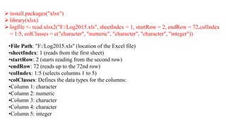
37. Selecting Columns and Rows
1.Selecting Specific Columns, Selecting Specific Rows:
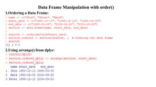
Sorting and Ordering
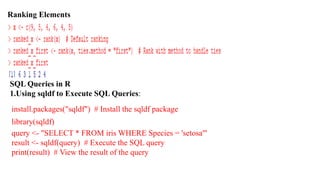
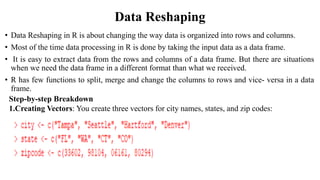
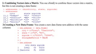
1.Sorting Vectors:
2.Using order():
x <- c(5, 2, 8, 1, 4)
order_indices <- order(x)
sorted_x <- x[order_indices]
print(sorted_x) # Output: 1 2 4 5 8

38. Data Frame Manipulation with order()
1.Ordering a Data Frame:
2.Using arrange() from dplyr:

39. Ranking Elements
SQL Queries in R
1.Using sqldf to Execute SQL Queries:
install.packages("sqldf") # Install the sqldf package
library(sqldf)
query <- "SELECT * FROM iris WHERE Species = 'setosa'"
result <- sqldf(query) # Execute the SQL query
print(result) # View the result of the query

40. Data Reshaping
• Data Reshaping in R is about changing the way data is organized into rows and columns.
• Most of the time data processing in R is done by taking the input data as a data frame.
• It is easy to extract data from the rows and columns of a data frame. But there are situations
when we need the data frame in a different format than what we received.
• R has few functions to split, merge and change the columns to rows and vice- versa in a data
frame.
Step-by-step Breakdown
1.Creating Vectors: You create three vectors for city names, states, and zip codes:

41. 2. Combining Vectors into a Matrix: You use cbind() to combine these vectors into a matrix,
but this is not creating a data frame:
3.Creating a New Data Frame: You create a new data frame new.address with the same
columns

42. 4. Combining Data Frames with rbind(): You use rbind() to combine the original addresses
with the new addresses:
The merge() function in R to combine two datasets based on the columns
1. Load the Necessary Library: Make sure you have the package loaded to access the
datasets.

43. 2. Inspect the Datasets: Check the structure and contents of datasets.
•Merging Keys: The merge is done on the ID
column, which is present in both data frames.
•Non-Matched Rows: ID 1 from Data Frame A and
ID 4 from Data Frame B do not match, so they are
excluded from the result.
3. Merging the Datasets: Use the merge() function to combine the two datasets based on
the specified columns.

44. 4. Inspect the Merged Data: Check the first few rows of the merged dataset and the
number of rows in the merged result.

45. The reshape2 package provides handy functions like melt() and cast() to facilitate this
process. Let's break down the steps you've described using the ships dataset from the MASS
library.
1. Loading the Necessary Libraries and Data
2. Melting the Data
Next, we use the melt() function to transform
the dataset from wide to long format. This is
useful when we want to organize the data by
keeping certain identifiers (in this case, type
and year) while converting other columns into
key-value pairs.

46. 3. Checking the Number of Rows
4. Casting the Data

47. Grouping Functions
1. apply()
•Purpose: Apply a function over the margins of an array or matrix.
•Usage: apply(X, MARGIN, FUNCTION)
•MARGIN = 1 for rows, 2 for columns.
2. lapply()
•Purpose: Apply a function to
each element of a list or vector
and return a list.
•Usage: lapply(X, FUNCTION)

48. 3. sapply()
•Purpose: Similar to lapply(), but attempts to simplify the result to a vector or
matrix when possible.
•Usage: sapply(X, FUNCTION)

49. 4.vapply()
•Purpose: Like sapply(), but requires you to specify the type and length of the output, leading to
potentially better performance.
•Usage: vapply(X, FUN, FUN.VALUE)

50. 5. mapply()
•Purpose: A multivariate version of sapply(), allowing you to apply a function to multiple
arguments.
•Usage: mapply(FUN, MoreArgs = NULL)
6. tapply()
•Purpose: Apply a function over subsets of a vector, defined by a factor or factors.
•Usage: tapply(X, INDEX, FUNCTION)

51. 7.by()
•Purpose: Apply a function to a data frame or matrix split by one or more factors.
•Usage: by(data, INDICES, FUN)
8. rapply()
•Purpose: Recursively apply a function to all elements of a nested list.
•Usage: rapply(X, f, how = "replace", classes = "list")
Performance Considerations
•Use vapply() when you know the output type and want to maximize performance.
•Choose sapply() when you prefer simpler output without caring much about performance.
•Use lapply() when you want a list as the output, regardless of its simplicity.
These functions significantly enhance R's ability to handle data efficiently, enabling users to perform
complex operations with minimal code.

52. 9. aggregate(x, by, FUNCTION)
In R, the aggregate() function is used to compute summary statistics of a data frame or
matrix, grouped by one or more factors. It allows you to easily summarize data and can be
very useful for exploratory data analysis.
Parameters
•x: A data frame or a matrix containing the data you want to aggregate.
•by: A list of factors or grouping variables that define how to aggregate the data.
•FUN: The function to be applied to each group (e.g., mean, sum, length, etc.).