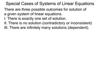
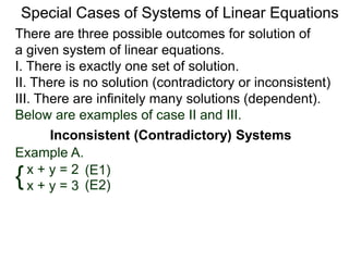
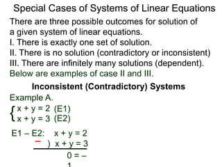
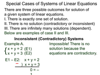
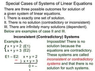
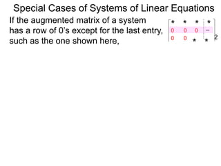
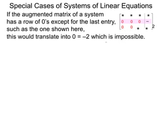
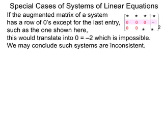
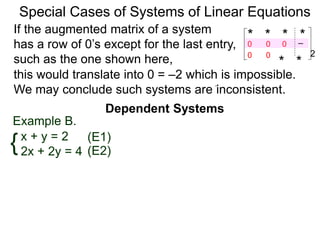
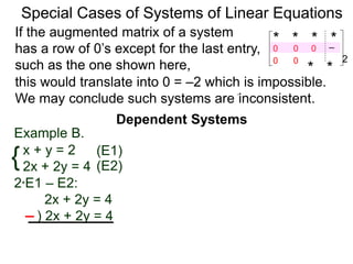
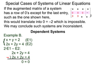
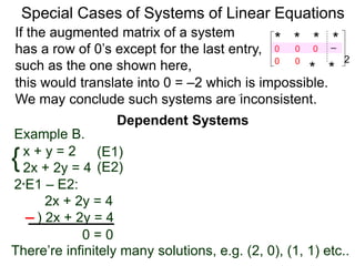
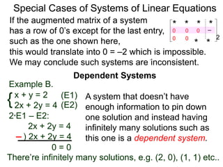
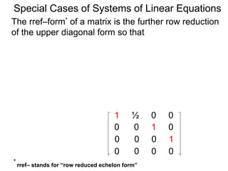
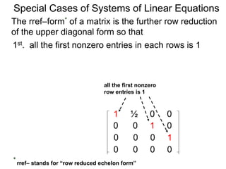
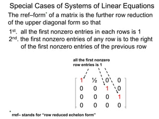
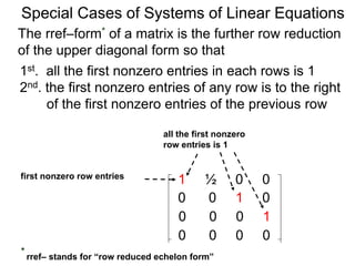
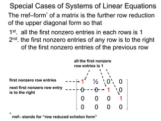
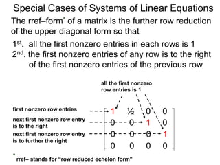
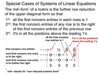
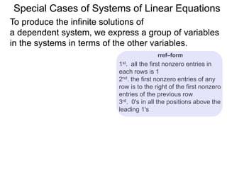
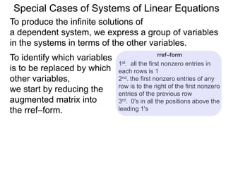
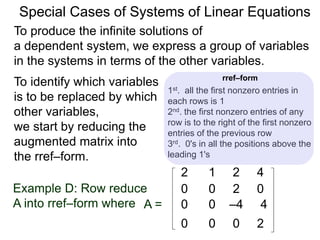
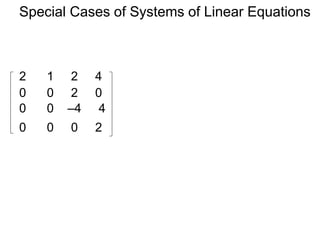
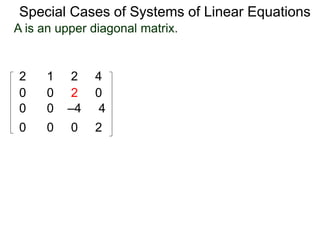
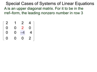
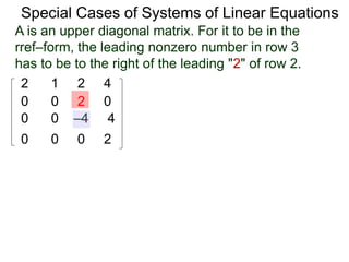
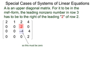
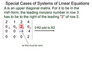
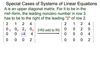
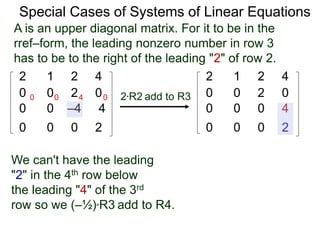
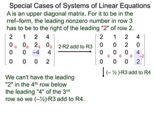
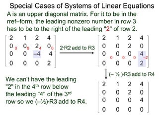
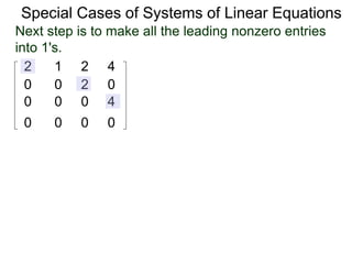
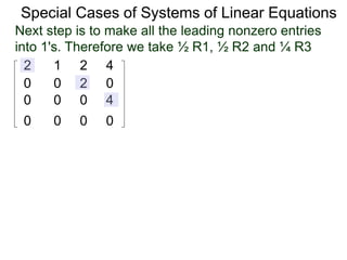
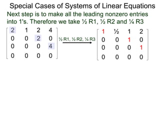
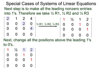
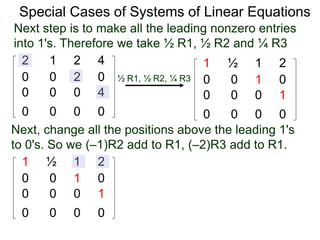
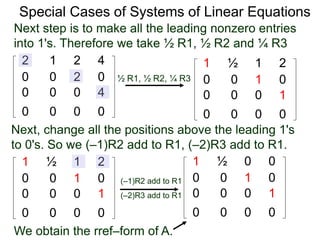
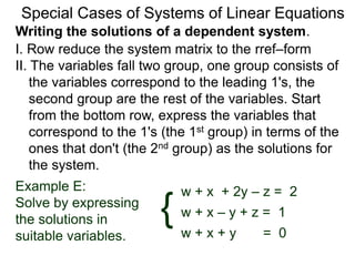
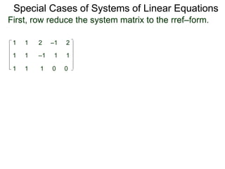
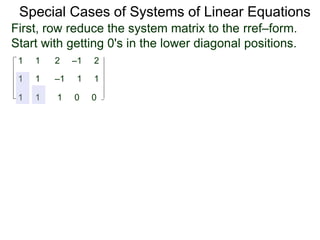
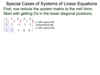
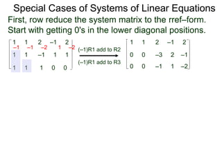
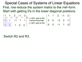
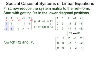
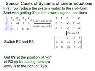
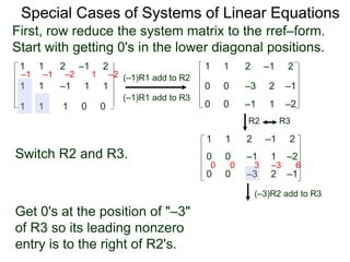
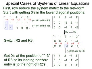
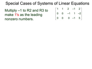
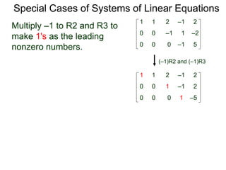
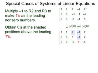
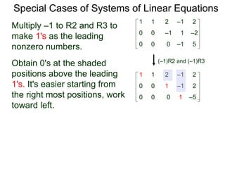
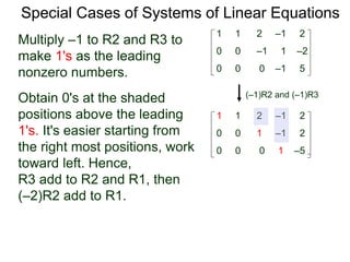
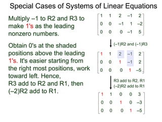
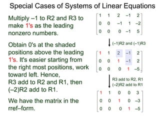
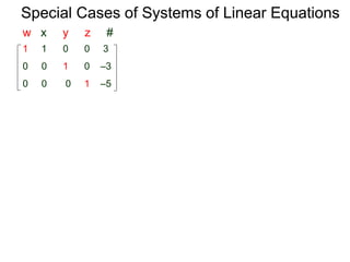
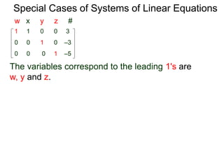
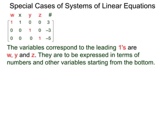
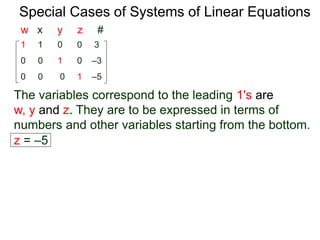
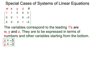
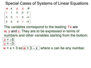
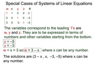
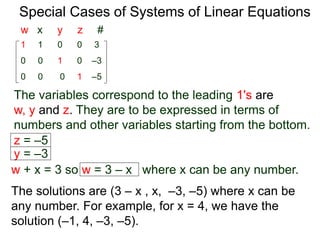
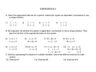
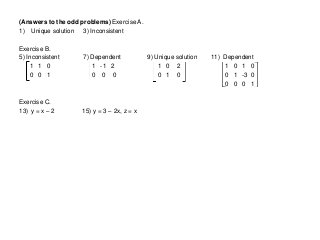
Special Cases of Systems of Linear Equations
There are three possible outcomes for the solution of
a given system of linear equations.
Special Cases of Systems of Linear Equations
There are three possible outcomes for the solution of
a given system of linear equations.
I. There is exactly one solution.
II. There is no solution (contradictory or inconsistent)
III. There are infinitely many solutions (dependent).
Special Cases of Systems of Linear Equations
There are three possible outcomes for the solution of
a given system of linear equations.
I. There is exactly one solution.
II. There is no solution (contradictory or inconsistent)
III. There are infinitely many solutions (dependent).
Special Cases of Systems of Linear Equations
Below are examples of case II and III.
There are three possible outcomes for the solution of
a given system of linear equations.
I. There is exactly one solution.
II. There is no solution (contradictory or inconsistent)
III. There are infinitely many solutions (dependent).
Special Cases of Systems of Linear Equations
Inconsistent (Contradictory) Systems
{x + y = 2
x + y = 3
(E1)
(E2)
Example A.
Below are examples of case II and III.
There are three possible outcomes for the solution of
a given system of linear equations.
I. There is exactly one solution.
II. There is no solution (contradictory or inconsistent)
III. There are infinitely many solutions (dependent).
Special Cases of Systems of Linear Equations
Inconsistent (Contradictory) Systems
{x + y = 2
x + y = 3
E1 – E2: x + y = 2
) x + y = 3
0 = –1
Impossible! There is no
solution because the
equations are contradictory.
These systems are called
inconsistent or contradictory
systems and that there is no
solution for such systems.
(E1)
(E2)
Example A.
Below are examples of case II and III.
Special Cases of Systems of Linear Equations
If the augmented matrix of a system
has a row of 0’s except for the last entry,
such as the one shown here,
* * * *
–2
* *
0
0 0
0 0
Special Cases of Systems of Linear Equations
If the augmented matrix of a system
has a row of 0’s except for the last entry,
such as the one shown here,
* * * *–2
* *
0
0 0
0 0
this would translate into 0 = –2 which is impossible.
Special Cases of Systems of Linear Equations
If the augmented matrix of a system
has a row of 0’s except for the last entry,
such as the one shown here,
* * * *–2
* *
0
0 0
0 0
this would translate into 0 = –2 which is impossible.
We may conclude such systems are inconsistent.
Dependent Systems
Special Cases of Systems of Linear Equations
Example B.
{x + y = 2
2x + 2y = 4
(E1)
(E2)
If the augmented matrix of a system
has a row of 0’s except for the last entry,
such as the one shown here,
* * * *–2
* *
0
0 0
0 0
this would translate into 0 = –2 which is impossible.
We may conclude such systems are inconsistent.
Dependent Systems
Special Cases of Systems of Linear Equations
Example B.
{x + y = 2
2x + 2y = 4
2*E1 – E2:
2x + 2y = 4
) 2x + 2y = 4
0 = 0
(E1)
(E2)
If the augmented matrix of a system
has a row of 0’s except for the last entry,
such as the one shown here,
* * * *–2
* *
0
0 0
0 0
this would translate into 0 = –2 which is impossible.
We may conclude such systems are inconsistent.
There’re infinitely many solutions, e.g. (2, 0), (1, 1) etc..
Dependent Systems
Special Cases of Systems of Linear Equations
Example B.
{x + y = 2
2x + 2y = 4
2*E1 – E2:
2x + 2y = 4
) 2x + 2y = 4
0 = 0
(E1)
(E2)
If the augmented matrix of a system
has a row of 0’s except for the last entry,
such as the one shown here,
* * * *–2
* *
0
0 0
0 0
A system that doesn’t have
enough information to pin down
one solution and instead having
infinitely many solutions such as
this one is a dependent system.
this would translate into 0 = –2 which is impossible.
We may conclude such systems are inconsistent.
There’re infinitely many solutions, e.g. (2, 0), (1, 1) etc..
Special Cases of Systems of Linear Equations
The rref–form* of a matrix is the further row reduction
of the upper diagonal form so that
1 ½ 0 0
0 0 1 0
0 0 0 1
0 0 0 0
* rref– stands for “row reduced echelon form”
Special Cases of Systems of Linear Equations
The rref–form* of a matrix is the further row reduction
of the upper diagonal form so that
1st. all the first nonzero entries in each row are 1
1 ½ 0 0
0 0 1 0
0 0 0 1
0 0 0 0
all the first nonzero
row entries are 1
* rref– stands for “row reduced echelon form”
Special Cases of Systems of Linear Equations
The rref–form* of a matrix is the further row reduction
of the upper diagonal form so that
1st. all the first nonzero entries in each row are 1
2nd. the first nonzero entry of any row is to the right
of the first nonzero entry of the previous row
1 ½ 0 0
0 0 1 0
0 0 0 1
0 0 0 0
first nonzero row entry
next first nonzero row entry
is to the right
next first nonzero row entry
is further to the right
all the first nonzero
row entries are 1
* rref– stands for “row reduced echelon form”
Special Cases of Systems of Linear Equations
The rref–form* of a matrix is the further row reduction
of the upper diagonal form so that
1st. all the first nonzero entries in each row are 1
2nd. the first nonzero entry of any row is to the right
of the first nonzero entry of the previous row
3rd. 0's in all the positions above the leading 1's
0's in all the positions
above the leading 1's.
1 ½ 0 0
0 0 1 0
0 0 0 1
0 0 0 0
first nonzero row entry
next first nonzero row entry
is to the right
next first nonzero row entry
is further to the right
all the first nonzero
row entries are 1
* rref– stands for “row reduced echelon form”
Special Cases of Systems of Linear Equations
To produce the infinite solutions of
a dependent system, we express a group of variables
in the systems in terms of the other variables.
1st. all the first nonzero entries in
each row are 1
2nd. the first nonzero entry of any row
is to the right of the first nonzero
entry of the previous row
3rd. 0's in all the positions above the
leading 1's
rref–form
Special Cases of Systems of Linear Equations
To produce the infinite solutions of
a dependent system, we express a group of variables
in the systems in terms of the other variables.
To identify which variables
are to be replaced by
which other variables,
we start by reducing the
augmented matrix into
the rref–form.
1st. all the first nonzero entries in
each row are 1
2nd. the first nonzero entry of any row
is to the right of the first nonzero
entry of the previous row
3rd. 0's in all the positions above the
leading 1's
rref–form
Special Cases of Systems of Linear Equations
To produce the infinite solutions of
a dependent system, we express a group of variables
in the systems in terms of the other variables.
2 1 2 4
Example D: Row reduce
A into rref–form where A =
0 0 2 0
0 0 –4 4
0 0 0 2
To identify which variables
are to be replaced by
which other variables,
we start by reducing the
augmented matrix into
the rref–form.
1st. all the first nonzero entries in
each row are 1
2nd. the first nonzero entry of any row
is to the right of the first nonzero
entry of the previous row
3rd. 0's in all the positions above the
leading 1's
rref–form
Special Cases of Systems of Linear Equations
2 1 2 4
0 0 2 0
0 0 –4 4
0 0 0 2
Special Cases of Systems of Linear Equations
2 1 2 4
0 0 2 0
0 0 –4 4
0 0 0 2
A is an upper diagonal matrix.
Special Cases of Systems of Linear Equations
2 1 2 4
0 0 2 0
0 0 –4 4
0 0 0 2
A is an upper diagonal matrix.A is an upper diagonal matrix. For it to be in the
rref–form, the leading nonzero number in row 3
Special Cases of Systems of Linear Equations
2 1 2 4
0 0 2 0
0 0 –4 4
0 0 0 2
A is an upper diagonal matrix.A is an upper diagonal matrix. For it to be in the
rref–form, the leading nonzero number in row 3
has to be to the right of the leading "2" of row 2.
Special Cases of Systems of Linear Equations
2 1 2 4
0 0 2 0
0 0 –4 4
0 0 0 2
A is an upper diagonal matrix.A is an upper diagonal matrix. For it to be in the
rref–form, the leading nonzero number in row 3
has to be to the right of the leading "2" of row 2.
so this must be zero
Special Cases of Systems of Linear Equations
2 1 2 4
0 0 2 0
0 0 –4 4
0 0 0 2
2*R2 add to R30 0 4 0
A is an upper diagonal matrix. For it to be in the
rref–form, the leading nonzero number in row 3
has to be to the right of the leading "2" of row 2.
so this must be zero
Special Cases of Systems of Linear Equations
2 1 2 4
0 0 2 0
0 0 –4 4
0 0 0 2
2*R2 add to R3
2 1 2 4
0 0 2 0
0 0 0 4
0 0 0 2
0 0 4 0
A is an upper diagonal matrix. For it to be in the
rref–form, the leading nonzero number in row 3
has to be to the right of the leading "2" of row 2.
Special Cases of Systems of Linear Equations
2 1 2 4
0 0 2 0
0 0 –4 4
0 0 0 2
2*R2 add to R3
2 1 2 4
0 0 2 0
0 0 0 4
0 0 0 2
0 0 4 0
A is an upper diagonal matrix. For it to be in the
rref–form, the leading nonzero number in row 3
has to be to the right of the leading "2" of row 2.
We can't have the leading
"2" in the 4th row below
the leading "4" of the 3rd
row so we (–½)*R3 add to R4.
Special Cases of Systems of Linear Equations
2 1 2 4
0 0 2 0
0 0 –4 4
0 0 0 2
2*R2 add to R3
2 1 2 4
0 0 2 0
0 0 0 4
0 0 0 2
0 0 4 0
We can't have the leading
"2" in the 4th row below
the leading "4" of the 3rd
row so we (–½)*R3 add to R4.
(– ½ )*R3 add to R4
A is an upper diagonal matrix. For it to be in the
rref–form, the leading nonzero number in row 3
has to be to the right of the leading "2" of row 2.
0 0 0 –2
Special Cases of Systems of Linear Equations
2 1 2 4
0 0 2 0
0 0 –4 4
0 0 0 2
2*R2 add to R3
2 1 2 4
0 0 2 0
0 0 0 4
0 0 0 2
0 0 4 0
We can't have the leading
"2" in the 4th row below
the leading "4" of the 3rd
row so we (–½)*R3 add to R4.
(– ½ )*R3 add to R4
2 1 2 4
0 0 2 0
0 0 0 4
0 0 0 0
A is an upper diagonal matrix. For it to be in the
rref–form, the leading nonzero number in row 3
has to be to the right of the leading "2" of row 2.
0 0 0 –2
Special Cases of Systems of Linear Equations
2 1 2 4
0 0 2 0
0 0 0 4
0 0 0 0
Next step is to make all the leading nonzero entries
into 1's.
Special Cases of Systems of Linear Equations
2 1 2 4
0 0 2 0
0 0 0 4
0 0 0 0
Next step is to make all the leading nonzero entries
into 1's. Therefore we take ½ R1, ½ R2 and ¼ R3
Special Cases of Systems of Linear Equations
2 1 2 4
0 0 2 0
0 0 0 4
0 0 0 0
Next step is to make all the leading nonzero entries
into 1's. Therefore we take ½ R1, ½ R2 and ¼ R3
1 ½ 1 2
0 0 1 0
0 0 0 1
0 0 0 0
½ R1, ½ R2, ¼ R3
Special Cases of Systems of Linear Equations
2 1 2 4
0 0 2 0
0 0 0 4
0 0 0 0
Next step is to make all the leading nonzero entries
into 1's. Therefore we take ½ R1, ½ R2 and ¼ R3
1 ½ 1 2
0 0 1 0
0 0 0 1
0 0 0 0
½ R1, ½ R2, ¼ R3
Next, change all the positions above the leading 1's
to 0's.
1 ½ 1 2
0 0 1 0
0 0 0 1
0 0 0 0
Special Cases of Systems of Linear Equations
2 1 2 4
0 0 2 0
0 0 0 4
0 0 0 0
Next step is to make all the leading nonzero entries
into 1's. Therefore we take ½ R1, ½ R2 and ¼ R3
1 ½ 1 2
0 0 1 0
0 0 0 1
0 0 0 0
½ R1, ½ R2, ¼ R3
Next, change all the positions above the leading 1's
to 0's. So we (–1)R2 add to R1, (–2)R3 add to R1.
1 ½ 1 2
0 0 1 0
0 0 0 1
0 0 0 0
(–1)R2 add to R1
(–2)R3 add to R1
1 ½ 0 0
0 0 1 0
0 0 0 1
0 0 0 0
We obtain the rref–form of A.
Writing the solutions of a dependent system.
Special Cases of Systems of Linear Equations
Writing the solutions of a dependent system.
Special Cases of Systems of Linear Equations
I. Row reduce the system matrix to the rref–form
Writing the solutions of a dependent system.
Special Cases of Systems of Linear Equations
I. Row reduce the system matrix to the rref–form
II. The variables falls into two groups, one group
consists of the variables corresponding to the
leading 1's, the second group is the rest of the
variables.
Writing the solutions of a dependent system.
Special Cases of Systems of Linear Equations
I. Row reduce the system matrix to the rref–form
II. The variables falls into two groups, one group
consists of the variables corresponding to the
leading 1's, the second group is the rest of the
variables. Start from the bottom row, express the
variables that correspond to the 1's (the 1st group)
in terms of the ones that don't (the 2nd group) as
the solutions for the system.
w + x + 2y – z = 2Example E:
Solve by expressing
the solutions in
suitable variables.
w + x – y + z = 1
w + x + y = 0
{
1 1 2 –1 2
First, row reduce the system matrix to the rref–form.
1 1 –1 1 1
1 1 1 0 0
Special Cases of Systems of Linear Equations
1 1 2 –1 2
First, row reduce the system matrix to the rref–form.
Start with getting 0's in the lower diagonal positions.
1 1 –1 1 1
1 1 1 0 0
Special Cases of Systems of Linear Equations
1 1 2 –1 2
First, row reduce the system matrix to the rref–form.
Start with getting 0's in the lower diagonal positions.
1 1 –1 1 1
1 1 1 0 0
Special Cases of Systems of Linear Equations
(–1)R1 add to R2
(–1)R1 add to R3
–1 –1 –2 1 –2
1 1 2 –1 2
First, row reduce the system matrix to the rref–form.
Start with getting 0's in the lower diagonal positions.
1 1 –1 1 1
1 1 1 0 0
Special Cases of Systems of Linear Equations
(–1)R1 add to R2
(–1)R1 add to R3
–1 –1 –2 1 –2
1 1 2 –1 2
0 0 –3 2 –1
0 0 –1 1 –2
1 1 2 –1 2
First, row reduce the system matrix to the rref–form.
Start with getting 0's in the lower diagonal positions.
1 1 –1 1 1
1 1 1 0 0
Special Cases of Systems of Linear Equations
(–1)R1 add to R2
(–1)R1 add to R3
–1 –1 –2 1 –2
1 1 2 –1 2
0 0 –3 2 –1
0 0 –1 1 –2
Switch R2 and R3.
1 1 2 –1 2
First, row reduce the system matrix to the rref–form.
Start with getting 0's in the lower diagonal positions.
1 1 –1 1 1
1 1 1 0 0
Special Cases of Systems of Linear Equations
(–1)R1 add to R2
(–1)R1 add to R3
–1 –1 –2 1 –2
1 1 2 –1 2
0 0 –3 2 –1
0 0 –1 1 –2
Switch R2 and R3.
1 1 2 –1 2
0 0 –3 2 –1
0 0 –1 1 –2
R2 R3
1 1 2 –1 2
First, row reduce the system matrix to the rref–form.
Start with getting 0's in the lower diagonal positions.
1 1 –1 1 1
1 1 1 0 0
Special Cases of Systems of Linear Equations
(–1)R1 add to R2
(–1)R1 add to R3
–1 –1 –2 1 –2
1 1 2 –1 2
0 0 –3 2 –1
0 0 –1 1 –2
Switch R2 and R3.
1 1 2 –1 2
0 0 –3 2 –1
0 0 –1 1 –2
R2 R3
Get 0's at the position of "–3"
of R3 so its leading nonzero
entry is to the right of R2's.
1 1 2 –1 2
First, row reduce the system matrix to the rref–form.
Start with getting 0's in the lower diagonal positions.
1 1 –1 1 1
1 1 1 0 0
Special Cases of Systems of Linear Equations
(–1)R1 add to R2
(–1)R1 add to R3
–1 –1 –2 1 –2
1 1 2 –1 2
0 0 –3 2 –1
0 0 –1 1 –2
Switch R2 and R3.
1 1 2 –1 2
0 0 –3 2 –1
0 0 –1 1 –2
(–3)R2 add to R3
0 0 3 –3 6
R2 R3
Get 0's at the position of "–3"
of R3 so its leading nonzero
entry is to the right of R2's.
1 1 2 –1 2
0 0 0 –1 5
0 0 –1 1 –2
Special Cases of Systems of Linear Equations
Multiply –1 to R2 and R3 to
make 1's as the leading
nonzero numbers.
1 1 2 –1 2
0 0 0 –1 5
0 0 –1 1 –2
Special Cases of Systems of Linear Equations
(–1)R2 and (–1)R3
Multiply –1 to R2 and R3 to
make 1's as the leading
nonzero numbers.
1 1 2 –1 2
0 0 0 –1 5
0 0 –1 1 –2
1 1 2 –1 2
0 0 0 1 –5
0 0 1 –1 2
Special Cases of Systems of Linear Equations
(–1)R2 and (–1)R3
Multiply –1 to R2 and R3 to
make 1's as the leading
nonzero numbers.
1 1 2 –1 2
0 0 0 –1 5
0 0 –1 1 –2
1 1 2 –1 2
0 0 0 1 –5
0 0 1 –1 2
Obtain 0's at the shaded
positions above the leading
1's.
Special Cases of Systems of Linear Equations
(–1)R2 and (–1)R3
Multiply –1 to R2 and R3 to
make 1's as the leading
nonzero numbers.
1 1 2 –1 2
0 0 0 –1 5
0 0 –1 1 –2
1 1 2 –1 2
0 0 0 1 –5
0 0 1 –1 2
Obtain 0's at the shaded
positions above the leading
1's. It's easier starting from
the right most positions, work
toward left.
Special Cases of Systems of Linear Equations
(–1)R2 and (–1)R3
Multiply –1 to R2 and R3 to
make 1's as the leading
nonzero numbers.
1 1 2 –1 2
0 0 0 –1 5
0 0 –1 1 –2
1 1 2 –1 2
0 0 0 1 –5
0 0 1 –1 2
Obtain 0's at the shaded
positions above the leading
1's. It's easier starting from
the right most positions, work
toward left. Hence,
R3 add to R2 and R1, then
(–2)R2 add to R1.
R3 add to R2, R1
(–2)R2 add to R1
1 1 0 0 3
0 0 0 1 –5
0 0 1 0 –3
Special Cases of Systems of Linear Equations
(–1)R2 and (–1)R3
Multiply –1 to R2 and R3 to
make 1's as the leading
nonzero numbers.
1 1 2 –1 2
0 0 0 –1 5
0 0 –1 1 –2
1 1 2 –1 2
0 0 0 1 –5
0 0 1 –1 2
Obtain 0's at the shaded
positions above the leading
1's. It's easier starting from
the right most positions, work
toward left. Hence,
R3 add to R2 and R1, then
(–2)R2 add to R1.
R3 add to R2, R1
(–2)R2 add to R1
1 1 0 0 3
0 0 0 1 –5
0 0 1 0 –3We have the matrix in the
rref–form.
Special Cases of Systems of Linear Equations
1 1 0 0 3
0 0 0 1 –5
0 0 1 0 –3
w x y z #
Special Cases of Systems of Linear Equations
The variables corresponding to the leading 1's are
w, y and z.
1 1 0 0 3
0 0 0 1 –5
0 0 1 0 –3
w x y z #
Special Cases of Systems of Linear Equations
The variables corresponding to the leading 1's are
w, y and z. They are to be expressed in terms of
numbers and other variables starting from the bottom.
1 1 0 0 3
0 0 0 1 –5
0 0 1 0 –3
w x y z #
Special Cases of Systems of Linear Equations
The variables corresponding to the leading 1's are
w, y and z. They are to be expressed in terms of
numbers and other variables starting from the bottom.
1 1 0 0 3
0 0 0 1 –5
0 0 1 0 –3
w x y z #
z = –5
Special Cases of Systems of Linear Equations
The variables corresponding to the leading 1's are
w, y and z. They are to be expressed in terms of
numbers and other variables starting from the bottom.
1 1 0 0 3
0 0 0 1 –5
0 0 1 0 –3
w x y z #
z = –5
y = –3
Special Cases of Systems of Linear Equations
The variables corresponding to the leading 1's are
w, y and z. They are to be expressed in terms of
numbers and other variables starting from the bottom.
1 1 0 0 3
0 0 0 1 –5
0 0 1 0 –3
w x y z #
z = –5
y = –3
w + x = 3 so w = 3 – x where x can be any number.
The solutions are (3 – x , x, –3, –5) where x can be
any number.
Special Cases of Systems of Linear Equations
The variables corresponding to the leading 1's are
w, y and z. They are to be expressed in terms of
numbers and other variables starting from the bottom.
1 1 0 0 3
0 0 0 1 –5
0 0 1 0 –3
w x y z #
z = –5
y = –3
w + x = 3 so w = 3 – x where x can be any number.
The solutions are (3 – x , x, –3, –5) where x can be
any number. For example, for x = 4, we have the
solution (–1, 4, –3, –5).
EXERCISES 6.2
A. Given the augmented matrices for a system, classify the system as dependent, inconsistent or has
a unique solution.
1) 2) 3) 4)
B. By inspection, tell whether the system is dependent, inconsistent, or has a unique solution. Then
give the rref-form of the augmented matrix for the system.
5) x + y = -1 6) x + y = 2 7) 2x – 2y = 4 8) 2x + y = 0
x + y = 2 3x + 3y = 6 x – y = 2 2x + y = 3
9) x + y = 2 10) 2x + y = 9 11) x + y – 2z = 4 12) x + y + z = 3
x - y = 2 x – y = 3 x + z = 1 2x + 2y + 2z = 6
x + y – 2z = 0 x - z = 0
C. Solve by expressing the solutions in suitable variables. Give three different solutions for each
system.
13) Exercise #7 14) Exercise #6 15) Exercise #12






440
321






400
321






000
321






963
322
(Answers to the odd problems) Exercise A.
1) Unique solution 3) Inconsistent
Exercise B.
5) Inconsistent 7) Dependent 9) Unique solution 11) Dependent
1 1 0 1 -1 2 1 0 2 1 0 1 0
0 0 1 0 0 0 0 1 0 0 1 -3 0
0 0 0 1
Exercise C.
13) y = x – 2 15) y = 3 – 2x, z = x

6.2 special cases system of linear equations

  • 1.
    Special Cases ofSystems of Linear Equations
  • 2.
    There are threepossible outcomes for the solution of a given system of linear equations. Special Cases of Systems of Linear Equations
  • 3.
    There are threepossible outcomes for the solution of a given system of linear equations. I. There is exactly one solution. II. There is no solution (contradictory or inconsistent) III. There are infinitely many solutions (dependent). Special Cases of Systems of Linear Equations
  • 4.
    There are threepossible outcomes for the solution of a given system of linear equations. I. There is exactly one solution. II. There is no solution (contradictory or inconsistent) III. There are infinitely many solutions (dependent). Special Cases of Systems of Linear Equations Below are examples of case II and III.
  • 5.
    There are threepossible outcomes for the solution of a given system of linear equations. I. There is exactly one solution. II. There is no solution (contradictory or inconsistent) III. There are infinitely many solutions (dependent). Special Cases of Systems of Linear Equations Inconsistent (Contradictory) Systems Below are examples of case II and III.
  • 6.
    There are threepossible outcomes for the solution of a given system of linear equations. I. There is exactly one solution. II. There is no solution (contradictory or inconsistent) III. There are infinitely many solutions (dependent). Special Cases of Systems of Linear Equations Inconsistent (Contradictory) Systems {x + y = 2 x + y = 3 (E1) (E2) Example A. Below are examples of case II and III.
  • 7.
    There are threepossible outcomes for the solution of a given system of linear equations. I. There is exactly one solution. II. There is no solution (contradictory or inconsistent) III. There are infinitely many solutions (dependent). Special Cases of Systems of Linear Equations Inconsistent (Contradictory) Systems {x + y = 2 x + y = 3 E1 – E2: x + y = 2 ) x + y = 3 0 = –1 (E1) (E2) Example A. Below are examples of case II and III.
  • 8.
    There are threepossible outcomes for the solution of a given system of linear equations. I. There is exactly one solution. II. There is no solution (contradictory or inconsistent) III. There are infinitely many solutions (dependent). Special Cases of Systems of Linear Equations Inconsistent (Contradictory) Systems {x + y = 2 x + y = 3 E1 – E2: x + y = 2 ) x + y = 3 0 = –1 Impossible! There is no solution because the equations are contradictory. (E1) (E2) Example A. Below are examples of case II and III.
  • 9.
    There are threepossible outcomes for the solution of a given system of linear equations. I. There is exactly one solution. II. There is no solution (contradictory or inconsistent) III. There are infinitely many solutions (dependent). Special Cases of Systems of Linear Equations Inconsistent (Contradictory) Systems {x + y = 2 x + y = 3 E1 – E2: x + y = 2 ) x + y = 3 0 = –1 Impossible! There is no solution because the equations are contradictory. These systems are called inconsistent or contradictory systems and that there is no solution for such systems. (E1) (E2) Example A. Below are examples of case II and III.
  • 10.
    Special Cases ofSystems of Linear Equations If the augmented matrix of a system has a row of 0’s except for the last entry, such as the one shown here, * * * * –2 * * 0 0 0 0 0
  • 11.
    Special Cases ofSystems of Linear Equations If the augmented matrix of a system has a row of 0’s except for the last entry, such as the one shown here, * * * *–2 * * 0 0 0 0 0 this would translate into 0 = –2 which is impossible.
  • 12.
    Special Cases ofSystems of Linear Equations If the augmented matrix of a system has a row of 0’s except for the last entry, such as the one shown here, * * * *–2 * * 0 0 0 0 0 this would translate into 0 = –2 which is impossible. We may conclude such systems are inconsistent.
  • 13.
    Dependent Systems Special Casesof Systems of Linear Equations Example B. {x + y = 2 2x + 2y = 4 (E1) (E2) If the augmented matrix of a system has a row of 0’s except for the last entry, such as the one shown here, * * * *–2 * * 0 0 0 0 0 this would translate into 0 = –2 which is impossible. We may conclude such systems are inconsistent.
  • 14.
    Dependent Systems Special Casesof Systems of Linear Equations Example B. {x + y = 2 2x + 2y = 4 2*E1 – E2: 2x + 2y = 4 ) 2x + 2y = 4 (E1) (E2) If the augmented matrix of a system has a row of 0’s except for the last entry, such as the one shown here, * * * *–2 * * 0 0 0 0 0 this would translate into 0 = –2 which is impossible. We may conclude such systems are inconsistent.
  • 15.
    Dependent Systems Special Casesof Systems of Linear Equations Example B. {x + y = 2 2x + 2y = 4 2*E1 – E2: 2x + 2y = 4 ) 2x + 2y = 4 0 = 0 (E1) (E2) If the augmented matrix of a system has a row of 0’s except for the last entry, such as the one shown here, * * * *–2 * * 0 0 0 0 0 this would translate into 0 = –2 which is impossible. We may conclude such systems are inconsistent.
  • 16.
    Dependent Systems Special Casesof Systems of Linear Equations Example B. {x + y = 2 2x + 2y = 4 2*E1 – E2: 2x + 2y = 4 ) 2x + 2y = 4 0 = 0 (E1) (E2) If the augmented matrix of a system has a row of 0’s except for the last entry, such as the one shown here, * * * *–2 * * 0 0 0 0 0 this would translate into 0 = –2 which is impossible. We may conclude such systems are inconsistent. There’re infinitely many solutions, e.g. (2, 0), (1, 1) etc..
  • 17.
    Dependent Systems Special Casesof Systems of Linear Equations Example B. {x + y = 2 2x + 2y = 4 2*E1 – E2: 2x + 2y = 4 ) 2x + 2y = 4 0 = 0 (E1) (E2) If the augmented matrix of a system has a row of 0’s except for the last entry, such as the one shown here, * * * *–2 * * 0 0 0 0 0 A system that doesn’t have enough information to pin down one solution and instead having infinitely many solutions such as this one is a dependent system. this would translate into 0 = –2 which is impossible. We may conclude such systems are inconsistent. There’re infinitely many solutions, e.g. (2, 0), (1, 1) etc..
  • 18.
    Special Cases ofSystems of Linear Equations The rref–form* of a matrix is the further row reduction of the upper diagonal form so that 1 ½ 0 0 0 0 1 0 0 0 0 1 0 0 0 0 * rref– stands for “row reduced echelon form”
  • 19.
    Special Cases ofSystems of Linear Equations The rref–form* of a matrix is the further row reduction of the upper diagonal form so that 1st. all the first nonzero entries in each row are 1 1 ½ 0 0 0 0 1 0 0 0 0 1 0 0 0 0 all the first nonzero row entries are 1 * rref– stands for “row reduced echelon form”
  • 20.
    Special Cases ofSystems of Linear Equations The rref–form* of a matrix is the further row reduction of the upper diagonal form so that 1st. all the first nonzero entries in each row are 1 2nd. the first nonzero entry of any row is to the right of the first nonzero entry of the previous row 1 ½ 0 0 0 0 1 0 0 0 0 1 0 0 0 0 all the first nonzero row entries are 1 * rref– stands for “row reduced echelon form”
  • 21.
    Special Cases ofSystems of Linear Equations The rref–form* of a matrix is the further row reduction of the upper diagonal form so that 1st. all the first nonzero entries in each row are 1 2nd. the first nonzero entry of any row is to the right of the first nonzero entry of the previous row 1 ½ 0 0 0 0 1 0 0 0 0 1 0 0 0 0 first nonzero row entry all the first nonzero row entries are 1 * rref– stands for “row reduced echelon form”
  • 22.
    Special Cases ofSystems of Linear Equations The rref–form* of a matrix is the further row reduction of the upper diagonal form so that 1st. all the first nonzero entries in each row are 1 2nd. the first nonzero entry of any row is to the right of the first nonzero entry of the previous row 1 ½ 0 0 0 0 1 0 0 0 0 1 0 0 0 0 first nonzero row entry next first nonzero row entry is to the right all the first nonzero row entries are 1 * rref– stands for “row reduced echelon form”
  • 23.
    Special Cases ofSystems of Linear Equations The rref–form* of a matrix is the further row reduction of the upper diagonal form so that 1st. all the first nonzero entries in each row are 1 2nd. the first nonzero entry of any row is to the right of the first nonzero entry of the previous row 1 ½ 0 0 0 0 1 0 0 0 0 1 0 0 0 0 first nonzero row entry next first nonzero row entry is to the right next first nonzero row entry is further to the right all the first nonzero row entries are 1 * rref– stands for “row reduced echelon form”
  • 24.
    Special Cases ofSystems of Linear Equations The rref–form* of a matrix is the further row reduction of the upper diagonal form so that 1st. all the first nonzero entries in each row are 1 2nd. the first nonzero entry of any row is to the right of the first nonzero entry of the previous row 3rd. 0's in all the positions above the leading 1's 0's in all the positions above the leading 1's. 1 ½ 0 0 0 0 1 0 0 0 0 1 0 0 0 0 first nonzero row entry next first nonzero row entry is to the right next first nonzero row entry is further to the right all the first nonzero row entries are 1 * rref– stands for “row reduced echelon form”
  • 25.
    Special Cases ofSystems of Linear Equations To produce the infinite solutions of a dependent system, we express a group of variables in the systems in terms of the other variables. 1st. all the first nonzero entries in each row are 1 2nd. the first nonzero entry of any row is to the right of the first nonzero entry of the previous row 3rd. 0's in all the positions above the leading 1's rref–form
  • 26.
    Special Cases ofSystems of Linear Equations To produce the infinite solutions of a dependent system, we express a group of variables in the systems in terms of the other variables. To identify which variables are to be replaced by which other variables, we start by reducing the augmented matrix into the rref–form. 1st. all the first nonzero entries in each row are 1 2nd. the first nonzero entry of any row is to the right of the first nonzero entry of the previous row 3rd. 0's in all the positions above the leading 1's rref–form
  • 27.
    Special Cases ofSystems of Linear Equations To produce the infinite solutions of a dependent system, we express a group of variables in the systems in terms of the other variables. 2 1 2 4 Example D: Row reduce A into rref–form where A = 0 0 2 0 0 0 –4 4 0 0 0 2 To identify which variables are to be replaced by which other variables, we start by reducing the augmented matrix into the rref–form. 1st. all the first nonzero entries in each row are 1 2nd. the first nonzero entry of any row is to the right of the first nonzero entry of the previous row 3rd. 0's in all the positions above the leading 1's rref–form
  • 28.
    Special Cases ofSystems of Linear Equations 2 1 2 4 0 0 2 0 0 0 –4 4 0 0 0 2
  • 29.
    Special Cases ofSystems of Linear Equations 2 1 2 4 0 0 2 0 0 0 –4 4 0 0 0 2 A is an upper diagonal matrix.
  • 30.
    Special Cases ofSystems of Linear Equations 2 1 2 4 0 0 2 0 0 0 –4 4 0 0 0 2 A is an upper diagonal matrix.A is an upper diagonal matrix. For it to be in the rref–form, the leading nonzero number in row 3
  • 31.
    Special Cases ofSystems of Linear Equations 2 1 2 4 0 0 2 0 0 0 –4 4 0 0 0 2 A is an upper diagonal matrix.A is an upper diagonal matrix. For it to be in the rref–form, the leading nonzero number in row 3 has to be to the right of the leading "2" of row 2.
  • 32.
    Special Cases ofSystems of Linear Equations 2 1 2 4 0 0 2 0 0 0 –4 4 0 0 0 2 A is an upper diagonal matrix.A is an upper diagonal matrix. For it to be in the rref–form, the leading nonzero number in row 3 has to be to the right of the leading "2" of row 2. so this must be zero
  • 33.
    Special Cases ofSystems of Linear Equations 2 1 2 4 0 0 2 0 0 0 –4 4 0 0 0 2 2*R2 add to R30 0 4 0 A is an upper diagonal matrix. For it to be in the rref–form, the leading nonzero number in row 3 has to be to the right of the leading "2" of row 2. so this must be zero
  • 34.
    Special Cases ofSystems of Linear Equations 2 1 2 4 0 0 2 0 0 0 –4 4 0 0 0 2 2*R2 add to R3 2 1 2 4 0 0 2 0 0 0 0 4 0 0 0 2 0 0 4 0 A is an upper diagonal matrix. For it to be in the rref–form, the leading nonzero number in row 3 has to be to the right of the leading "2" of row 2.
  • 35.
    Special Cases ofSystems of Linear Equations 2 1 2 4 0 0 2 0 0 0 –4 4 0 0 0 2 2*R2 add to R3 2 1 2 4 0 0 2 0 0 0 0 4 0 0 0 2 0 0 4 0 A is an upper diagonal matrix. For it to be in the rref–form, the leading nonzero number in row 3 has to be to the right of the leading "2" of row 2. We can't have the leading "2" in the 4th row below the leading "4" of the 3rd row so we (–½)*R3 add to R4.
  • 36.
    Special Cases ofSystems of Linear Equations 2 1 2 4 0 0 2 0 0 0 –4 4 0 0 0 2 2*R2 add to R3 2 1 2 4 0 0 2 0 0 0 0 4 0 0 0 2 0 0 4 0 We can't have the leading "2" in the 4th row below the leading "4" of the 3rd row so we (–½)*R3 add to R4. (– ½ )*R3 add to R4 A is an upper diagonal matrix. For it to be in the rref–form, the leading nonzero number in row 3 has to be to the right of the leading "2" of row 2. 0 0 0 –2
  • 37.
    Special Cases ofSystems of Linear Equations 2 1 2 4 0 0 2 0 0 0 –4 4 0 0 0 2 2*R2 add to R3 2 1 2 4 0 0 2 0 0 0 0 4 0 0 0 2 0 0 4 0 We can't have the leading "2" in the 4th row below the leading "4" of the 3rd row so we (–½)*R3 add to R4. (– ½ )*R3 add to R4 2 1 2 4 0 0 2 0 0 0 0 4 0 0 0 0 A is an upper diagonal matrix. For it to be in the rref–form, the leading nonzero number in row 3 has to be to the right of the leading "2" of row 2. 0 0 0 –2
  • 38.
    Special Cases ofSystems of Linear Equations 2 1 2 4 0 0 2 0 0 0 0 4 0 0 0 0 Next step is to make all the leading nonzero entries into 1's.
  • 39.
    Special Cases ofSystems of Linear Equations 2 1 2 4 0 0 2 0 0 0 0 4 0 0 0 0 Next step is to make all the leading nonzero entries into 1's. Therefore we take ½ R1, ½ R2 and ¼ R3
  • 40.
    Special Cases ofSystems of Linear Equations 2 1 2 4 0 0 2 0 0 0 0 4 0 0 0 0 Next step is to make all the leading nonzero entries into 1's. Therefore we take ½ R1, ½ R2 and ¼ R3 1 ½ 1 2 0 0 1 0 0 0 0 1 0 0 0 0 ½ R1, ½ R2, ¼ R3
  • 41.
    Special Cases ofSystems of Linear Equations 2 1 2 4 0 0 2 0 0 0 0 4 0 0 0 0 Next step is to make all the leading nonzero entries into 1's. Therefore we take ½ R1, ½ R2 and ¼ R3 1 ½ 1 2 0 0 1 0 0 0 0 1 0 0 0 0 ½ R1, ½ R2, ¼ R3 Next, change all the positions above the leading 1's to 0's. 1 ½ 1 2 0 0 1 0 0 0 0 1 0 0 0 0
  • 42.
    Special Cases ofSystems of Linear Equations 2 1 2 4 0 0 2 0 0 0 0 4 0 0 0 0 Next step is to make all the leading nonzero entries into 1's. Therefore we take ½ R1, ½ R2 and ¼ R3 1 ½ 1 2 0 0 1 0 0 0 0 1 0 0 0 0 ½ R1, ½ R2, ¼ R3 Next, change all the positions above the leading 1's to 0's. So we (–1)R2 add to R1, (–2)R3 add to R1. 1 ½ 1 2 0 0 1 0 0 0 0 1 0 0 0 0
  • 43.
    Special Cases ofSystems of Linear Equations 2 1 2 4 0 0 2 0 0 0 0 4 0 0 0 0 Next step is to make all the leading nonzero entries into 1's. Therefore we take ½ R1, ½ R2 and ¼ R3 1 ½ 1 2 0 0 1 0 0 0 0 1 0 0 0 0 ½ R1, ½ R2, ¼ R3 Next, change all the positions above the leading 1's to 0's. So we (–1)R2 add to R1, (–2)R3 add to R1. 1 ½ 1 2 0 0 1 0 0 0 0 1 0 0 0 0 (–1)R2 add to R1 (–2)R3 add to R1 1 ½ 0 0 0 0 1 0 0 0 0 1 0 0 0 0 We obtain the rref–form of A.
  • 44.
    Writing the solutionsof a dependent system. Special Cases of Systems of Linear Equations
  • 45.
    Writing the solutionsof a dependent system. Special Cases of Systems of Linear Equations I. Row reduce the system matrix to the rref–form
  • 46.
    Writing the solutionsof a dependent system. Special Cases of Systems of Linear Equations I. Row reduce the system matrix to the rref–form II. The variables falls into two groups, one group consists of the variables corresponding to the leading 1's, the second group is the rest of the variables.
  • 47.
    Writing the solutionsof a dependent system. Special Cases of Systems of Linear Equations I. Row reduce the system matrix to the rref–form II. The variables falls into two groups, one group consists of the variables corresponding to the leading 1's, the second group is the rest of the variables. Start from the bottom row, express the variables that correspond to the 1's (the 1st group) in terms of the ones that don't (the 2nd group) as the solutions for the system.
  • 48.
    Writing the solutionsof a dependent system. Special Cases of Systems of Linear Equations I. Row reduce the system matrix to the rref–form II. The variables falls into two groups, one group consists of the variables corresponding to the leading 1's, the second group is the rest of the variables. Start from the bottom row, express the variables that correspond to the 1's (the 1st group) in terms of the ones that don't (the 2nd group) as the solutions for the system. w + x + 2y – z = 2Example E: Solve by expressing the solutions in suitable variables. w + x – y + z = 1 w + x + y = 0 {
  • 49.
    1 1 2–1 2 First, row reduce the system matrix to the rref–form. 1 1 –1 1 1 1 1 1 0 0 Special Cases of Systems of Linear Equations
  • 50.
    1 1 2–1 2 First, row reduce the system matrix to the rref–form. Start with getting 0's in the lower diagonal positions. 1 1 –1 1 1 1 1 1 0 0 Special Cases of Systems of Linear Equations
  • 51.
    1 1 2–1 2 First, row reduce the system matrix to the rref–form. Start with getting 0's in the lower diagonal positions. 1 1 –1 1 1 1 1 1 0 0 Special Cases of Systems of Linear Equations (–1)R1 add to R2 (–1)R1 add to R3 –1 –1 –2 1 –2
  • 52.
    1 1 2–1 2 First, row reduce the system matrix to the rref–form. Start with getting 0's in the lower diagonal positions. 1 1 –1 1 1 1 1 1 0 0 Special Cases of Systems of Linear Equations (–1)R1 add to R2 (–1)R1 add to R3 –1 –1 –2 1 –2 1 1 2 –1 2 0 0 –3 2 –1 0 0 –1 1 –2
  • 53.
    1 1 2–1 2 First, row reduce the system matrix to the rref–form. Start with getting 0's in the lower diagonal positions. 1 1 –1 1 1 1 1 1 0 0 Special Cases of Systems of Linear Equations (–1)R1 add to R2 (–1)R1 add to R3 –1 –1 –2 1 –2 1 1 2 –1 2 0 0 –3 2 –1 0 0 –1 1 –2 Switch R2 and R3.
  • 54.
    1 1 2–1 2 First, row reduce the system matrix to the rref–form. Start with getting 0's in the lower diagonal positions. 1 1 –1 1 1 1 1 1 0 0 Special Cases of Systems of Linear Equations (–1)R1 add to R2 (–1)R1 add to R3 –1 –1 –2 1 –2 1 1 2 –1 2 0 0 –3 2 –1 0 0 –1 1 –2 Switch R2 and R3. 1 1 2 –1 2 0 0 –3 2 –1 0 0 –1 1 –2 R2 R3
  • 55.
    1 1 2–1 2 First, row reduce the system matrix to the rref–form. Start with getting 0's in the lower diagonal positions. 1 1 –1 1 1 1 1 1 0 0 Special Cases of Systems of Linear Equations (–1)R1 add to R2 (–1)R1 add to R3 –1 –1 –2 1 –2 1 1 2 –1 2 0 0 –3 2 –1 0 0 –1 1 –2 Switch R2 and R3. 1 1 2 –1 2 0 0 –3 2 –1 0 0 –1 1 –2 R2 R3 Get 0's at the position of "–3" of R3 so its leading nonzero entry is to the right of R2's.
  • 56.
    1 1 2–1 2 First, row reduce the system matrix to the rref–form. Start with getting 0's in the lower diagonal positions. 1 1 –1 1 1 1 1 1 0 0 Special Cases of Systems of Linear Equations (–1)R1 add to R2 (–1)R1 add to R3 –1 –1 –2 1 –2 1 1 2 –1 2 0 0 –3 2 –1 0 0 –1 1 –2 Switch R2 and R3. 1 1 2 –1 2 0 0 –3 2 –1 0 0 –1 1 –2 (–3)R2 add to R3 0 0 3 –3 6 R2 R3 Get 0's at the position of "–3" of R3 so its leading nonzero entry is to the right of R2's.
  • 57.
    1 1 2–1 2 First, row reduce the system matrix to the rref–form. Start with getting 0's in the lower diagonal positions. 1 1 –1 1 1 1 1 1 0 0 Special Cases of Systems of Linear Equations (–1)R1 add to R2 (–1)R1 add to R3 –1 –1 –2 1 –2 1 1 2 –1 2 0 0 –3 2 –1 0 0 –1 1 –2 Switch R2 and R3. 1 1 2 –1 2 0 0 –3 2 –1 0 0 –1 1 –2 (–3)R2 add to R3 0 0 3 –3 6 R2 R3 Get 0's at the position of "–3" of R3 so its leading nonzero entry is to the right of R2's. 1 1 2 –1 2 0 0 0 –1 5 0 0 –1 1 –2
  • 58.
    Special Cases ofSystems of Linear Equations Multiply –1 to R2 and R3 to make 1's as the leading nonzero numbers. 1 1 2 –1 2 0 0 0 –1 5 0 0 –1 1 –2
  • 59.
    Special Cases ofSystems of Linear Equations (–1)R2 and (–1)R3 Multiply –1 to R2 and R3 to make 1's as the leading nonzero numbers. 1 1 2 –1 2 0 0 0 –1 5 0 0 –1 1 –2 1 1 2 –1 2 0 0 0 1 –5 0 0 1 –1 2
  • 60.
    Special Cases ofSystems of Linear Equations (–1)R2 and (–1)R3 Multiply –1 to R2 and R3 to make 1's as the leading nonzero numbers. 1 1 2 –1 2 0 0 0 –1 5 0 0 –1 1 –2 1 1 2 –1 2 0 0 0 1 –5 0 0 1 –1 2 Obtain 0's at the shaded positions above the leading 1's.
  • 61.
    Special Cases ofSystems of Linear Equations (–1)R2 and (–1)R3 Multiply –1 to R2 and R3 to make 1's as the leading nonzero numbers. 1 1 2 –1 2 0 0 0 –1 5 0 0 –1 1 –2 1 1 2 –1 2 0 0 0 1 –5 0 0 1 –1 2 Obtain 0's at the shaded positions above the leading 1's. It's easier starting from the right most positions, work toward left.
  • 62.
    Special Cases ofSystems of Linear Equations (–1)R2 and (–1)R3 Multiply –1 to R2 and R3 to make 1's as the leading nonzero numbers. 1 1 2 –1 2 0 0 0 –1 5 0 0 –1 1 –2 1 1 2 –1 2 0 0 0 1 –5 0 0 1 –1 2 Obtain 0's at the shaded positions above the leading 1's. It's easier starting from the right most positions, work toward left. Hence, R3 add to R2 and R1, then (–2)R2 add to R1.
  • 63.
    Special Cases ofSystems of Linear Equations (–1)R2 and (–1)R3 Multiply –1 to R2 and R3 to make 1's as the leading nonzero numbers. 1 1 2 –1 2 0 0 0 –1 5 0 0 –1 1 –2 1 1 2 –1 2 0 0 0 1 –5 0 0 1 –1 2 Obtain 0's at the shaded positions above the leading 1's. It's easier starting from the right most positions, work toward left. Hence, R3 add to R2 and R1, then (–2)R2 add to R1. R3 add to R2, R1 (–2)R2 add to R1 1 1 0 0 3 0 0 0 1 –5 0 0 1 0 –3
  • 64.
    Special Cases ofSystems of Linear Equations (–1)R2 and (–1)R3 Multiply –1 to R2 and R3 to make 1's as the leading nonzero numbers. 1 1 2 –1 2 0 0 0 –1 5 0 0 –1 1 –2 1 1 2 –1 2 0 0 0 1 –5 0 0 1 –1 2 Obtain 0's at the shaded positions above the leading 1's. It's easier starting from the right most positions, work toward left. Hence, R3 add to R2 and R1, then (–2)R2 add to R1. R3 add to R2, R1 (–2)R2 add to R1 1 1 0 0 3 0 0 0 1 –5 0 0 1 0 –3We have the matrix in the rref–form.
  • 65.
    Special Cases ofSystems of Linear Equations 1 1 0 0 3 0 0 0 1 –5 0 0 1 0 –3 w x y z #
  • 66.
    Special Cases ofSystems of Linear Equations The variables corresponding to the leading 1's are w, y and z. 1 1 0 0 3 0 0 0 1 –5 0 0 1 0 –3 w x y z #
  • 67.
    Special Cases ofSystems of Linear Equations The variables corresponding to the leading 1's are w, y and z. They are to be expressed in terms of numbers and other variables starting from the bottom. 1 1 0 0 3 0 0 0 1 –5 0 0 1 0 –3 w x y z #
  • 68.
    Special Cases ofSystems of Linear Equations The variables corresponding to the leading 1's are w, y and z. They are to be expressed in terms of numbers and other variables starting from the bottom. 1 1 0 0 3 0 0 0 1 –5 0 0 1 0 –3 w x y z # z = –5
  • 69.
    Special Cases ofSystems of Linear Equations The variables corresponding to the leading 1's are w, y and z. They are to be expressed in terms of numbers and other variables starting from the bottom. 1 1 0 0 3 0 0 0 1 –5 0 0 1 0 –3 w x y z # z = –5 y = –3
  • 70.
    Special Cases ofSystems of Linear Equations The variables corresponding to the leading 1's are w, y and z. They are to be expressed in terms of numbers and other variables starting from the bottom. 1 1 0 0 3 0 0 0 1 –5 0 0 1 0 –3 w x y z # z = –5 y = –3 w + x = 3 so w = 3 – x where x can be any number.
  • 71.
    Special Cases ofSystems of Linear Equations The variables corresponding to the leading 1's are w, y and z. They are to be expressed in terms of numbers and other variables starting from the bottom. 1 1 0 0 3 0 0 0 1 –5 0 0 1 0 –3 w x y z # z = –5 y = –3 w + x = 3 so w = 3 – x where x can be any number. The solutions are (3 – x , x, –3, –5) where x can be any number.
  • 72.
    Special Cases ofSystems of Linear Equations The variables corresponding to the leading 1's are w, y and z. They are to be expressed in terms of numbers and other variables starting from the bottom. 1 1 0 0 3 0 0 0 1 –5 0 0 1 0 –3 w x y z # z = –5 y = –3 w + x = 3 so w = 3 – x where x can be any number. The solutions are (3 – x , x, –3, –5) where x can be any number. For example, for x = 4, we have the solution (–1, 4, –3, –5).
  • 73.
    EXERCISES 6.2 A. Giventhe augmented matrices for a system, classify the system as dependent, inconsistent or has a unique solution. 1) 2) 3) 4) B. By inspection, tell whether the system is dependent, inconsistent, or has a unique solution. Then give the rref-form of the augmented matrix for the system. 5) x + y = -1 6) x + y = 2 7) 2x – 2y = 4 8) 2x + y = 0 x + y = 2 3x + 3y = 6 x – y = 2 2x + y = 3 9) x + y = 2 10) 2x + y = 9 11) x + y – 2z = 4 12) x + y + z = 3 x - y = 2 x – y = 3 x + z = 1 2x + 2y + 2z = 6 x + y – 2z = 0 x - z = 0 C. Solve by expressing the solutions in suitable variables. Give three different solutions for each system. 13) Exercise #7 14) Exercise #6 15) Exercise #12       440 321       400 321       000 321       963 322
  • 74.
    (Answers to theodd problems) Exercise A. 1) Unique solution 3) Inconsistent Exercise B. 5) Inconsistent 7) Dependent 9) Unique solution 11) Dependent 1 1 0 1 -1 2 1 0 2 1 0 1 0 0 0 1 0 0 0 0 1 0 0 1 -3 0 0 0 0 1 Exercise C. 13) y = x – 2 15) y = 3 – 2x, z = x