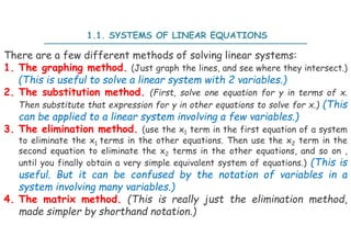
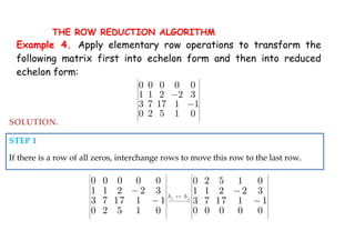
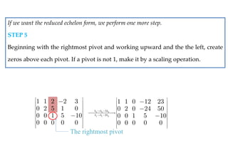
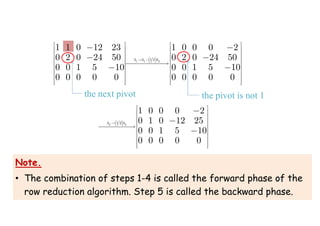
The document discusses systems of linear equations, defining linear equations and their solutions, and describing the conditions for consistency and equivalence of such systems. It covers various methods for solving linear systems, including graphing, substitution, elimination, and matrix methods. Additionally, the document introduces concepts of row reduction, echelon forms, and elementary row operations essential for simplifying matrices related to linear systems.

1. Chapter 1

2. 1.1
1.2
1.3
1.4
1.5

3. 1.1
Systems of linear equations

4. A linear equation in the variables is an equation that can be
written in the form
where b and the coefficients are real or complex numbers,
usually known in advance. The subscript n may be any positive integer.
1.1. SYSTEMS OF LINEAR EQUATIONS
1
, , n
x x

1 1 2 2 n n
a x a x a x b
   

1
, , n
a a

Example.
1 2
3
1 2
1 2 2
1/ 3 2
2 / 2 1 0
3/ 1
4 / 3 0
 
   
 
 
x y
x x
x x
x x x

5. The set of all possible solutions is called the solution set of the
linear system.
Two linear systems are called equivalent if they have the same
solution set.
1.1. SYSTEMS OF LINEAR EQUATIONS
A solution of the system is a list (s1, …, sn) of numbers that
makes each equation a true statement when the values s1, …, sn
are substituted for x1, …, xn.
A system of linear equation (or a linear system) is a collection
of one or more linear equations involving the same variables - say
x1, …, xn.

6.  How many solutions does a linear system have?
 How to find the solution of a linear system?
1.1. SYSTEMS OF LINEAR EQUATIONS

7.  
 
1 2
1 2
1 2
1 2
1 2
1 2
2 1
( )
3 3
2 1
2 3
2 1
2 1
x x
a
x x
x x
b
x x
x x
c
x x

  


  



  


  



  


  


1.1. SYSTEMS OF LINEAR EQUATIONS
Example 1. How many solutions do the following linear
systems have?

8. A system of linear equations has
1. no solution, or
2. exactly one solution, or
3. infinitely many solutions.
1.1. SYSTEMS OF LINEAR EQUATIONS
The linear system
is inconsistent.
The linear system
is consistent.

9. Example 2. Solve the linear system
1 2 3
1 2 3
2 3
2 0
2 4 6 4
3
x x x
x x x
x x

   


   


  



1.1. SYSTEMS OF LINEAR EQUATIONS

10. 1.1. SYSTEMS OF LINEAR EQUATIONS
There are a few different methods of solving linear systems:
1. The graphing method. (Just graph the lines, and see where they intersect.)
(This is useful to solve a linear system with 2 variables.)
2. The substitution method. (First, solve one equation for y in terms of x.
Then substitute that expression for y in other equations to solve for x.) (This
can be applied to a linear system involving a few variables.)
3. The elimination method. (use the x1 term in the first equation of a system
to eliminate the x1 terms in the other equations. Then use the x2 term in the
second equation to eliminate the x2 terms in the other equations, and so on ,
until you finally obtain a very simple equivalent system of equations.) (This is
useful. But it can be confused by the notation of variables in a
system involving many variables.)
4. The matrix method. (This is really just the elimination method,
made simpler by shorthand notation.)

11. Three basic operations are used to simplify a linear system:
• Replace one equation by the sum of itself and a multiple of
another equation,
• interchange two equations,
• multiply all the terms in an equation by a nonzero constant.
1.1. SYSTEMS OF LINEAR EQUATIONS
MATRIX NOTATION
An m x n matrix is a rectangular array of numbers with m rows and
n columns. In this case, size of the matrix is mxn.

12. 1.1. SYSTEMS OF LINEAR EQUATIONS
1 2 3
1 2 3
2 3
2 0
2 4 6 4
3
x x x
x x x
x x

   


   


  



1 2 1 0
2 4 6 4
0 1 1 3
 

 

 
 
 
1 2 1
2 4 6
0 1 1
 

 

 
 
 
Given linear system
with the coefficients of each variable aligned in columns,
the matrix is called the coefficient matrix (or matrix coefficients)
of the system, and
is called the augmented matrix of the system.

13. 1 2 3
1 2 3
2 3
2 0
2 4 6 4
3
x x x
x x x
x x

   


   


  



1 2 3
3
2 3
2 0
4 4
3
x x x
x
x x

   



 


  



1 2 3
3
2 3
2 0
1
3
x x x
x
x x

   



 


  



1 2 3
2 3
3
2 0
3
1
x x x
x x
x

   



  


 



1 2
2
3
2 1
2
1
x x
x
x

   



 


 



1
2
3
3
2
1
x
x
x

 



 


 



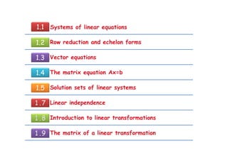
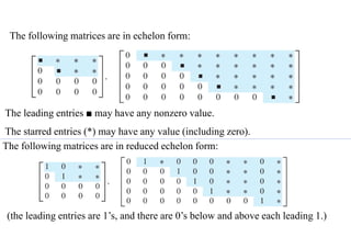
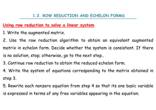
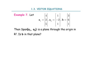
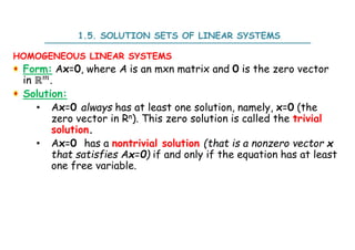
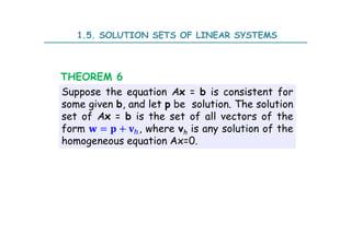
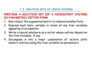
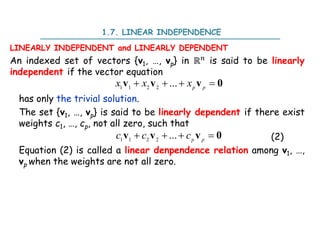
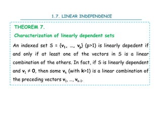
1.1. SYSTEMS OF LINEAR EQUATIONS
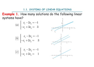
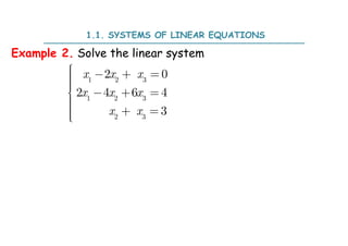
Example 2. Solve the linear system
Replace
[eq1] by
[eq1]-.[eq3]
Replace
[eq1]
by
[eq1]+
2.[eq2]
Replace
[eq2] by
[eq2]-2.[eq1]
Replace
[eq2] by
(1/4).[eq2]
Interchange
[eq2] and
[eq3]

14. ELEMENTARY ROW OPERATIONS:
1. (Replacement) Replace one row by the sum of itself and a
multiple of another row.
2. (Interchange) Interchange two rows.
3. (Scaling) Multiply all entries in a row by a nonzero constant.
1.1. SYSTEMS OF LINEAR EQUATIONS
 Row operations can be applied to any matrix, not merely to one
that arises as the augmented matrix of a linear system.
 Two matrices are called row equivalent if there is a sequence of
elementary row operations that transforms one matrix into the
other.
 If the augmented matrices of two linear systems are row
equivalent, then the two systems have the same solution set.

15. 1.2
Row reduction
and echelon forms

16. 1.2. ROW REDUCTION AND ECHELON FORMS
A nonzero or column in a matrix means a row or column that
contains at least one nonzero entry.
A leading entry of a row refers to the leftmost nonzero entry (in
a nonzero row).

17. ECHELON FORM
A rectangular matrix is in echelon form (or row echelon form (REF))
if it has the following three properties:
1. All nonzero rows are above any rows of all zeros.
2. Each leading entry of a row is in a column to the right of the
leading entry of the row above it.
3. All entries in a column below a leading entry are zeros.
If a matrix in echelon form satisfies the following additional
conditions, then it is in reduced (row) echelon form (RREF):
4. The leading entry in each nonzero row is 1.
5. Each leading 1 is the only nonzero entry in its column.
1.2. ROW REDUCTION AND ECHELON FORMS

18. 1.2. ROW REDUCTION AND ECHELON FORMS
An echelon matrix (respectively, reduced echelon matrix) is
one that is in echelon form (respectively, reduced echelon
form).
If a matrix A is row equivalent to an echelon matrix U, we call
U an echelon form (or row echelon form) of A; if U is a
reduced echelon form, we call U the reduced echelon form of
A.

19. The leading entries ■ may have any nonzero value.
The starred entries (*) may have any value (including zero).
The following matrices are in echelon form:
The following matrices are in reduced echelon form:
(the leading entries are 1’s, and there are 0’s below and above each leading 1.)

20. Example 3. Determine which matrices are in echelon form,
0 0
1 2
A
 
  
 
0 3 2
1 2 1
0 0 0
B
 
 

 
 
 
2 0 1
0 0 3
C
 
  
 
1 0 1
2 1 1
D
 
  

 

21. Example 3. Determine which matrices are in echelon form.
0 0
1 2
A
 
  
 
is NOT in echelon form.
0 3 2
1 2 1
0 0 0
B
 
 

 
 
 
is NOT in echelon form.
2 0 1
0 0 3
C
 
  
 
is in echelon form.
1 0 1
2 1 1
D
 
  

 
is NOT in echelon form.

22. A pivot position in a matrix A is a location in A that corresponds to
a leading 1 in the reduced echelon form of A. A pivot column is a
column of A that contains a pivot position.
A pivot is a nonzero number in a pivot position that is used as
needed to create zeros via row operations.
1.2. ROW REDUCTION AND ECHELON FORMS
Example.
1 2 1 1 2 1 1 2 1
2 4 1 0 0 1 0 0 1
1 2 3 0 0 4 0 0 0
1 2 1 1 2 0
0 0 1 0 0 1
0 0 0 0 0 0
  
     
     
   
     

     
     
  
   
    
   
   
   
A B
C
 
 

23. 1 4
0 0 0 0 0 0 2 5 1 0
1 1 2 2 3 1 1 2 2 3
3 7 17 1 1 3 7 17 1 1
0 2 5 1 0 0 0 0 0 0
h h
   
   
   
   
   

   
   
   
   
   
   
 
 

SOLUTION.
STEP 1
If there is a row of all zeros, interchange rows to move this row to the last row.
Example 4. Apply elementary row operations to transform the
following matrix first into echelon form and then into reduced
echelon form:
0 0 0 0 0
1 1 2 2 3
3 7 17 1 1
0 2 5 1 0
 
 
 
 
 
 
 
 
 
 
 
 


THE ROW REDUCTION ALGORITHM

24. 0 2 5 1 0
1 1 2 2 3
3 7 1 7 1 1
0 0 0 0 0
 
 
 
 
 
 
 
 
 
 
 


Pivot column
1 2
1 1 2 2 3
0 2 5 1 0
3 7 17 1 1
0 0 0 0 0
h h

 
 
 
 
 
   
  
 
 
 
 
 


Pivot
STEP 2
Begin with the leftmost, nonzero column. This is a pivot column. The pivot
position is at the top. Select a nonzero entry in the pivot column as a pivot.
If necessary, interchange rows to move this entry into the pivot position.
Pivot position

25. 1 1 2 2 3
0 2 5 1 0
3 7 1 7 1 1
0 0 0 0 0
 
 
 
 
 
 
 
 
 
 


Pivot
3 3 1
3
1 1 2 2 3
0 2 5 1 0
0 4 11 7 10
0 0 0 0 0
h h h
 
 
 
 
 
 
    
 
 
 
 
 


STEP 3
Use row replacement operations to create zeros in all positions below the pivot.

26. New pivot column
1 1 2 2 3
0 2 5 1 0
0 4 1 1 7 1 0
0 0 0 0 0
 
 
 
 
 
 
 
 
 
 


(new) pivot
3 3 2
2
1 1 2 2 3
0 2 5 1 0
0 0 1 5 10
0 0 0 0 0
h h h
 
 
 
 
 

  
 
 
 
 
 


STEP 4
Cover (or ignore) the row containing the pivot position and cover all rows, if
any, above it. Apply steps 1-3 to the submatrix that remains. Repear the process
until there are no more nonzero rows to modify..

27. 1 1 2 2 3
0 2 5 1 0
0 0 1 5 10
0 0 0 0 0
 
 
 
 
 
 
 
 
 
 


The rightmost pivot
2 2 3
1 1 3
5
2
1 1 0 12 23
0 2 0 24 50
0 0 1 5 10
0 0 0 0 0
h h h
h h h
 
 
 
 
 
 

  
 
 
 
 
 



If we want the reduced echelon form, we perform one more step.
STEP 5
Beginning with the rightmost pivot and working upward and the the left, create
zeros above each pivot. If a pivot is not 1, make it by a scaling operation.

28. 1 1 0 12 23
0 2 0 24 50
0 0 1 5 10
0 0 0 0 0
 
 
 
 
 
 
 
 
 
 



 
1 1 2
1 2
1 0 0 0 2
0 2 0 24 50
0 0 1 5 10
0 0 0 0 0
h h h
 
 
 
 
 

  
 
 
 
 
 



 
2 2
1 2
1 0 0 0 2
0 1 0 12 25
0 0 1 5 10
0 0 0 0 0
h h

 
 
 
 

  
 
 
 
 
 



the next pivot the pivot is not 1
Note.
• The combination of steps 1-4 is called the forward phase of the
row reduction algorithm. Step 5 is called the backward phase.

29. Example 5. Find the general solution of the system
1 2 3 4
1 2 3
2 2
2 1
x x x x
x x x
   


  

1.2. ROW REDUCTION AND ECHELON FORMS

30. 1.2. ROW REDUCTION AND ECHELON FORMS
Example 5. Find the general solution of the system
1 2 3 4
1 2 3
2 2
2 1
x x x x
x x x
   


  

Basic variable and Free variable.
A variable is a basic variable if it corresponds to a pivot column of
the augmented matrix of the system. Otherwise, the variable is
known as a free variable.
Note.
Whenever, a system is consistent, the solution set can be described
explicitly by solving the reduced system of equations for the basic
variables in terms of the free variables.

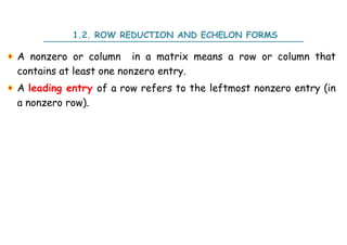
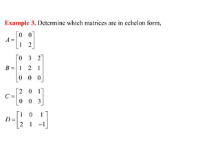
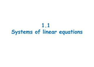
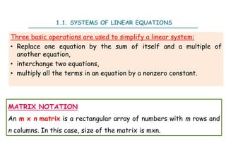
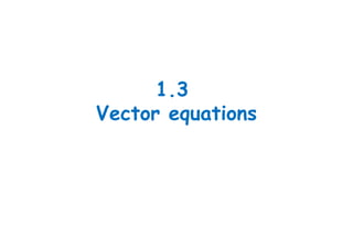
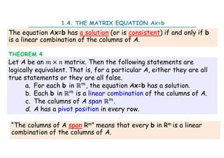
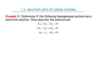
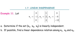
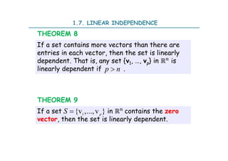
31. Existence and Uniqueness Theorem
A linear system is consistent the rightmost column of the
augmented matrix is not a pivot column—that is, if and only if an
echelon form of the augmented matrix has no row of the form
[0 … 0 b] with b nonzero.
If a linear system is consistent, then the solution set contains
either (i) a unique solution, when there are no free variables, or (ii)
infinitely many solution, when there is at least one free variable.
THEOREM 2
1.2. ROW REDUCTION AND ECHELON FORMS

32. Using row reduction to solve a linear system
1. Write the augmented matrix.
2. Use the row reduction algorithm to obtain an equivalent augmented
matrix in echelon form. Decide whether the system is consistent. If there
is no solution, stop; otherwise, go to the next step..
3. Continue row reduction to obtain the reduced echelon form.
4. Write the system of equations corresponding to the matrix obtained in
step 3.
5. Rewrite each nonzero equation from step 4 so that its one basic variable
is expressed in terms of any free variables appearing in the equation.
1.2. ROW REDUCTION AND ECHELON FORMS

33. 1.3
Vector equations

34. 1.3. VECTOR EQUATIONS
Vector in ℝ
A matrix with only one column is called a column vector, or simply
a vector.
is a vector with two entries, where w1 and w2 are any
real numbers.
The set of all vectors with two entries is denoted by R2.
1
2
w
w
w
 
  
 

35. Consider a rectangular coordinate
system in the plane. Because each
point in the plane is determined by
an ordered pair of numbers, we can
identify a geometric point (a,b) with
the column vector .
We may regard ℝ as the set of all
points in the plane.
1.3. VECTOR EQUATIONS
 
 
 
a
b

36. Parallelogram rule
for Addition
1.3. VECTOR EQUATIONS
Scalar multiple.
The set of all scalar multiples of one fixed
nonzero vector is a line through the vector
and the origin, (0,0).

37. Vectors in ℝ and Vector in ℝ
Vectors in ℝ are 3x1 column matrices with three entries. The
are represented geometrically by points in a three-dimensional
coordinate space.
If n is a positive integer, ℝ denotes the collection of all list of n
real numbers, usually written as nx1 column matrices , such as
The vector whose entries are all zero is called the zero vector
and is denoted by 0.
1.3. VECTOR EQUATIONS
1
2
u
n
u
u
u
 
 
 

 
 
 


38. 1.3. VECTOR EQUATIONS

39. LINEAR COMBINATIONS
Given vectors v , v , … ,v in ℝ and given scalars c , , … , , the
vector y defined by
is called a linear combination of v , v , … ,v with weight c , , … , .
The weights in a linear combination ca be any real numbers, including
zero.
1 1
...
   p p
c c
y v v
1.3. VECTOR EQUATIONS

40. Example 6. Let
Determine whether b can be generated (or written) as a linear
combination of a1 and a2.
(That is, determine whether weights x1 and x2 exist such that
x1a1 + x2a2 = b.)
a a b
1 2
1 3 3
2 , 0 , 6
3 1 7
     
 
     
     
  
     
     
 
     
     
1.3. VECTOR EQUATIONS

42. VECTOR EQUATION
A vector equation
has the same solution set as the linear system whose augmented
matrix is
(*)
In particular, b can be generated by a linear combination of a1, …,
an if and only if there exists a solution to the linear system
corresponding to the matrix (*)
1 1 2 2
a a ... a b
n n
x x x
   
 
1 2
a a a b
n

1.3. VECTOR EQUATIONS

43. SUBSET SPANNED BY GIVEN VECTORS
Let v , v , … ,v be in ℝ .
Subset of ℝ spanned (or generated) by v , v , … ,v
= Span v , v , … ,v
= the set of all linear combinations of v1, …, vp.
= the set of all vectors that can be written in the
form with c , , … , scalars.
1.3. VECTOR EQUATIONS
1 1 2 2
...
   p p
c c c
v v v
A set of vectors {v1,…, vp} in Rm spans (or generates) Rm if every
vector in Rm is a linear combination of v1,…, vp – that is, if
Span{v1,…, vp} = Rm.

44. If v is a nonzero vector in R3, then Span{v} is the line in R3
through v and 0.
If u and v are nonzero vectors in R3, with v not a multiple of u,
then Span{u, v} is the plane in R3 that contains u, v and 0.
A geometric description of Span{v} and Span{u,v}
1.3. VECTOR EQUATIONS

45. Example 7. Let
Then Span{a1, a2} is a plane through the origin in
R3. Is b in that plane?
a a b
1 2
4 1 3
2 , 2 , 6
5 1 1
     
     
     
   
     
     
     
     
1.3. VECTOR EQUATIONS

47. 1.4
The matrix equation
Ax=b

48. 1.4. THE MATRIX EQUATION Ax=b
The product Ax.
If A is an mxn matrix, with columns a1, …, an, and if x is in ℝ , then
the product of A and x, denoted by Ax, is linear combination of
the columns of A using the corresponding entries in x as weights;
that is,
.
Note that Ax is defined only if the number of columns of A equals
the number of entries in x.
 
1
2
1 2 1 1 2 2
a a a a a ... a
 
 
 
    
 
 
 
n n n
n
x
x
A x x x
x
x 


49. 1
2
3
4
1 2 3 4
0 1 2 3 ,
3 2 7 8
 
   
   
    
   
 
   
 
x
x
A
x
x
x

Ax

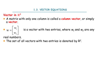
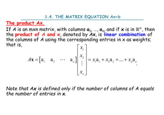
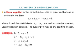
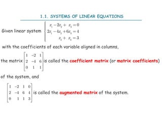
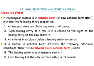
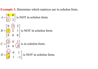
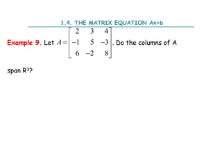
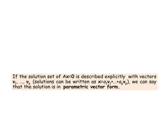
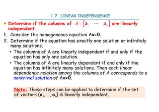
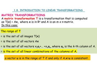
50. If A is an × matrix, with columns a1, …, an, and if b is in ℝ , the
matrix equation
Ax = b
has the same solution set as the vector equation
+ + ⋯ + =
which, in turn, has the same solution set as the system of linear
equations whose augmented matrix is
[ … b]
THEOREM 3
1.4. THE MATRIX EQUATION Ax=b

51. The equation Ax=b has a solution (or is consistent) if and only if b
is a linear combination of the columns of A.
Let A be an × matrix. Then the following statements are
logically equivalent. That is, for a particular A, either they are all
true statements or they are all false.
a. For each b in ℝ , the equation Ax=b has a solution.
b. Each b in ℝ is a linear combination of the columns of A.
c. The columns of A span ℝ .
d. A has a pivot position in every row.
THEOREM 4
1.4. THE MATRIX EQUATION Ax=b
“The columns of A span Rm” means that every b in Rm is a linear
combination of the columns of A.

52. Example 9. Let . Do the columns of A
span R3?
2 3 4
1 5 3
6 2 8
A
 
 
  
 

 
 
1.4. THE MATRIX EQUATION Ax=b

53. If A is an × matrix, u and v are vectors in
ℝ , and c is a scalar, then:
a. A(u + v) = Au + Av;
b. A(cu) = c(Au).
THEOREM 5
1.4. THE MATRIX EQUATION Ax=b

54. 1.5
Solution sets of linear systems

55. 1.5. SOLUTION SETS OF LINEAR SYSTEMS
HOMOGENEOUS LINEAR SYSTEMS
Form: Ax=0, where A is an mxn matrix and 0 is the zero vector
in ℝ .
Solution:
• Ax=0 always has at least one solution, namely, x=0 (the
zero vector in Rn). This zero solution is called the trivial
solution.
• Ax=0 has a nontrivial solution (that is a nonzero vector x
that satisfies Ax=0) if and only if the equation has at least
one free variable.

56. 1.5. SOLUTION SETS OF LINEAR SYSTEMS
Example 9. Determine if the following homogeneous system has a
nontrivial solution. Then describe the solution set.
1 2 3
1 2 3
1 2 3
3 5 4 0
3 2 4 0
6 8 0
x x x
x x x
x x x
  
   
  

58. If the solution set of Ax=0 is described explicitly with vectors
v1, …, vp (solutions can be written as x=a1v1+…+apvp), we can say
that the solution is in parametric vector form.

59. 1.5. SOLUTION SETS OF LINEAR SYSTEMS
Example 10. Describe all solutions of Ax = b, where
and
3 5 4
3 2 4
6 1 8
A

 
 
  
 

 
 
7
b 1
4
 
 
 
 

 
 

62. 1.5. SOLUTION SETS OF LINEAR SYSTEMS
Suppose the equation Ax = b is consistent for
some given b, and let p be solution. The solution
set of Ax = b is the set of all vectors of the
form = + , where vh is any solution of the
homogeneous equation Ax=0.
THEOREM 6

63. 1.5. SOLUTION SETS OF LINEAR SYSTEMS
WRITING A SOLUTION SET (OF A CONSISTENT SYSTEM)
IN PARAMETRIC VECTOR FORM
1. Row reduce the augmented matrix to reduced echelon form.
2. Express each basic variable in terms of any free variables
appearing in an equation.
3. Write a typical solution x as a vector whose entries depend on
the free variables, if any.
4. Decompose x into a linear combination of vectors (with
numeric entries) using the free variables as parameters.

64. 1.7
Linear independence

65. 1.7. LINEAR INDEPENDENCE
LINEARLY INDEPENDENT and LINEARLY DEPENDENT
Consider the vector equation
1 1 2 2
v v ... v 0
p p
x x x
   

66. 1.7. LINEAR INDEPENDENCE
LINEARLY INDEPENDENT and LINEARLY DEPENDENT
An indexed set of vectors {v1, …, vp} in ℝ is said to be linearly
independent if the vector equation
has only the trivial solution.
The set {v1, …, vp} is said to be linearly dependent if there exist
weights c1, …, cp, not all zero, such that
(2)
Equation (2) is called a linear denpendence relation among v1, …,
vp when the weights are not all zero.
1 1 2 2
...
   
p p
x x x
v v v 0
1 1 2 2
...
   
p p
c c c
v v v 0

67. 1.7. LINEAR INDEPENDENCE
Example 11. Let
a. Determine if the set {v1, v2, v3} is linearly independent.
b. If possible, find a linear dependence relation among v1, v2 and v3.
1 2 3
3 1 3
1 , 2 , 8
0 4 12
     
     
     
    
     
     

     
     
v v v

70. 1.7. LINEAR INDEPENDENCE
Determine if the columns of are linearly
independent.
1. Consider the homogeneous equation Ax=0.
2. Determine if the equation has exactly one solution or infinitely
many solutions.
• The columns of A are linearly independent if and only if the
equation has only one solution.
• The columns of A are linearly dependent if and only if the
equation has infinitely many solutions. Then each linear
dependence relation among the columns of A corresponds to a
nontrivial solution of Ax=0.
 
1
 n
A a a

Note: These steps can be applied to determine if the set
of vectors {a1, …, an} is linearly independent.

71. 1.7. LINEAR INDEPENDENCE
 {v} is linearly independent if and only if v ≠ 0.
 {v} is linearly dependent if and only if v = 0.
NOTES
 {v1, v2} is linearly independent if and only if neither of the
vectors is a multiple of the other.
 {v1, v2} is linearly dependent if and only if at least one of
the vectors is a multiple of the other.

72. 1.7. LINEAR INDEPENDENCE
THEOREM 7.
Characterization of linearly dependent sets
An indexed set S = {v1, …, vp} (p>1) is linearly depedent if
and only if at least one of the vectors in S is a linear
combination of the others. In fact, if S is linearly dependent
and v1 ≠ 0, then some vk (with k>1) is a linear combination of
the preceding vectors v1, …, vk-1.

73. 1.7. LINEAR INDEPENDENCE
If a set contains more vectors than there are
entries in each vector, then the set is linearly
dependent. That is, any set {v1, …, vp} in ℝ is
linearly dependent if .
THEOREM 8
p n

If a set in ℝ contains the zero
vector, then the set is linearly dependent.
THEOREM 9
1
{v ,...,v }
p
S 

74. 1.7. LINEAR INDEPENDENCE
Example 12. Determine by inspection if the given set is linearly
dependent 1 2
2 1 2 0 6 0 1
3 6
. 1 , 1 , 7 , 1 ; . 0 , 0 , 2 ; . ,
1 2
0 1 9 2 2 0 8
4 8
a b c
   
                 
 
                 
                 
                 

                 
                 
                 
   

75. 1.8
Introduction to linear
transformations

76. 1.8. INTRODUCTION TO LINEAR TRANSFORMATIONS

77. 1.8. INTRODUCTION TO LINEAR TRANSFORMATIONS

78. A transformation (or function or mapping) T from ℝ to ℝ is a
rule that assigns to each vector x in ℝ a vector T (x) in ℝ .
ℝ : the domain of T
ℝ : the codomain of T.
Notation: : ℝ → ℝ
1.8. INTRODUCTION TO LINEAR TRANSFORMATIONS
For x in ℝ , vector T(x) in
ℝ is called the image of x
(under the action of T).
The set of all images T (x)
is called the range of T.

79. MATRIX TRANSFORMATIONS
A matrix transformation T is a transformation that is computed
as T(x) = Ax, where x is in Rn and A is an m x n matrix.
In this case:
The range of T
= is the set of all images T(x)
= is the set of all vectors Ax
= is the set of all vectors x1a1+… +xnan, where ak is the k-th column of A.
= is the set of all linear combinations of the columns of A.
1.8. INTRODUCTION TO LINEAR TRANSFORMATIONS
a vector u is in the range of T if and only if A.x=u is consistent.

80. Example 13. Let
and define a transformation T: R 2 -> R3 by T(x) = Ax.
a. Find the image of u under the transformation T.
b. Find an x in R2 whose image under T is b.
c. Is there more than one x whose image under T is b?
d. Determine if c is in the range of the transformation T.
2 1 3 1
3
1 1 , , 3 , 1
2
3 5 1 1
A
     
     
 
     
 
     
     
 
     
 
 
     
     
u b c
1.8. INTRODUCTION TO LINEAR TRANSFORMATIONS

81. a. Find the image of u under the
transformation T.
2 1 3 1
3
1 1 , , 3 , 1
2
3 5 1 1
A
     
     
 
     
 
     
     
 
     
 
 
     
     
u b c
T(x) = Ax.

82. 2 1 3 1
3
1 1 , , 3 , 1
2
3 5 1 1
A
     
     
 
     
 
     
     
 
     
 
 
     
     
u b c
b. Find an x in R2 whose image under T is b.
T(x) = Ax.

83. c. Is there more than one x whose image under T is b?

84. 2 1 3 1
3
1 1 , , 3 , 1
2
3 5 1 1
A
     
     
 
     
 
     
     
 
     
 
 
     
     
u b c
d. Determine if c is in the range of the
transformation T.
T(x) = Ax.

85. Linear transformations
A transformation (or mapping) T is linear if:
i. for all u, v in the domain of T;
ii. for all scalars c an all u in the domain of T.
(u v) (u) (v)
T T T
  
( u) (u)
T c cT

1.8. INTRODUCTION TO LINEAR TRANSFORMATIONS
If T is a linear transformation, then T(0) = 0.
T is a linear transformation if and only if
(*)
for all vectors u, v in the domain of T and all scalars c, d.
Repeated application of (*) produces a useful generalization:
( u v) (u) (v)
T c d cT dT
  
1 1 1 1
( v ... v ) (v ) ... (v )
p p p p
T c c cT c T
    

86. Example 14. Given a scalar r, define T: R2 -> R2 by T(x) = rx.
T is called a contraction when , and a dilation when .
Let r = 5, and show that T is a linear transformation.
0 1
r
  1
r 
1.8. INTRODUCTION TO LINEAR TRANSFORMATIONS

87. 1.9
The matrix of a linear
transformation

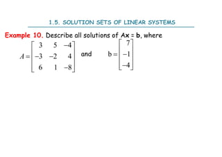
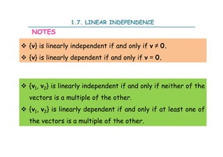
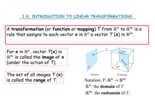
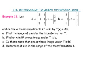
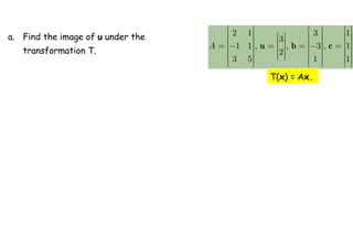
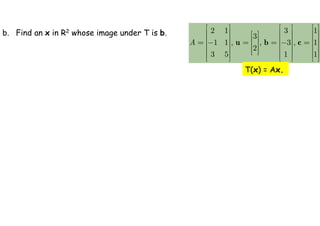
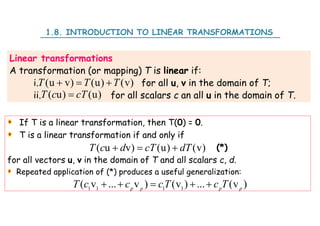
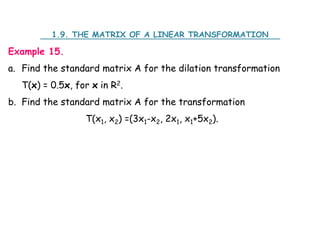
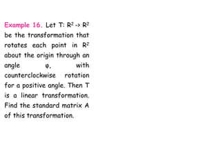
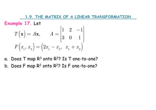
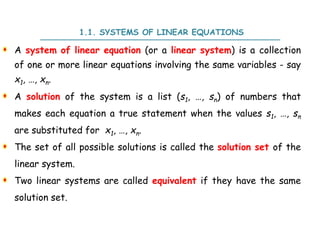
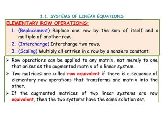
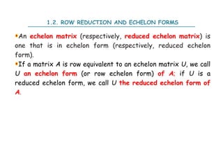
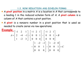
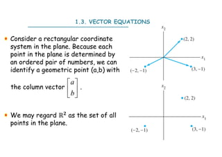
88. 1.9. THE MATRIX OF A LINEAR TRANSFORMATION
THEOREM 10.
Let T: Rn -> Rm be a linear transformation. Then there exists a unique
matrix A such that
T(x) = Ax for all x in Rn.
In fact, A is the m x n matrix whose k-th is the vector T(ek), where ek
is the k-th column of the identity matrix in Rn).
A = [T(e1) T(e2) …………. T(en)]
The matrix A is called the standard matrix for the linear
transformation T.
The nxn identity matrix In is (the identity matrix in Rn), is the nxn
matrix with 1’s on the diagonal and 0’s elsewhere.

89. Example 15.
a. Find the standard matrix A for the dilation transformation
T(x) = 0.5x, for x in R2.
b. Find the standard matrix A for the transformation
T(x1, x2) =(3x1-x2, 2x1, x1+5x2).
1.9. THE MATRIX OF A LINEAR TRANSFORMATION

90. Example 16. Let T: R2 -> R2
be the transformation that
rotates each point in R2
about the origin through an
angle φ, with
counterclockwise rotation
for a positive angle. Then T
is a linear transformation.
Find the standard matrix A
of this transformation.

91. Geometric linear transformation of R2
• See pages 74-76.
1.9. THE MATRIX OF A LINEAR TRANSFORMATION

92. One-to-one and Onto Mappings.
A mapping T: Rn -> Rm is said to be
1. onto Rm if each b in Rm is the image of at least one x in Rn.
2. one-to-one if each b in Rm is the image of at most one x in Rn.
1.9. THE MATRIX OF A LINEAR TRANSFORMATION
Remark:
Suppose Amxn is the standard matrix for the linear transformation
T: Rn -> Rm. Then
1. T maps Rn onto Rm if and only if A has a pivot position in every row.
2. T is one-to-one if and only if A has a pivot position in every column.

93. Example 17. Let
a. Does T map R3 onto R2? Is T one-to-one?
b. Does F map R2 onto R2? Is F one-to-one?
 
   
1 2 1 2 1 2
1 2 1
,
3 0 1
, 2 ,
T A A
F x x x x x x
 

 
   
 
 
  
x x
1.9. THE MATRIX OF A LINEAR TRANSFORMATION