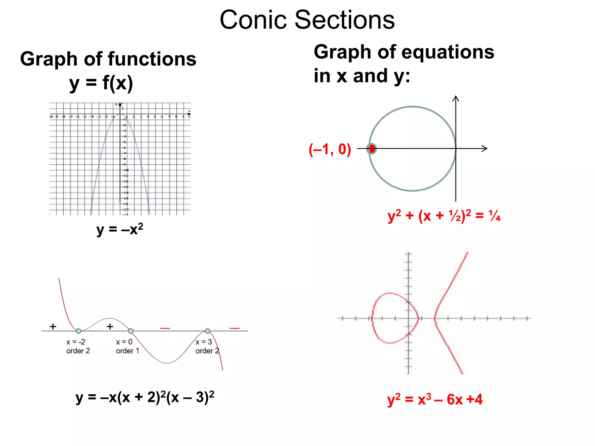
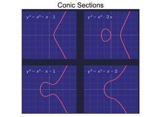
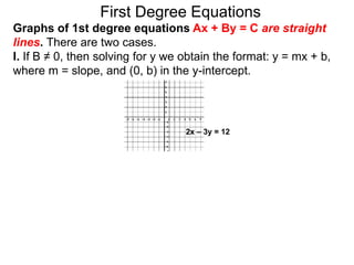
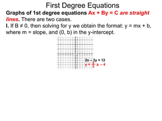
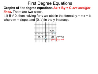
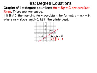
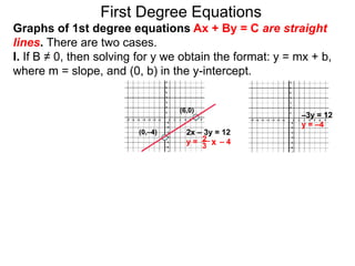
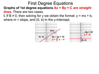
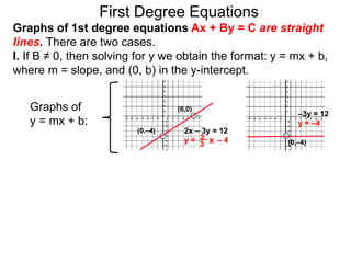
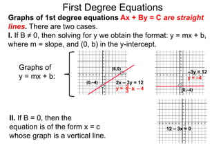
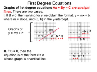
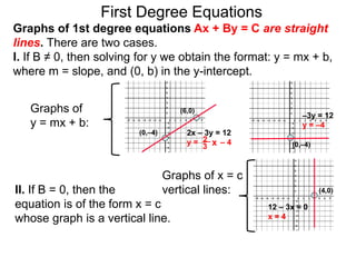
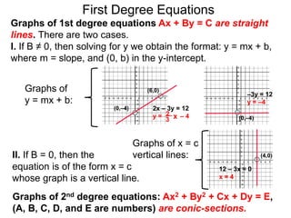
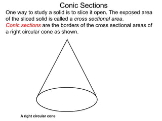
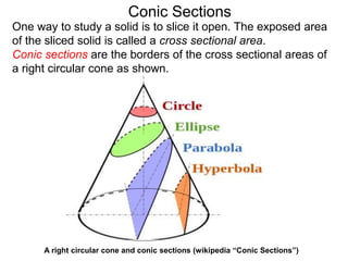
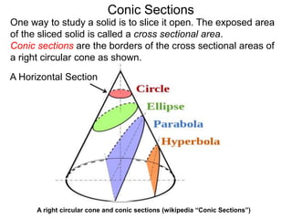
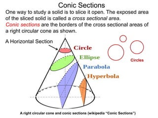
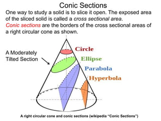
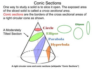
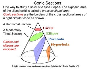
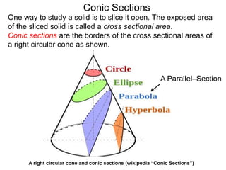
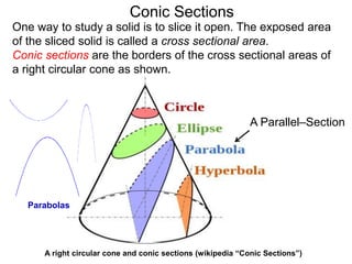
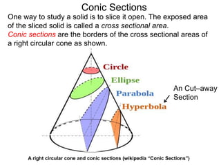
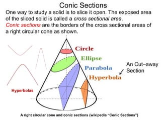
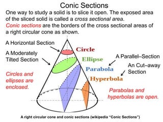
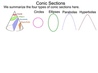
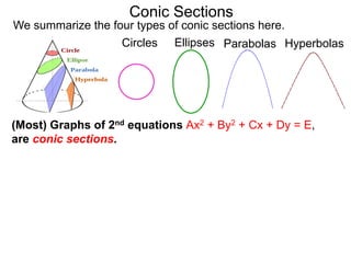
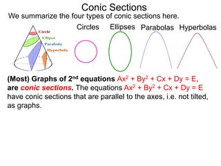
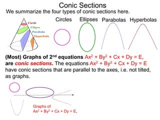
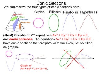
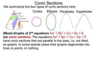
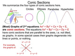
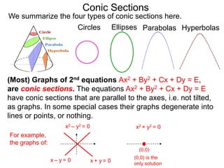
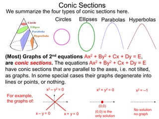
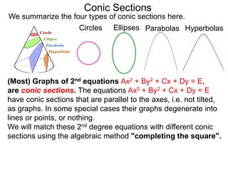
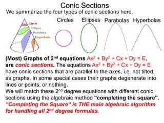
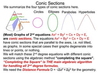
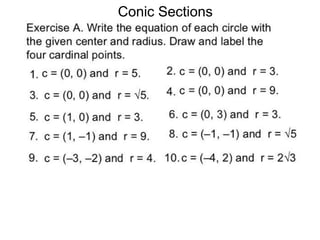
SlideShare a Scribd company logo
Conic Sections
y2 + (x + ½)2 = ¼
(–1, 0)
Graph of equations
in x and y:
Graph of functions
y = f(x)
y = –x2
y = –x(x + 2)2(x – 3)2
y2 = x3 – 6x +4
Conic Sections
First Degree Equations
Graphs of 1st degree equations Ax + By = C are straight
lines.
First Degree Equations
Graphs of 1st degree equations Ax + By = C are straight
lines. There are two cases.
First Degree Equations
Graphs of 1st degree equations Ax + By = C are straight
lines. There are two cases.
I. If B ≠ 0, then solving for y we obtain the format: y = mx + b,
where m = slope, and (0, b) in the y-intercept.
First Degree Equations
Graphs of 1st degree equations Ax + By = C are straight
lines. There are two cases.
I. If B ≠ 0, then solving for y we obtain the format: y = mx + b,
where m = slope, and (0, b) in the y-intercept.
2x – 3y = 12
First Degree Equations
Graphs of 1st degree equations Ax + By = C are straight
lines. There are two cases.
I. If B ≠ 0, then solving for y we obtain the format: y = mx + b,
where m = slope, and (0, b) in the y-intercept.
2x – 3y = 12
y = – 4
2 x
3
First Degree Equations
Graphs of 1st degree equations Ax + By = C are straight
lines. There are two cases.
I. If B ≠ 0, then solving for y we obtain the format: y = mx + b,
where m = slope, and (0, b) in the y-intercept.
(6,0)
(0,–4) 2x – 3y = 12
y = – 4
2 x
3
First Degree Equations
Graphs of 1st degree equations Ax + By = C are straight
lines. There are two cases.
I. If B ≠ 0, then solving for y we obtain the format: y = mx + b,
where m = slope, and (0, b) in the y-intercept.
(6,0)
(0,–4) 2x – 3y = 12
y = – 4
2 x
3
First Degree Equations
Graphs of 1st degree equations Ax + By = C are straight
lines. There are two cases.
I. If B ≠ 0, then solving for y we obtain the format: y = mx + b,
where m = slope, and (0, b) in the y-intercept.
(6,0)
(0,–4)
–3y = 12
y = –4
2x – 3y = 12
y = – 4
2 x
3
First Degree Equations
Graphs of 1st degree equations Ax + By = C are straight
lines. There are two cases.
I. If B ≠ 0, then solving for y we obtain the format: y = mx + b,
where m = slope, and (0, b) in the y-intercept.
(6,0)
(0,–4)
–3y = 12
y = –4
2x – 3y = 12
y = – 4
2 x
3 (0,–4)
Graphs of
y = mx + b:
First Degree Equations
Graphs of 1st degree equations Ax + By = C are straight
lines. There are two cases.
I. If B ≠ 0, then solving for y we obtain the format: y = mx + b,
where m = slope, and (0, b) in the y-intercept.
(6,0)
(0,–4)
–3y = 12
y = –4
2x – 3y = 12
y = – 4
2 x
3
Il. If B = 0, then the
equation is of the form x = c
whose graph is a vertical line.
12 – 3x = 0
(0,–4)
Graphs of
y = mx + b:
First Degree Equations
Graphs of 1st degree equations Ax + By = C are straight
lines. There are two cases.
I. If B ≠ 0, then solving for y we obtain the format: y = mx + b,
where m = slope, and (0, b) in the y-intercept.
(6,0)
(0,–4)
–3y = 12
y = –4
2x – 3y = 12
y = – 4
2 x
3
Il. If B = 0, then the
equation is of the form x = c
whose graph is a vertical line.
12 – 3x = 0
x = 4
(0,–4)
Graphs of
y = mx + b:
First Degree Equations
Graphs of 1st degree equations Ax + By = C are straight
lines. There are two cases.
I. If B ≠ 0, then solving for y we obtain the format: y = mx + b,
where m = slope, and (0, b) in the y-intercept.
(6,0)
(0,–4)
–3y = 12
y = –4
2x – 3y = 12
y = – 4
2 x
3
Il. If B = 0, then the
equation is of the form x = c
whose graph is a vertical line.
12 – 3x = 0
x = 4
Graphs of x = c
vertical lines:
(0,–4)
(4,0)
Graphs of
y = mx + b:
First Degree Equations
Graphs of 1st degree equations Ax + By = C are straight
lines. There are two cases.
I. If B ≠ 0, then solving for y we obtain the format: y = mx + b,
where m = slope, and (0, b) in the y-intercept.
(6,0)
(0,–4)
–3y = 12
y = –4
2x – 3y = 12
y = – 4
2 x
3
Il. If B = 0, then the
equation is of the form x = c
whose graph is a vertical line.
12 – 3x = 0
x = 4
Graphs of x = c
vertical lines:
Graphs of 2nd degree equations: Ax2 + By2 + Cx + Dy = E,
(A, B, C, D, and E are numbers) are conic-sections.
(0,–4)
(4,0)
Conic Sections
One way to study a solid is to slice it open.
Conic Sections
One way to study a solid is to slice it open. The exposed area
of the sliced solid is called a cross sectional area.
Conic Sections
A right circular cone
One way to study a solid is to slice it open. The exposed area
of the sliced solid is called a cross sectional area.
Conic sections are the borders of the cross sectional areas of
a right circular cone as shown.
Conic Sections
A right circular cone and conic sections (wikipedia “Conic Sections”)
One way to study a solid is to slice it open. The exposed area
of the sliced solid is called a cross sectional area.
Conic sections are the borders of the cross sectional areas of
a right circular cone as shown.
Conic Sections
A Horizontal Section
A right circular cone and conic sections (wikipedia “Conic Sections”)
One way to study a solid is to slice it open. The exposed area
of the sliced solid is called a cross sectional area.
Conic sections are the borders of the cross sectional areas of
a right circular cone as shown.
Circles
Conic Sections
A Moderately
Tilted Section
A right circular cone and conic sections (wikipedia “Conic Sections”)
One way to study a solid is to slice it open. The exposed area
of the sliced solid is called a cross sectional area.
Conic sections are the borders of the cross sectional areas of
a right circular cone as shown.
Ellipses
Conic Sections
A Horizontal Section
A Moderately
Tilted Section
A right circular cone and conic sections (wikipedia “Conic Sections”)
One way to study a solid is to slice it open. The exposed area
of the sliced solid is called a cross sectional area.
Conic sections are the borders of the cross sectional areas of
a right circular cone as shown.
Circles and
ellipses are
enclosed.
Conic Sections
A right circular cone and conic sections (wikipedia “Conic Sections”)
A Parallel–Section
One way to study a solid is to slice it open. The exposed area
of the sliced solid is called a cross sectional area.
Conic sections are the borders of the cross sectional areas of
a right circular cone as shown.
Parabolas
Conic Sections
A right circular cone and conic sections (wikipedia “Conic Sections”)
One way to study a solid is to slice it open. The exposed area
of the sliced solid is called a cross sectional area.
Conic sections are the borders of the cross sectional areas of
a right circular cone as shown.
An Cut–away
Section
Hyperbolas
Conic Sections
A right circular cone and conic sections (wikipedia “Conic Sections”)
An Cut–away
Section
One way to study a solid is to slice it open. The exposed area
of the sliced solid is called a cross sectional area.
Conic sections are the borders of the cross sectional areas of
a right circular cone as shown.
Parabolas and
hyperbolas are open.
A Horizontal Section
A Moderately
Tilted Section
Circles and
ellipses are
enclosed.
A Parallel–Section
Conic Sections
Circles Ellipses Parabolas Hyperbolas
We summarize the four types of conic sections here.
Conic Sections
Circles Ellipses Parabolas Hyperbolas
We summarize the four types of conic sections here.
(Most) Graphs of 2nd equations Ax2 + By2 + Cx + Dy = E,
are conic sections.
Conic Sections
(Most) Graphs of 2nd equations Ax2 + By2 + Cx + Dy = E,
are conic sections. The equations Ax2 + By2 + Cx + Dy = E
have conic sections that are parallel to the axes, i.e. not tilted,
as graphs.
Circles Ellipses Parabolas Hyperbolas
We summarize the four types of conic sections here.
Conic Sections
(Most) Graphs of 2nd equations Ax2 + By2 + Cx + Dy = E,
are conic sections. The equations Ax2 + By2 + Cx + Dy = E
have conic sections that are parallel to the axes, i.e. not tilted,
as graphs.
Circles Ellipses Parabolas Hyperbolas
We summarize the four types of conic sections here.
Graphs of
Ax2 + By2 + Cx + Dy = E,
Conic Sections
(Most) Graphs of 2nd equations Ax2 + By2 + Cx + Dy = E,
are conic sections. The equations Ax2 + By2 + Cx + Dy = E
have conic sections that are parallel to the axes, i.e. not tilted,
as graphs. In some special cases their graphs degenerate into
lines or points, or nothing.
Circles Ellipses Parabolas Hyperbolas
We summarize the four types of conic sections here.
x2 – y2 = 0
For example,
the graphs of:
x + y = 0
x – y = 0
x2 + y2 = 0
(0,0)
(0,0) is the
only solution
Conic Sections
(Most) Graphs of 2nd equations Ax2 + By2 + Cx + Dy = E,
are conic sections. The equations Ax2 + By2 + Cx + Dy = E
have conic sections that are parallel to the axes, i.e. not tilted,
as graphs. In some special cases their graphs degenerate into
lines or points, or nothing.
Circles Ellipses Parabolas Hyperbolas
We summarize the four types of conic sections here.
x2 – y2 = 0
For example,
the graphs of:
x + y = 0
x – y = 0
x2 = –1
x2 + y2 = 0
(0,0)
(0,0) is the
only solution
No solution
no graph
Conic Sections
(Most) Graphs of 2nd equations Ax2 + By2 + Cx + Dy = E,
are conic sections. The equations Ax2 + By2 + Cx + Dy = E
have conic sections that are parallel to the axes, i.e. not tilted,
as graphs. In some special cases their graphs degenerate into
lines or points, or nothing.
We will match these 2nd degree equations with different conic
sections using the algebraic method "completing the square".
Circles Ellipses Parabolas Hyperbolas
We summarize the four types of conic sections here.
Conic Sections
(Most) Graphs of 2nd equations Ax2 + By2 + Cx + Dy = E,
are conic sections. The equations Ax2 + By2 + Cx + Dy = E
have conic sections that are parallel to the axes, i.e. not tilted,
as graphs. In some special cases their graphs degenerate into
lines or points, or nothing.
We will match these 2nd degree equations with different conic
sections using the algebraic method "completing the square".
“Completing the Square“ is THE main algebraic algorithm
for handling all 2nd degree formulas.
We need the Distance Formula D = Δx2 + Δy2 for the geometry.
Circles Ellipses Parabolas Hyperbolas
We summarize the four types of conic sections here.
Circles
A circle is the set of all the points that have equal distance r,
called the radius, to a fixed point C which is called the center.
Circles
A circle is the set of all the points that have equal distance r,
called the radius, to a fixed point C which is called the center.
C
r
r
Circles
A circle is the set of all the points that have equal distance r,
called the radius, to a fixed point C which is called the center.
C
r
r
Circles
A circle is the set of all the points that have equal distance r,
called the radius, to a fixed point C which is called the center.
C
r
r
The radius and the center completely determine the circle.
Circles
A circle is the set of all the points that have equal distance r,
called the radius, to a fixed point C which is called the center.
C
r
The radius and the center completely determine the circle.
Circles
Let (h, k) be the center of a
circle and r be the radius.
(h, k)
A circle is the set of all the points that have equal distance r,
called the radius, to a fixed point C which is called the center.
r
C
r
The radius and the center completely determine the circle.
Circles
(x, y)
Let (h, k) be the center of a
circle and r be the radius.
Suppose (x, y) is a point on
the circle, then the distance
between (x, y) and the center
is r.
(h, k)
A circle is the set of all the points that have equal distance r,
called the radius, to a fixed point C which is called the center.
r
C
r
The radius and the center completely determine the circle.
Circles
(x, y)
Let (h, k) be the center of a
circle and r be the radius.
Suppose (x, y) is a point on
the circle, then the distance
between (x, y) and the center
is r. Hence,
(h, k)
r =  (x – h)2 + (y – k)2
or
r2 = (x – h)2 + (y – k)2
This is called the standard form of circles.
A circle is the set of all the points that have equal distance r,
called the radius, to a fixed point C which is called the center.
r
C
r
The radius and the center completely determine the circle.
Circles
(x, y)
Let (h, k) be the center of a
circle and r be the radius.
Suppose (x, y) is a point on
the circle, then the distance
between (x, y) and the center
is r. Hence,
(h, k)
r =  (x – h)2 + (y – k)2
or
r2 = (x – h)2 + (y – k)2
This is called the standard form of circles. Given an equation
of this form, we can easily identify the center and the radius.
A circle is the set of all the points that have equal distance r,
called the radius, to a fixed point C which is called the center.
r
C
r2 = (x – h)2 + (y – k)2
Circles
r2 = (x – h)2 + (y – k)2
must be “ – ”
Circles
r2 = (x – h)2 + (y – k)2
r is the radius must be “ – ”
Circles
r2 = (x – h)2 + (y – k)2
r is the radius must be “ – ”
(h, k) is the center
Circles
r2 = (x – h)2 + (y – k)2
r is the radius must be “ – ”
(h, k) is the center
Circles
Example B. Write the equation
of the circle as shown.
(–1, 3)
r2 = (x – h)2 + (y – k)2
r is the radius must be “ – ”
(h, k) is the center
Circles
Example B. Write the equation
of the circle as shown.
The center is (–1, 3)
and the radius is 5. (–1, 3)
r2 = (x – h)2 + (y – k)2
r is the radius must be “ – ”
(h, k) is the center
Circles
Example B. Write the equation
of the circle as shown.
The center is (–1, 3)
and the radius is 5.
Hence the equation is:
52 = (x – (–1))2 + (y – 3)2
(–1, 3)
r2 = (x – h)2 + (y – k)2
r is the radius must be “ – ”
(h, k) is the center
Circles
Example B. Write the equation
of the circle as shown.
The center is (–1, 3)
and the radius is 5.
Hence the equation is:
52 = (x – (–1))2 + (y – 3)2
or
25 = (x + 1)2 + (y – 3 )2
(–1, 3)
Example C. Identify the center and
the radius of 16 = (x – 3)2 + (y + 2)2.
Label the top, bottom, left and right
most points. Graph it.
Circles
Example C. Identify the center and
the radius of 16 = (x – 3)2 + (y + 2)2.
Label the top, bottom, left and right
most points. Graph it.
Put 16 = (x – 3)2 + (y + 2)2 into the
standard form:
42 = (x – 3)2 + (y – (–2))2
Circles
Example C. Identify the center and
the radius of 16 = (x – 3)2 + (y + 2)2.
Label the top, bottom, left and right
most points. Graph it.
Put 16 = (x – 3)2 + (y + 2)2 into the
standard form:
42 = (x – 3)2 + (y – (–2))2
Hence r = 4, center = (3, –2)
Circles
Example C. Identify the center and
the radius of 16 = (x – 3)2 + (y + 2)2.
Label the top, bottom, left and right
most points. Graph it.
Put 16 = (x – 3)2 + (y + 2)2 into the
standard form:
42 = (x – 3)2 + (y – (–2))2
Hence r = 4, center = (3, –2)
(3,–2)
Circles
r = 4
Example C. Identify the center and
the radius of 16 = (x – 3)2 + (y + 2)2.
Label the top, bottom, left and right
most points. Graph it.
Put 16 = (x – 3)2 + (y + 2)2 into the
standard form:
42 = (x – 3)2 + (y – (–2))2
Hence r = 4, center = (3, –2)
(3,–2)
Circles
r = 4
Example C. Identify the center and
the radius of 16 = (x – 3)2 + (y + 2)2.
Label the top, bottom, left and right
most points. Graph it.
Put 16 = (x – 3)2 + (y + 2)2 into the
standard form:
42 = (x – 3)2 + (y – (–2))2
Hence r = 4, center = (3, –2)
(3,–2)
Circles
When equations are not in the standard form, we have to
rearrange them into the standard form. We do this by
"completing the square".
To complete the square means to add a number to an
expression so the sum is a perfect square.
r = 4
Example C. Identify the center and
the radius of 16 = (x – 3)2 + (y + 2)2.
Label the top, bottom, left and right
most points. Graph it.
Put 16 = (x – 3)2 + (y + 2)2 into the
standard form:
42 = (x – 3)2 + (y – (–2))2
Hence r = 4, center = (3, –2)
(3,–2)
Circles
When equations are not in the standard form, we have to
rearrange them into the standard form. We do this by
"completing the square".
To complete the square means to add a number to an
expression so the sum is a perfect square. This procedure is
the main technique in dealing with 2nd degree equations.
r = 4
(Completing the Square)
Circles
(Completing the Square)
Circles
Example D. Fill in the blank to make a perfect square.
a. x2 – 6x + (–6/2)2 = x2 – 6x + 9 = (x – 3)2
b. y2 + 12y + (12/2)2 = y2 + 12y + 36 = ( y + 6)2
(Completing the Square)
If we are given x2 + bx, then adding (b/2)2 to the expression
makes the expression a perfect square,
Circles
Example D. Fill in the blank to make a perfect square.
a. x2 – 6x + (–6/2)2 = x2 – 6x + 9 = (x – 3)2
b. y2 + 12y + (12/2)2 = y2 + 12y + 36 = ( y + 6)2
(Completing the Square)
If we are given x2 + bx, then adding (b/2)2 to the expression
makes the expression a perfect square,
Circles
Example D. Fill in the blank to make a perfect square.
a. x2 – 6x + (–6/2)2
b. y2 + 12y + (12/2)2 = y2 + 12y + 36 = ( y + 6)2
(Completing the Square)
If we are given x2 + bx, then adding (b/2)2 to the expression
makes the expression a perfect square,
Circles
Example D. Fill in the blank to make a perfect square.
a. x2 – 6x + (–6/2)2 = x2 – 6x + 9 = (x – 3)2
b. y2 + 12y + (12/2)2 = y2 + 12y + 36 = ( y + 6)2
(Completing the Square)
If we are given x2 + bx, then adding (b/2)2 to the expression
makes the expression a perfect square, i.e. x2 + bx + (b/2)2
is the perfect square (x + b/2)2.
Circles
Example D. Fill in the blank to make a perfect square.
a. x2 – 6x + (–6/2)2 = x2 – 6x + 9 = (x – 3)2
b. y2 + 12y + (12/2)2
(Completing the Square)
If we are given x2 + bx, then adding (b/2)2 to the expression
makes the expression a perfect square, i.e. x2 + bx + (b/2)2
is the perfect square (x + b/2)2.
Circles
Example D. Fill in the blank to make a perfect square.
a. x2 – 6x + (–6/2)2 = x2 – 6x + 9 = (x – 3)2
b. y2 + 12y + (12/2)2 = y2 + 12y + 36
(Completing the Square)
If we are given x2 + bx, then adding (b/2)2 to the expression
makes the expression a perfect square, i.e. x2 + bx + (b/2)2
is the perfect square (x + b/2)2.
Circles
Example D. Fill in the blank to make a perfect square.
a. x2 – 6x + (–6/2)2 = x2 – 6x + 9 = (x – 3)2
b. y2 + 12y + (12/2)2 = y2 + 12y + 36 = ( y + 6)2
(Completing the Square)
If we are given x2 + bx, then adding (b/2)2 to the expression
makes the expression a perfect square, i.e. x2 + bx + (b/2)2
is the perfect square (x + b/2)2.
Circles
Example D. Fill in the blank to make a perfect square.
a. x2 – 6x + (–6/2)2 = x2 – 6x + 9 = (x – 3)2
b. y2 + 12y + (12/2)2 = y2 + 12y + 36 = ( y + 6)2
The following are the steps in putting a 2nd degree equation
into the standard form.
1. Group the x2 and the x–terms together, group the y2 and y
terms together, and move the number term the the other
side of the equation.
2. Complete the square for the x–terms and for the y–terms.
Make sure you add the necessary numbers to both sides.
Example E. Use completing the square to find the center
and radius of x2 – 6x + y2 + 12y = –36. Find the top, bottom,
left and right most points. Graph it.
Circles
Example E. Use completing the square to find the center
and radius of x2 – 6x + y2 + 12y = –36. Find the top, bottom,
left and right most points. Graph it.
We use completing the square to put the equation into the
standard form:
Circles
Example E. Use completing the square to find the center
and radius of x2 – 6x + y2 + 12y = –36. Find the top, bottom,
left and right most points. Graph it.
We use completing the square to put the equation into the
standard form:
x2 – 6x + + y2 + 12y + = –36
Circles
Example E. Use completing the square to find the center
and radius of x2 – 6x + y2 + 12y = –36. Find the top, bottom,
left and right most points. Graph it.
We use completing the square to put the equation into the
standard form:
x2 – 6x + + y2 + 12y + = –36 ;complete squares
x2 – 6x + 9 + y2 + 12y + 36 = –36 + 9 + 36
( x – 3 )2 + (y + 6)2 = 9
( x – 3 )2 + (y + 6)2 = 32
Hence the center is (3 , –6),
and radius is 3.
Circles
(3 ,–9)
(3 , –3)
(0 ,–6) (6 ,–6)
Conic Sections
Circles
B. Find the radius and the center of each circle.
Draw and label the four cardinal points.
1 = x 2 + y 2
1. 4 = x 2 + y 2
2.
1 = (x – 1)2 + (y – 3 )2
4. 4 = (x + 1)2 + (y + 5)2
5.
1/9 = x2 + y2
3.
1/4 = (x – 2)2 + (y + 3/2)2
6. 16 = (x + 5)2 + (y – 3)2
7.
25 = (x + 5)2 + (y – 4)2
8. 9 = (x + 1)2 + (y + 3)2
9.
1/16 = (x – 4)2 + (y – 6)2
10. 9/16 = (x + 7)2 + (y – 8)2
11.
1/100 = (x + 1.2)2 + (y – 4.1)2
12. 9/49 = (x + 9)2 + (y + 8)2
13.
0.01 = (x – 1.5 )2 + (y + 3.5)2
14.
0.49 = (x + 3.5)2 + (y + 0.5)2
15.
2.
C. Complete the square to find the center and radius of each
of the following circles. Draw and label the four cardinal points.
1.
4.
3.
6.
5.
8.
7.
13.
14.
Approximate the radius In the following problems.
x2 + y2 – 2y = 35
x2 – 8x + y2 + 12y = 92
x2 – 4y + y2 + 6x = –4
y2 – 8x + x2 + 2y = 8
x2 + 18y + y2 – 8x = 3
2x2 – 8x + 2y2 +12y = 1
x2 – 6x + y2 + 12y = –9
x2 + y2 + 8y = –7
x2 + 4x + y2 = 96
Circles
x2 + 6y + y2 – 16x = –9
10.
9. x2 – x + y2 + 3y = 3/2 x2 + 3y + y2 – 5x = 1/2
12.
11.
x2 – 0.4x + y2 + 0.2y = 0.3
x2 + 0.8y + y2 – 1.1x = –0.04
1. The circle that has (3,1) and (1,3) as its diameter.
D. Use the midpoint formula and the distance formula to find
the center and the radius of each circle.
Then find the equation of each circle.
Circles
2. The circle that has (–2,4) and (0,–3) as its diameter.
3.
4. The circle that has (6, –3) and (0,–3) as its diameter.
The circle that has (5,–4) and (–2,–1) as its diameter.
(Answers to odd problems) Ex. A
1. x2 + y2 = 25 5. (x – 1)2 + y2 = 9
3. x2 + y2 = 5
7. (x – 1)2 + (y + 1)2 = 81 9. (x + 3)2 + (y + 2)2 = 16
Circles
(0,5)
(0,-5)
(5,0)
(-5,0)
(0,√5)
(0,-√5)
(√5,0)
(-√5,0)
(1,3)
(1,-3)
(4,0)
(-2,0)
(1,8)
(1,-10)
(10,0)
(-8,0)
(-3,2)
(-3,-6)
(1,-2)
(-2,-2)
Exercise B.
1. C = (0,0), r = 1. 5. C = (-1,-5), r = 2.
3. C = (0,0), r = 1/3.
7. C = (-5,3), r = 4. 9. C = (-1,-3), r = 3. 11. C = (-7,8), r = ¾.
Circles
(0,1)
(0,-1)
(1,0)
(-1,0)
(0,1/3)
(0,-1/3)
(1/3,0)
(-1/3,0)
(-1,-3)
(-1,-7)
(1,-5)
(-3,-5)
(-5,7)
(-5,-1)
(-1,3)
(-9,3)
(-1,0)
(-1,-6)
(2,-3)
(-4,-3)
(-7,8.75)
(-7,7.25)
(-6.25,8)
(-7.75,8)
13. C = (-9,-8), r = 3/7. 15. C = (-3.5,-0.5), r = 0.7.
Exercise C.
5. C = (-3,2), r = 3.
3. C = (0,-4), r = 3.
1. C = (-2,0), r = 10.
Circles
(-9,-53/7)
(-9,-59/7)
(-60/7,-8)
(-66/7,-8)
(-3.5,0.2)
(-3.5,-1.2)
(-2.8,-0.5)
(-4.2,-0.5)
(-2,10)
(-2,-10)
(8,0)
(-12,0)
(0,-1)
(0,-7)
(3,-4)
(-3,-4)
(-3,5)
(-3,-1)
(0,2)
(-6,2)
7. C = (4,-6), r = 12. 9. C = (1/2,-3/2), r = 2.
13. C = (0.2,-0.1), r = 0.5916
11. C = (3, -6), r = 6.
Circles
(3,0)
(3,-12)
(8,-6)
(-2,-6)
(1/2,1/2)
(1/2,-7/2)
(5/2,-3/2)
(-3/2,-3/2)
(4,6)
(4,-18)
(16,-6)
(-8,-6)
1. C = (2, 2), r = √2.
Equation: (x – 2)2 + (y – 2)2 = 2
Exercise D.
3. C = (3/2, -5/2), r = (√58)/2.
Equation: (x – 3/2)2 + (y + 5/2)2 = 14.5
Circles

More Related Content

What's hot

12 graphs of second degree functions x
12 graphs of second degree functions x12 graphs of second degree functions x
12 graphs of second degree functions x
math260
 
6 comparison statements, inequalities and intervals y
6 comparison statements, inequalities and intervals y6 comparison statements, inequalities and intervals y
6 comparison statements, inequalities and intervals y
math260
 
9 the basic language of functions x
9 the basic language of functions x9 the basic language of functions x
9 the basic language of functions x
math260
 
1.0 factoring trinomials the ac method and making lists-x
1.0 factoring trinomials  the ac method and making lists-x1.0 factoring trinomials  the ac method and making lists-x
1.0 factoring trinomials the ac method and making lists-x
math260
 
7 sign charts of factorable formulas y
7 sign charts of factorable formulas y7 sign charts of factorable formulas y
7 sign charts of factorable formulas y
math260
 
24 exponential functions and periodic compound interests pina x
24 exponential functions and periodic compound interests pina x24 exponential functions and periodic compound interests pina x
24 exponential functions and periodic compound interests pina x
math260
 
27 calculation with log and exp x
27 calculation with log and exp x27 calculation with log and exp x
27 calculation with log and exp x
math260
 
23 looking for real roots of real polynomials x
23 looking for real roots of real polynomials x23 looking for real roots of real polynomials x
23 looking for real roots of real polynomials x
math260
 
11 graphs of first degree functions x
11 graphs of first degree functions x11 graphs of first degree functions x
11 graphs of first degree functions x
math260
 
1.3 solving equations y
1.3 solving equations y1.3 solving equations y
1.3 solving equations y
math260
 
10 rectangular coordinate system x
10 rectangular coordinate system x10 rectangular coordinate system x
10 rectangular coordinate system x
math260
 
1 exponents yz
1 exponents yz1 exponents yz
1 exponents yz
math260
 
26 the logarithm functions x
26 the logarithm functions x26 the logarithm functions x
26 the logarithm functions x
math260
 
14 graphs of factorable rational functions x
14 graphs of factorable rational functions x14 graphs of factorable rational functions x
14 graphs of factorable rational functions x
math260
 
22 the fundamental theorem of algebra x
22 the fundamental theorem of algebra x22 the fundamental theorem of algebra x
22 the fundamental theorem of algebra x
math260
 
29 inverse functions x
29 inverse functions  x29 inverse functions  x
29 inverse functions x
math260
 
15 translations of graphs x
15 translations of graphs x15 translations of graphs x
15 translations of graphs x
math260
 
3 algebraic expressions y
3 algebraic expressions y3 algebraic expressions y
3 algebraic expressions y
math266
 
6.2 special cases system of linear equations
6.2 special cases system of linear equations6.2 special cases system of linear equations
6.2 special cases system of linear equationsmath260
 
6.1 system of linear equations and matrices
6.1 system of linear equations and matrices6.1 system of linear equations and matrices
6.1 system of linear equations and matricesmath260
 

What's hot (20)

12 graphs of second degree functions x
12 graphs of second degree functions x12 graphs of second degree functions x
12 graphs of second degree functions x
 
6 comparison statements, inequalities and intervals y
6 comparison statements, inequalities and intervals y6 comparison statements, inequalities and intervals y
6 comparison statements, inequalities and intervals y
 
9 the basic language of functions x
9 the basic language of functions x9 the basic language of functions x
9 the basic language of functions x
 
1.0 factoring trinomials the ac method and making lists-x
1.0 factoring trinomials  the ac method and making lists-x1.0 factoring trinomials  the ac method and making lists-x
1.0 factoring trinomials the ac method and making lists-x
 
7 sign charts of factorable formulas y
7 sign charts of factorable formulas y7 sign charts of factorable formulas y
7 sign charts of factorable formulas y
 
24 exponential functions and periodic compound interests pina x
24 exponential functions and periodic compound interests pina x24 exponential functions and periodic compound interests pina x
24 exponential functions and periodic compound interests pina x
 
27 calculation with log and exp x
27 calculation with log and exp x27 calculation with log and exp x
27 calculation with log and exp x
 
23 looking for real roots of real polynomials x
23 looking for real roots of real polynomials x23 looking for real roots of real polynomials x
23 looking for real roots of real polynomials x
 
11 graphs of first degree functions x
11 graphs of first degree functions x11 graphs of first degree functions x
11 graphs of first degree functions x
 
1.3 solving equations y
1.3 solving equations y1.3 solving equations y
1.3 solving equations y
 
10 rectangular coordinate system x
10 rectangular coordinate system x10 rectangular coordinate system x
10 rectangular coordinate system x
 
1 exponents yz
1 exponents yz1 exponents yz
1 exponents yz
 
26 the logarithm functions x
26 the logarithm functions x26 the logarithm functions x
26 the logarithm functions x
 
14 graphs of factorable rational functions x
14 graphs of factorable rational functions x14 graphs of factorable rational functions x
14 graphs of factorable rational functions x
 
22 the fundamental theorem of algebra x
22 the fundamental theorem of algebra x22 the fundamental theorem of algebra x
22 the fundamental theorem of algebra x
 
29 inverse functions x
29 inverse functions  x29 inverse functions  x
29 inverse functions x
 
15 translations of graphs x
15 translations of graphs x15 translations of graphs x
15 translations of graphs x
 
3 algebraic expressions y
3 algebraic expressions y3 algebraic expressions y
3 algebraic expressions y
 
6.2 special cases system of linear equations
6.2 special cases system of linear equations6.2 special cases system of linear equations
6.2 special cases system of linear equations
 
6.1 system of linear equations and matrices
6.1 system of linear equations and matrices6.1 system of linear equations and matrices
6.1 system of linear equations and matrices
 

Similar to 17 conic sections circles-x

2.5 conic sections circles-x
2.5 conic sections circles-x2.5 conic sections circles-x
2.5 conic sections circles-x
math260
 
2.5 conic sections circles-x
2.5 conic sections circles-x2.5 conic sections circles-x
2.5 conic sections circles-x
math260
 
4 graphs of equations conic sections-circles
4 graphs of equations conic sections-circles4 graphs of equations conic sections-circles
4 graphs of equations conic sections-circles
Tzenma
 
3.3 conic sections circles
3.3 conic sections circles3.3 conic sections circles
3.3 conic sections circlesmath123c
 
11 graphs of first degree functions x
11 graphs of first degree functions x11 graphs of first degree functions x
11 graphs of first degree functions x
math260
 
2 graphs of first degree functions x
2 graphs of first degree functions x2 graphs of first degree functions x
2 graphs of first degree functions x
Tzenma
 
2.2 Graphs of First Degree Functions
2.2 Graphs of First Degree Functions2.2 Graphs of First Degree Functions
2.2 Graphs of First Degree Functionsmath260
 
5 3 the graphs of quadratic equations
5 3 the graphs of quadratic equations5 3 the graphs of quadratic equations
5 3 the graphs of quadratic equationsmath123b
 
5 3 the graphs of quadratic equations-x
5 3 the graphs of quadratic equations-x5 3 the graphs of quadratic equations-x
5 3 the graphs of quadratic equations-x
math123b
 
Straight_Lines in mat 111 full lecture.ppt
Straight_Lines in mat 111 full lecture.pptStraight_Lines in mat 111 full lecture.ppt
Straight_Lines in mat 111 full lecture.ppt
ElaiyarajaR1
 
Maths IB Important
Maths IB ImportantMaths IB Important
Maths IB Important
Magisetty Harikrushna
 
Math - analytic geometry
Math - analytic geometryMath - analytic geometry
Math - analytic geometry
immortalmikhel
 
4.2 stem parabolas revisited
4.2 stem parabolas revisited4.2 stem parabolas revisited
4.2 stem parabolas revisitedmath123c
 
Straight line
Straight line Straight line
Straight line
prakashummaraji
 
April 1, 2014
April 1, 2014April 1, 2014
April 1, 2014khyps13
 
pptttttttttttttttttttttttttttttttttttt.pptx
pptttttttttttttttttttttttttttttttttttt.pptxpptttttttttttttttttttttttttttttttttttt.pptx
pptttttttttttttttttttttttttttttttttttt.pptx
kristinebua
 
Important short tricks on coordinate geometry
Important short tricks on coordinate geometryImportant short tricks on coordinate geometry
Important short tricks on coordinate geometry
Exam Affairs!
 
Module 3 plane coordinate geometry
Module 3 plane coordinate geometryModule 3 plane coordinate geometry
Module 3 plane coordinate geometry
dionesioable
 

Similar to 17 conic sections circles-x (20)

2.5 conic sections circles-x
2.5 conic sections circles-x2.5 conic sections circles-x
2.5 conic sections circles-x
 
2.5 conic sections circles-x
2.5 conic sections circles-x2.5 conic sections circles-x
2.5 conic sections circles-x
 
4 graphs of equations conic sections-circles
4 graphs of equations conic sections-circles4 graphs of equations conic sections-circles
4 graphs of equations conic sections-circles
 
3.3 conic sections circles
3.3 conic sections circles3.3 conic sections circles
3.3 conic sections circles
 
11 graphs of first degree functions x
11 graphs of first degree functions x11 graphs of first degree functions x
11 graphs of first degree functions x
 
2 graphs of first degree functions x
2 graphs of first degree functions x2 graphs of first degree functions x
2 graphs of first degree functions x
 
2.2 Graphs of First Degree Functions
2.2 Graphs of First Degree Functions2.2 Graphs of First Degree Functions
2.2 Graphs of First Degree Functions
 
5 3 the graphs of quadratic equations
5 3 the graphs of quadratic equations5 3 the graphs of quadratic equations
5 3 the graphs of quadratic equations
 
5 3 the graphs of quadratic equations-x
5 3 the graphs of quadratic equations-x5 3 the graphs of quadratic equations-x
5 3 the graphs of quadratic equations-x
 
Straight_Lines in mat 111 full lecture.ppt
Straight_Lines in mat 111 full lecture.pptStraight_Lines in mat 111 full lecture.ppt
Straight_Lines in mat 111 full lecture.ppt
 
Maths IB Important
Maths IB ImportantMaths IB Important
Maths IB Important
 
Math project
Math projectMath project
Math project
 
Math - analytic geometry
Math - analytic geometryMath - analytic geometry
Math - analytic geometry
 
identities1.2
identities1.2identities1.2
identities1.2
 
4.2 stem parabolas revisited
4.2 stem parabolas revisited4.2 stem parabolas revisited
4.2 stem parabolas revisited
 
Straight line
Straight line Straight line
Straight line
 
April 1, 2014
April 1, 2014April 1, 2014
April 1, 2014
 
pptttttttttttttttttttttttttttttttttttt.pptx
pptttttttttttttttttttttttttttttttttttt.pptxpptttttttttttttttttttttttttttttttttttt.pptx
pptttttttttttttttttttttttttttttttttttt.pptx
 
Important short tricks on coordinate geometry
Important short tricks on coordinate geometryImportant short tricks on coordinate geometry
Important short tricks on coordinate geometry
 
Module 3 plane coordinate geometry
Module 3 plane coordinate geometryModule 3 plane coordinate geometry
Module 3 plane coordinate geometry
 

More from math260

36 Matrix Algebra-x.pptx
36 Matrix Algebra-x.pptx36 Matrix Algebra-x.pptx
36 Matrix Algebra-x.pptx
math260
 
35 Special Cases System of Linear Equations-x.pptx
35 Special Cases System of Linear Equations-x.pptx35 Special Cases System of Linear Equations-x.pptx
35 Special Cases System of Linear Equations-x.pptx
math260
 
18Ellipses-x.pptx
18Ellipses-x.pptx18Ellipses-x.pptx
18Ellipses-x.pptx
math260
 
19 more parabolas a& hyperbolas (optional) x
19 more parabolas a& hyperbolas (optional) x19 more parabolas a& hyperbolas (optional) x
19 more parabolas a& hyperbolas (optional) x
math260
 
18 ellipses x
18 ellipses x18 ellipses x
18 ellipses x
math260
 
9 the basic language of functions x
9 the basic language of functions x9 the basic language of functions x
9 the basic language of functions x
math260
 
25 continuous compound interests perta x
25 continuous compound interests perta  x25 continuous compound interests perta  x
25 continuous compound interests perta x
math260
 
8 sign charts of factorable formulas y
8 sign charts of factorable formulas y8 sign charts of factorable formulas y
8 sign charts of factorable formulas y
math260
 

More from math260 (8)

36 Matrix Algebra-x.pptx
36 Matrix Algebra-x.pptx36 Matrix Algebra-x.pptx
36 Matrix Algebra-x.pptx
 
35 Special Cases System of Linear Equations-x.pptx
35 Special Cases System of Linear Equations-x.pptx35 Special Cases System of Linear Equations-x.pptx
35 Special Cases System of Linear Equations-x.pptx
 
18Ellipses-x.pptx
18Ellipses-x.pptx18Ellipses-x.pptx
18Ellipses-x.pptx
 
19 more parabolas a& hyperbolas (optional) x
19 more parabolas a& hyperbolas (optional) x19 more parabolas a& hyperbolas (optional) x
19 more parabolas a& hyperbolas (optional) x
 
18 ellipses x
18 ellipses x18 ellipses x
18 ellipses x
 
9 the basic language of functions x
9 the basic language of functions x9 the basic language of functions x
9 the basic language of functions x
 
25 continuous compound interests perta x
25 continuous compound interests perta  x25 continuous compound interests perta  x
25 continuous compound interests perta x
 
8 sign charts of factorable formulas y
8 sign charts of factorable formulas y8 sign charts of factorable formulas y
8 sign charts of factorable formulas y
 

Recently uploaded

A Strategic Approach: GenAI in Education
A Strategic Approach: GenAI in EducationA Strategic Approach: GenAI in Education
A Strategic Approach: GenAI in Education
Peter Windle
 
The approach at University of Liverpool.pptx
The approach at University of Liverpool.pptxThe approach at University of Liverpool.pptx
The approach at University of Liverpool.pptx
Jisc
 
Model Attribute Check Company Auto Property
Model Attribute  Check Company Auto PropertyModel Attribute  Check Company Auto Property
Model Attribute Check Company Auto Property
Celine George
 
aaaaaaaaaaaaaaaaaaaaaaaaaaaaaaaaaaaaaaaaa
aaaaaaaaaaaaaaaaaaaaaaaaaaaaaaaaaaaaaaaaaaaaaaaaaaaaaaaaaaaaaaaaaaaaaaaaaaaaaaaaaa
aaaaaaaaaaaaaaaaaaaaaaaaaaaaaaaaaaaaaaaaa
siemaillard
 
Supporting (UKRI) OA monographs at Salford.pptx
Supporting (UKRI) OA monographs at Salford.pptxSupporting (UKRI) OA monographs at Salford.pptx
Supporting (UKRI) OA monographs at Salford.pptx
Jisc
 
The basics of sentences session 5pptx.pptx
The basics of sentences session 5pptx.pptxThe basics of sentences session 5pptx.pptx
The basics of sentences session 5pptx.pptx
heathfieldcps1
 
The geography of Taylor Swift - some ideas
The geography of Taylor Swift - some ideasThe geography of Taylor Swift - some ideas
The geography of Taylor Swift - some ideas
GeoBlogs
 
Lapbook sobre os Regimes Totalitários.pdf
Lapbook sobre os Regimes Totalitários.pdfLapbook sobre os Regimes Totalitários.pdf
Lapbook sobre os Regimes Totalitários.pdf
Jean Carlos Nunes Paixão
 
Embracing GenAI - A Strategic Imperative
Embracing GenAI - A Strategic ImperativeEmbracing GenAI - A Strategic Imperative
Embracing GenAI - A Strategic Imperative
Peter Windle
 
Phrasal Verbs.XXXXXXXXXXXXXXXXXXXXXXXXXX
Phrasal Verbs.XXXXXXXXXXXXXXXXXXXXXXXXXXPhrasal Verbs.XXXXXXXXXXXXXXXXXXXXXXXXXX
Phrasal Verbs.XXXXXXXXXXXXXXXXXXXXXXXXXX
MIRIAMSALINAS13
 
Palestine last event orientationfvgnh .pptx
Palestine last event orientationfvgnh .pptxPalestine last event orientationfvgnh .pptx
Palestine last event orientationfvgnh .pptx
RaedMohamed3
 
The French Revolution Class 9 Study Material pdf free download
The French Revolution Class 9 Study Material pdf free downloadThe French Revolution Class 9 Study Material pdf free download
The French Revolution Class 9 Study Material pdf free download
Vivekanand Anglo Vedic Academy
 
Sha'Carri Richardson Presentation 202345
Sha'Carri Richardson Presentation 202345Sha'Carri Richardson Presentation 202345
Sha'Carri Richardson Presentation 202345
beazzy04
 
Honest Reviews of Tim Han LMA Course Program.pptx
Honest Reviews of Tim Han LMA Course Program.pptxHonest Reviews of Tim Han LMA Course Program.pptx
Honest Reviews of Tim Han LMA Course Program.pptx
timhan337
 
Additional Benefits for Employee Website.pdf
Additional Benefits for Employee Website.pdfAdditional Benefits for Employee Website.pdf
Additional Benefits for Employee Website.pdf
joachimlavalley1
 
678020731-Sumas-y-Restas-Para-Colorear.pdf
678020731-Sumas-y-Restas-Para-Colorear.pdf678020731-Sumas-y-Restas-Para-Colorear.pdf
678020731-Sumas-y-Restas-Para-Colorear.pdf
CarlosHernanMontoyab2
 
Operation Blue Star - Saka Neela Tara
Operation Blue Star   -  Saka Neela TaraOperation Blue Star   -  Saka Neela Tara
Operation Blue Star - Saka Neela Tara
Balvir Singh
 
Home assignment II on Spectroscopy 2024 Answers.pdf
Home assignment II on Spectroscopy 2024 Answers.pdfHome assignment II on Spectroscopy 2024 Answers.pdf
Home assignment II on Spectroscopy 2024 Answers.pdf
Tamralipta Mahavidyalaya
 
Adversarial Attention Modeling for Multi-dimensional Emotion Regression.pdf
Adversarial Attention Modeling for Multi-dimensional Emotion Regression.pdfAdversarial Attention Modeling for Multi-dimensional Emotion Regression.pdf
Adversarial Attention Modeling for Multi-dimensional Emotion Regression.pdf
Po-Chuan Chen
 
Unit 8 - Information and Communication Technology (Paper I).pdf
Unit 8 - Information and Communication Technology (Paper I).pdfUnit 8 - Information and Communication Technology (Paper I).pdf
Unit 8 - Information and Communication Technology (Paper I).pdf
Thiyagu K
 

Recently uploaded (20)

A Strategic Approach: GenAI in Education
A Strategic Approach: GenAI in EducationA Strategic Approach: GenAI in Education
A Strategic Approach: GenAI in Education
 
The approach at University of Liverpool.pptx
The approach at University of Liverpool.pptxThe approach at University of Liverpool.pptx
The approach at University of Liverpool.pptx
 
Model Attribute Check Company Auto Property
Model Attribute  Check Company Auto PropertyModel Attribute  Check Company Auto Property
Model Attribute Check Company Auto Property
 
aaaaaaaaaaaaaaaaaaaaaaaaaaaaaaaaaaaaaaaaa
aaaaaaaaaaaaaaaaaaaaaaaaaaaaaaaaaaaaaaaaaaaaaaaaaaaaaaaaaaaaaaaaaaaaaaaaaaaaaaaaaa
aaaaaaaaaaaaaaaaaaaaaaaaaaaaaaaaaaaaaaaaa
 
Supporting (UKRI) OA monographs at Salford.pptx
Supporting (UKRI) OA monographs at Salford.pptxSupporting (UKRI) OA monographs at Salford.pptx
Supporting (UKRI) OA monographs at Salford.pptx
 
The basics of sentences session 5pptx.pptx
The basics of sentences session 5pptx.pptxThe basics of sentences session 5pptx.pptx
The basics of sentences session 5pptx.pptx
 
The geography of Taylor Swift - some ideas
The geography of Taylor Swift - some ideasThe geography of Taylor Swift - some ideas
The geography of Taylor Swift - some ideas
 
Lapbook sobre os Regimes Totalitários.pdf
Lapbook sobre os Regimes Totalitários.pdfLapbook sobre os Regimes Totalitários.pdf
Lapbook sobre os Regimes Totalitários.pdf
 
Embracing GenAI - A Strategic Imperative
Embracing GenAI - A Strategic ImperativeEmbracing GenAI - A Strategic Imperative
Embracing GenAI - A Strategic Imperative
 
Phrasal Verbs.XXXXXXXXXXXXXXXXXXXXXXXXXX
Phrasal Verbs.XXXXXXXXXXXXXXXXXXXXXXXXXXPhrasal Verbs.XXXXXXXXXXXXXXXXXXXXXXXXXX
Phrasal Verbs.XXXXXXXXXXXXXXXXXXXXXXXXXX
 
Palestine last event orientationfvgnh .pptx
Palestine last event orientationfvgnh .pptxPalestine last event orientationfvgnh .pptx
Palestine last event orientationfvgnh .pptx
 
The French Revolution Class 9 Study Material pdf free download
The French Revolution Class 9 Study Material pdf free downloadThe French Revolution Class 9 Study Material pdf free download
The French Revolution Class 9 Study Material pdf free download
 
Sha'Carri Richardson Presentation 202345
Sha'Carri Richardson Presentation 202345Sha'Carri Richardson Presentation 202345
Sha'Carri Richardson Presentation 202345
 
Honest Reviews of Tim Han LMA Course Program.pptx
Honest Reviews of Tim Han LMA Course Program.pptxHonest Reviews of Tim Han LMA Course Program.pptx
Honest Reviews of Tim Han LMA Course Program.pptx
 
Additional Benefits for Employee Website.pdf
Additional Benefits for Employee Website.pdfAdditional Benefits for Employee Website.pdf
Additional Benefits for Employee Website.pdf
 
678020731-Sumas-y-Restas-Para-Colorear.pdf
678020731-Sumas-y-Restas-Para-Colorear.pdf678020731-Sumas-y-Restas-Para-Colorear.pdf
678020731-Sumas-y-Restas-Para-Colorear.pdf
 
Operation Blue Star - Saka Neela Tara
Operation Blue Star   -  Saka Neela TaraOperation Blue Star   -  Saka Neela Tara
Operation Blue Star - Saka Neela Tara
 
Home assignment II on Spectroscopy 2024 Answers.pdf
Home assignment II on Spectroscopy 2024 Answers.pdfHome assignment II on Spectroscopy 2024 Answers.pdf
Home assignment II on Spectroscopy 2024 Answers.pdf
 
Adversarial Attention Modeling for Multi-dimensional Emotion Regression.pdf
Adversarial Attention Modeling for Multi-dimensional Emotion Regression.pdfAdversarial Attention Modeling for Multi-dimensional Emotion Regression.pdf
Adversarial Attention Modeling for Multi-dimensional Emotion Regression.pdf
 
Unit 8 - Information and Communication Technology (Paper I).pdf
Unit 8 - Information and Communication Technology (Paper I).pdfUnit 8 - Information and Communication Technology (Paper I).pdf
Unit 8 - Information and Communication Technology (Paper I).pdf
 

17 conic sections circles-x

  • 1. Conic Sections y2 + (x + ½)2 = ¼ (–1, 0) Graph of equations in x and y: Graph of functions y = f(x) y = –x2 y = –x(x + 2)2(x – 3)2 y2 = x3 – 6x +4
  • 3. First Degree Equations Graphs of 1st degree equations Ax + By = C are straight lines.
  • 4. First Degree Equations Graphs of 1st degree equations Ax + By = C are straight lines. There are two cases.
  • 5. First Degree Equations Graphs of 1st degree equations Ax + By = C are straight lines. There are two cases. I. If B ≠ 0, then solving for y we obtain the format: y = mx + b, where m = slope, and (0, b) in the y-intercept.
  • 6. First Degree Equations Graphs of 1st degree equations Ax + By = C are straight lines. There are two cases. I. If B ≠ 0, then solving for y we obtain the format: y = mx + b, where m = slope, and (0, b) in the y-intercept. 2x – 3y = 12
  • 7. First Degree Equations Graphs of 1st degree equations Ax + By = C are straight lines. There are two cases. I. If B ≠ 0, then solving for y we obtain the format: y = mx + b, where m = slope, and (0, b) in the y-intercept. 2x – 3y = 12 y = – 4 2 x 3
  • 8. First Degree Equations Graphs of 1st degree equations Ax + By = C are straight lines. There are two cases. I. If B ≠ 0, then solving for y we obtain the format: y = mx + b, where m = slope, and (0, b) in the y-intercept. (6,0) (0,–4) 2x – 3y = 12 y = – 4 2 x 3
  • 9. First Degree Equations Graphs of 1st degree equations Ax + By = C are straight lines. There are two cases. I. If B ≠ 0, then solving for y we obtain the format: y = mx + b, where m = slope, and (0, b) in the y-intercept. (6,0) (0,–4) 2x – 3y = 12 y = – 4 2 x 3
  • 10. First Degree Equations Graphs of 1st degree equations Ax + By = C are straight lines. There are two cases. I. If B ≠ 0, then solving for y we obtain the format: y = mx + b, where m = slope, and (0, b) in the y-intercept. (6,0) (0,–4) –3y = 12 y = –4 2x – 3y = 12 y = – 4 2 x 3
  • 11. First Degree Equations Graphs of 1st degree equations Ax + By = C are straight lines. There are two cases. I. If B ≠ 0, then solving for y we obtain the format: y = mx + b, where m = slope, and (0, b) in the y-intercept. (6,0) (0,–4) –3y = 12 y = –4 2x – 3y = 12 y = – 4 2 x 3 (0,–4)
  • 12. Graphs of y = mx + b: First Degree Equations Graphs of 1st degree equations Ax + By = C are straight lines. There are two cases. I. If B ≠ 0, then solving for y we obtain the format: y = mx + b, where m = slope, and (0, b) in the y-intercept. (6,0) (0,–4) –3y = 12 y = –4 2x – 3y = 12 y = – 4 2 x 3 (0,–4)
  • 13. Graphs of y = mx + b: First Degree Equations Graphs of 1st degree equations Ax + By = C are straight lines. There are two cases. I. If B ≠ 0, then solving for y we obtain the format: y = mx + b, where m = slope, and (0, b) in the y-intercept. (6,0) (0,–4) –3y = 12 y = –4 2x – 3y = 12 y = – 4 2 x 3 Il. If B = 0, then the equation is of the form x = c whose graph is a vertical line. 12 – 3x = 0 (0,–4)
  • 14. Graphs of y = mx + b: First Degree Equations Graphs of 1st degree equations Ax + By = C are straight lines. There are two cases. I. If B ≠ 0, then solving for y we obtain the format: y = mx + b, where m = slope, and (0, b) in the y-intercept. (6,0) (0,–4) –3y = 12 y = –4 2x – 3y = 12 y = – 4 2 x 3 Il. If B = 0, then the equation is of the form x = c whose graph is a vertical line. 12 – 3x = 0 x = 4 (0,–4)
  • 15. Graphs of y = mx + b: First Degree Equations Graphs of 1st degree equations Ax + By = C are straight lines. There are two cases. I. If B ≠ 0, then solving for y we obtain the format: y = mx + b, where m = slope, and (0, b) in the y-intercept. (6,0) (0,–4) –3y = 12 y = –4 2x – 3y = 12 y = – 4 2 x 3 Il. If B = 0, then the equation is of the form x = c whose graph is a vertical line. 12 – 3x = 0 x = 4 Graphs of x = c vertical lines: (0,–4) (4,0)
  • 16. Graphs of y = mx + b: First Degree Equations Graphs of 1st degree equations Ax + By = C are straight lines. There are two cases. I. If B ≠ 0, then solving for y we obtain the format: y = mx + b, where m = slope, and (0, b) in the y-intercept. (6,0) (0,–4) –3y = 12 y = –4 2x – 3y = 12 y = – 4 2 x 3 Il. If B = 0, then the equation is of the form x = c whose graph is a vertical line. 12 – 3x = 0 x = 4 Graphs of x = c vertical lines: Graphs of 2nd degree equations: Ax2 + By2 + Cx + Dy = E, (A, B, C, D, and E are numbers) are conic-sections. (0,–4) (4,0)
  • 17. Conic Sections One way to study a solid is to slice it open.
  • 18. Conic Sections One way to study a solid is to slice it open. The exposed area of the sliced solid is called a cross sectional area.
  • 19. Conic Sections A right circular cone One way to study a solid is to slice it open. The exposed area of the sliced solid is called a cross sectional area. Conic sections are the borders of the cross sectional areas of a right circular cone as shown.
  • 20. Conic Sections A right circular cone and conic sections (wikipedia “Conic Sections”) One way to study a solid is to slice it open. The exposed area of the sliced solid is called a cross sectional area. Conic sections are the borders of the cross sectional areas of a right circular cone as shown.
  • 21. Conic Sections A Horizontal Section A right circular cone and conic sections (wikipedia “Conic Sections”) One way to study a solid is to slice it open. The exposed area of the sliced solid is called a cross sectional area. Conic sections are the borders of the cross sectional areas of a right circular cone as shown.
  • 22. Conic Sections A Horizontal Section A right circular cone and conic sections (wikipedia “Conic Sections”) One way to study a solid is to slice it open. The exposed area of the sliced solid is called a cross sectional area. Conic sections are the borders of the cross sectional areas of a right circular cone as shown. Circles
  • 23. Conic Sections A Moderately Tilted Section A right circular cone and conic sections (wikipedia “Conic Sections”) One way to study a solid is to slice it open. The exposed area of the sliced solid is called a cross sectional area. Conic sections are the borders of the cross sectional areas of a right circular cone as shown.
  • 24. Conic Sections A Moderately Tilted Section A right circular cone and conic sections (wikipedia “Conic Sections”) One way to study a solid is to slice it open. The exposed area of the sliced solid is called a cross sectional area. Conic sections are the borders of the cross sectional areas of a right circular cone as shown. Ellipses
  • 25. Conic Sections A Horizontal Section A Moderately Tilted Section A right circular cone and conic sections (wikipedia “Conic Sections”) One way to study a solid is to slice it open. The exposed area of the sliced solid is called a cross sectional area. Conic sections are the borders of the cross sectional areas of a right circular cone as shown. Circles and ellipses are enclosed.
  • 26. Conic Sections A right circular cone and conic sections (wikipedia “Conic Sections”) A Parallel–Section One way to study a solid is to slice it open. The exposed area of the sliced solid is called a cross sectional area. Conic sections are the borders of the cross sectional areas of a right circular cone as shown.
  • 27. Conic Sections A right circular cone and conic sections (wikipedia “Conic Sections”) A Parallel–Section One way to study a solid is to slice it open. The exposed area of the sliced solid is called a cross sectional area. Conic sections are the borders of the cross sectional areas of a right circular cone as shown. Parabolas
  • 28. Conic Sections A right circular cone and conic sections (wikipedia “Conic Sections”) One way to study a solid is to slice it open. The exposed area of the sliced solid is called a cross sectional area. Conic sections are the borders of the cross sectional areas of a right circular cone as shown. An Cut–away Section
  • 29. Conic Sections A right circular cone and conic sections (wikipedia “Conic Sections”) One way to study a solid is to slice it open. The exposed area of the sliced solid is called a cross sectional area. Conic sections are the borders of the cross sectional areas of a right circular cone as shown. An Cut–away Section Hyperbolas
  • 30. Conic Sections A right circular cone and conic sections (wikipedia “Conic Sections”) An Cut–away Section One way to study a solid is to slice it open. The exposed area of the sliced solid is called a cross sectional area. Conic sections are the borders of the cross sectional areas of a right circular cone as shown. Parabolas and hyperbolas are open. A Horizontal Section A Moderately Tilted Section Circles and ellipses are enclosed. A Parallel–Section
  • 31. Conic Sections Circles Ellipses Parabolas Hyperbolas We summarize the four types of conic sections here.
  • 32. Conic Sections Circles Ellipses Parabolas Hyperbolas We summarize the four types of conic sections here. (Most) Graphs of 2nd equations Ax2 + By2 + Cx + Dy = E, are conic sections.
  • 33. Conic Sections (Most) Graphs of 2nd equations Ax2 + By2 + Cx + Dy = E, are conic sections. The equations Ax2 + By2 + Cx + Dy = E have conic sections that are parallel to the axes, i.e. not tilted, as graphs. Circles Ellipses Parabolas Hyperbolas We summarize the four types of conic sections here.
  • 34. Conic Sections (Most) Graphs of 2nd equations Ax2 + By2 + Cx + Dy = E, are conic sections. The equations Ax2 + By2 + Cx + Dy = E have conic sections that are parallel to the axes, i.e. not tilted, as graphs. Circles Ellipses Parabolas Hyperbolas We summarize the four types of conic sections here. Graphs of Ax2 + By2 + Cx + Dy = E,
  • 35. Conic Sections (Most) Graphs of 2nd equations Ax2 + By2 + Cx + Dy = E, are conic sections. The equations Ax2 + By2 + Cx + Dy = E have conic sections that are parallel to the axes, i.e. not tilted, as graphs. Circles Ellipses Parabolas Hyperbolas We summarize the four types of conic sections here. Graphs of Ax2 + By2 + Cx + Dy = E,
  • 36. Conic Sections (Most) Graphs of 2nd equations Ax2 + By2 + Cx + Dy = E, are conic sections. The equations Ax2 + By2 + Cx + Dy = E have conic sections that are parallel to the axes, i.e. not tilted, as graphs. In some special cases their graphs degenerate into lines or points, or nothing. Circles Ellipses Parabolas Hyperbolas We summarize the four types of conic sections here.
  • 37. Conic Sections (Most) Graphs of 2nd equations Ax2 + By2 + Cx + Dy = E, are conic sections. The equations Ax2 + By2 + Cx + Dy = E have conic sections that are parallel to the axes, i.e. not tilted, as graphs. In some special cases their graphs degenerate into lines or points, or nothing. Circles Ellipses Parabolas Hyperbolas We summarize the four types of conic sections here. x2 – y2 = 0 For example, the graphs of: x + y = 0 x – y = 0
  • 38. Conic Sections (Most) Graphs of 2nd equations Ax2 + By2 + Cx + Dy = E, are conic sections. The equations Ax2 + By2 + Cx + Dy = E have conic sections that are parallel to the axes, i.e. not tilted, as graphs. In some special cases their graphs degenerate into lines or points, or nothing. Circles Ellipses Parabolas Hyperbolas We summarize the four types of conic sections here. x2 – y2 = 0 For example, the graphs of: x + y = 0 x – y = 0 x2 + y2 = 0 (0,0) (0,0) is the only solution
  • 39. Conic Sections (Most) Graphs of 2nd equations Ax2 + By2 + Cx + Dy = E, are conic sections. The equations Ax2 + By2 + Cx + Dy = E have conic sections that are parallel to the axes, i.e. not tilted, as graphs. In some special cases their graphs degenerate into lines or points, or nothing. Circles Ellipses Parabolas Hyperbolas We summarize the four types of conic sections here. x2 – y2 = 0 For example, the graphs of: x + y = 0 x – y = 0 x2 = –1 x2 + y2 = 0 (0,0) (0,0) is the only solution No solution no graph
  • 40. Conic Sections (Most) Graphs of 2nd equations Ax2 + By2 + Cx + Dy = E, are conic sections. The equations Ax2 + By2 + Cx + Dy = E have conic sections that are parallel to the axes, i.e. not tilted, as graphs. In some special cases their graphs degenerate into lines or points, or nothing. We will match these 2nd degree equations with different conic sections using the algebraic method "completing the square". Circles Ellipses Parabolas Hyperbolas We summarize the four types of conic sections here.
  • 41. Conic Sections (Most) Graphs of 2nd equations Ax2 + By2 + Cx + Dy = E, are conic sections. The equations Ax2 + By2 + Cx + Dy = E have conic sections that are parallel to the axes, i.e. not tilted, as graphs. In some special cases their graphs degenerate into lines or points, or nothing. We will match these 2nd degree equations with different conic sections using the algebraic method "completing the square". “Completing the Square“ is THE main algebraic algorithm for handling all 2nd degree formulas. Circles Ellipses Parabolas Hyperbolas We summarize the four types of conic sections here.
  • 42. Conic Sections (Most) Graphs of 2nd equations Ax2 + By2 + Cx + Dy = E, are conic sections. The equations Ax2 + By2 + Cx + Dy = E have conic sections that are parallel to the axes, i.e. not tilted, as graphs. In some special cases their graphs degenerate into lines or points, or nothing. We will match these 2nd degree equations with different conic sections using the algebraic method "completing the square". “Completing the Square“ is THE main algebraic algorithm for handling all 2nd degree formulas. We need the Distance Formula D = Δx2 + Δy2 for the geometry. Circles Ellipses Parabolas Hyperbolas We summarize the four types of conic sections here.
  • 43. Circles A circle is the set of all the points that have equal distance r, called the radius, to a fixed point C which is called the center.
  • 44. Circles A circle is the set of all the points that have equal distance r, called the radius, to a fixed point C which is called the center. C
  • 45. r r Circles A circle is the set of all the points that have equal distance r, called the radius, to a fixed point C which is called the center. C
  • 46. r r Circles A circle is the set of all the points that have equal distance r, called the radius, to a fixed point C which is called the center. C
  • 47. r r The radius and the center completely determine the circle. Circles A circle is the set of all the points that have equal distance r, called the radius, to a fixed point C which is called the center. C
  • 48. r The radius and the center completely determine the circle. Circles Let (h, k) be the center of a circle and r be the radius. (h, k) A circle is the set of all the points that have equal distance r, called the radius, to a fixed point C which is called the center. r C
  • 49. r The radius and the center completely determine the circle. Circles (x, y) Let (h, k) be the center of a circle and r be the radius. Suppose (x, y) is a point on the circle, then the distance between (x, y) and the center is r. (h, k) A circle is the set of all the points that have equal distance r, called the radius, to a fixed point C which is called the center. r C
  • 50. r The radius and the center completely determine the circle. Circles (x, y) Let (h, k) be the center of a circle and r be the radius. Suppose (x, y) is a point on the circle, then the distance between (x, y) and the center is r. Hence, (h, k) r =  (x – h)2 + (y – k)2 A circle is the set of all the points that have equal distance r, called the radius, to a fixed point C which is called the center. r C
  • 51. r The radius and the center completely determine the circle. Circles (x, y) Let (h, k) be the center of a circle and r be the radius. Suppose (x, y) is a point on the circle, then the distance between (x, y) and the center is r. Hence, (h, k) r =  (x – h)2 + (y – k)2 or r2 = (x – h)2 + (y – k)2 A circle is the set of all the points that have equal distance r, called the radius, to a fixed point C which is called the center. r C
  • 52. r The radius and the center completely determine the circle. Circles (x, y) Let (h, k) be the center of a circle and r be the radius. Suppose (x, y) is a point on the circle, then the distance between (x, y) and the center is r. Hence, (h, k) r =  (x – h)2 + (y – k)2 or r2 = (x – h)2 + (y – k)2 This is called the standard form of circles. A circle is the set of all the points that have equal distance r, called the radius, to a fixed point C which is called the center. r C
  • 53. r The radius and the center completely determine the circle. Circles (x, y) Let (h, k) be the center of a circle and r be the radius. Suppose (x, y) is a point on the circle, then the distance between (x, y) and the center is r. Hence, (h, k) r =  (x – h)2 + (y – k)2 or r2 = (x – h)2 + (y – k)2 This is called the standard form of circles. Given an equation of this form, we can easily identify the center and the radius. A circle is the set of all the points that have equal distance r, called the radius, to a fixed point C which is called the center. r C
  • 54. r2 = (x – h)2 + (y – k)2 Circles
  • 55. r2 = (x – h)2 + (y – k)2 must be “ – ” Circles
  • 56. r2 = (x – h)2 + (y – k)2 r is the radius must be “ – ” Circles
  • 57. r2 = (x – h)2 + (y – k)2 r is the radius must be “ – ” (h, k) is the center Circles
  • 58. r2 = (x – h)2 + (y – k)2 r is the radius must be “ – ” (h, k) is the center Circles Example B. Write the equation of the circle as shown. (–1, 3)
  • 59. r2 = (x – h)2 + (y – k)2 r is the radius must be “ – ” (h, k) is the center Circles Example B. Write the equation of the circle as shown. The center is (–1, 3) and the radius is 5. (–1, 3)
  • 60. r2 = (x – h)2 + (y – k)2 r is the radius must be “ – ” (h, k) is the center Circles Example B. Write the equation of the circle as shown. The center is (–1, 3) and the radius is 5. Hence the equation is: 52 = (x – (–1))2 + (y – 3)2 (–1, 3)
  • 61. r2 = (x – h)2 + (y – k)2 r is the radius must be “ – ” (h, k) is the center Circles Example B. Write the equation of the circle as shown. The center is (–1, 3) and the radius is 5. Hence the equation is: 52 = (x – (–1))2 + (y – 3)2 or 25 = (x + 1)2 + (y – 3 )2 (–1, 3)
  • 62. Example C. Identify the center and the radius of 16 = (x – 3)2 + (y + 2)2. Label the top, bottom, left and right most points. Graph it. Circles
  • 63. Example C. Identify the center and the radius of 16 = (x – 3)2 + (y + 2)2. Label the top, bottom, left and right most points. Graph it. Put 16 = (x – 3)2 + (y + 2)2 into the standard form: 42 = (x – 3)2 + (y – (–2))2 Circles
  • 64. Example C. Identify the center and the radius of 16 = (x – 3)2 + (y + 2)2. Label the top, bottom, left and right most points. Graph it. Put 16 = (x – 3)2 + (y + 2)2 into the standard form: 42 = (x – 3)2 + (y – (–2))2 Hence r = 4, center = (3, –2) Circles
  • 65. Example C. Identify the center and the radius of 16 = (x – 3)2 + (y + 2)2. Label the top, bottom, left and right most points. Graph it. Put 16 = (x – 3)2 + (y + 2)2 into the standard form: 42 = (x – 3)2 + (y – (–2))2 Hence r = 4, center = (3, –2) (3,–2) Circles r = 4
  • 66. Example C. Identify the center and the radius of 16 = (x – 3)2 + (y + 2)2. Label the top, bottom, left and right most points. Graph it. Put 16 = (x – 3)2 + (y + 2)2 into the standard form: 42 = (x – 3)2 + (y – (–2))2 Hence r = 4, center = (3, –2) (3,–2) Circles r = 4
  • 67. Example C. Identify the center and the radius of 16 = (x – 3)2 + (y + 2)2. Label the top, bottom, left and right most points. Graph it. Put 16 = (x – 3)2 + (y + 2)2 into the standard form: 42 = (x – 3)2 + (y – (–2))2 Hence r = 4, center = (3, –2) (3,–2) Circles When equations are not in the standard form, we have to rearrange them into the standard form. We do this by "completing the square". r = 4
  • 68. Example C. Identify the center and the radius of 16 = (x – 3)2 + (y + 2)2. Label the top, bottom, left and right most points. Graph it. Put 16 = (x – 3)2 + (y + 2)2 into the standard form: 42 = (x – 3)2 + (y – (–2))2 Hence r = 4, center = (3, –2) (3,–2) Circles When equations are not in the standard form, we have to rearrange them into the standard form. We do this by "completing the square". To complete the square means to add a number to an expression so the sum is a perfect square. r = 4
  • 69. Example C. Identify the center and the radius of 16 = (x – 3)2 + (y + 2)2. Label the top, bottom, left and right most points. Graph it. Put 16 = (x – 3)2 + (y + 2)2 into the standard form: 42 = (x – 3)2 + (y – (–2))2 Hence r = 4, center = (3, –2) (3,–2) Circles When equations are not in the standard form, we have to rearrange them into the standard form. We do this by "completing the square". To complete the square means to add a number to an expression so the sum is a perfect square. This procedure is the main technique in dealing with 2nd degree equations. r = 4
  • 71. (Completing the Square) Circles Example D. Fill in the blank to make a perfect square. a. x2 – 6x + (–6/2)2 = x2 – 6x + 9 = (x – 3)2 b. y2 + 12y + (12/2)2 = y2 + 12y + 36 = ( y + 6)2
  • 72. (Completing the Square) If we are given x2 + bx, then adding (b/2)2 to the expression makes the expression a perfect square, Circles Example D. Fill in the blank to make a perfect square. a. x2 – 6x + (–6/2)2 = x2 – 6x + 9 = (x – 3)2 b. y2 + 12y + (12/2)2 = y2 + 12y + 36 = ( y + 6)2
  • 73. (Completing the Square) If we are given x2 + bx, then adding (b/2)2 to the expression makes the expression a perfect square, Circles Example D. Fill in the blank to make a perfect square. a. x2 – 6x + (–6/2)2 b. y2 + 12y + (12/2)2 = y2 + 12y + 36 = ( y + 6)2
  • 74. (Completing the Square) If we are given x2 + bx, then adding (b/2)2 to the expression makes the expression a perfect square, Circles Example D. Fill in the blank to make a perfect square. a. x2 – 6x + (–6/2)2 = x2 – 6x + 9 = (x – 3)2 b. y2 + 12y + (12/2)2 = y2 + 12y + 36 = ( y + 6)2
  • 75. (Completing the Square) If we are given x2 + bx, then adding (b/2)2 to the expression makes the expression a perfect square, i.e. x2 + bx + (b/2)2 is the perfect square (x + b/2)2. Circles Example D. Fill in the blank to make a perfect square. a. x2 – 6x + (–6/2)2 = x2 – 6x + 9 = (x – 3)2 b. y2 + 12y + (12/2)2 = y2 + 12y + 36 = ( y + 6)2
  • 76. (Completing the Square) If we are given x2 + bx, then adding (b/2)2 to the expression makes the expression a perfect square, i.e. x2 + bx + (b/2)2 is the perfect square (x + b/2)2. Circles Example D. Fill in the blank to make a perfect square. a. x2 – 6x + (–6/2)2 = x2 – 6x + 9 = (x – 3)2 b. y2 + 12y + (12/2)2
  • 77. (Completing the Square) If we are given x2 + bx, then adding (b/2)2 to the expression makes the expression a perfect square, i.e. x2 + bx + (b/2)2 is the perfect square (x + b/2)2. Circles Example D. Fill in the blank to make a perfect square. a. x2 – 6x + (–6/2)2 = x2 – 6x + 9 = (x – 3)2 b. y2 + 12y + (12/2)2
  • 78. (Completing the Square) If we are given x2 + bx, then adding (b/2)2 to the expression makes the expression a perfect square, i.e. x2 + bx + (b/2)2 is the perfect square (x + b/2)2. Circles Example D. Fill in the blank to make a perfect square. a. x2 – 6x + (–6/2)2 = x2 – 6x + 9 = (x – 3)2 b. y2 + 12y + (12/2)2 = y2 + 12y + 36
  • 79. (Completing the Square) If we are given x2 + bx, then adding (b/2)2 to the expression makes the expression a perfect square, i.e. x2 + bx + (b/2)2 is the perfect square (x + b/2)2. Circles Example D. Fill in the blank to make a perfect square. a. x2 – 6x + (–6/2)2 = x2 – 6x + 9 = (x – 3)2 b. y2 + 12y + (12/2)2 = y2 + 12y + 36 = ( y + 6)2
  • 80. (Completing the Square) If we are given x2 + bx, then adding (b/2)2 to the expression makes the expression a perfect square, i.e. x2 + bx + (b/2)2 is the perfect square (x + b/2)2. Circles Example D. Fill in the blank to make a perfect square. a. x2 – 6x + (–6/2)2 = x2 – 6x + 9 = (x – 3)2 b. y2 + 12y + (12/2)2 = y2 + 12y + 36 = ( y + 6)2 The following are the steps in putting a 2nd degree equation into the standard form.
  • 81. (Completing the Square) If we are given x2 + bx, then adding (b/2)2 to the expression makes the expression a perfect square, i.e. x2 + bx + (b/2)2 is the perfect square (x + b/2)2. Circles Example D. Fill in the blank to make a perfect square. a. x2 – 6x + (–6/2)2 = x2 – 6x + 9 = (x – 3)2 b. y2 + 12y + (12/2)2 = y2 + 12y + 36 = ( y + 6)2 The following are the steps in putting a 2nd degree equation into the standard form. 1. Group the x2 and the x–terms together, group the y2 and y terms together, and move the number term the the other side of the equation.
  • 82. (Completing the Square) If we are given x2 + bx, then adding (b/2)2 to the expression makes the expression a perfect square, i.e. x2 + bx + (b/2)2 is the perfect square (x + b/2)2. Circles Example D. Fill in the blank to make a perfect square. a. x2 – 6x + (–6/2)2 = x2 – 6x + 9 = (x – 3)2 b. y2 + 12y + (12/2)2 = y2 + 12y + 36 = ( y + 6)2 The following are the steps in putting a 2nd degree equation into the standard form. 1. Group the x2 and the x–terms together, group the y2 and y terms together, and move the number term the the other side of the equation. 2. Complete the square for the x–terms and for the y–terms. Make sure you add the necessary numbers to both sides.
  • 83. Example E. Use completing the square to find the center and radius of x2 – 6x + y2 + 12y = –36. Find the top, bottom, left and right most points. Graph it. Circles
  • 84. Example E. Use completing the square to find the center and radius of x2 – 6x + y2 + 12y = –36. Find the top, bottom, left and right most points. Graph it. We use completing the square to put the equation into the standard form: Circles
  • 85. Example E. Use completing the square to find the center and radius of x2 – 6x + y2 + 12y = –36. Find the top, bottom, left and right most points. Graph it. We use completing the square to put the equation into the standard form: x2 – 6x + + y2 + 12y + = –36 Circles
  • 86. Example E. Use completing the square to find the center and radius of x2 – 6x + y2 + 12y = –36. Find the top, bottom, left and right most points. Graph it. We use completing the square to put the equation into the standard form: x2 – 6x + + y2 + 12y + = –36 ;complete squares x2 – 6x + 9 + y2 + 12y + 36 = –36 + 9 + 36 Circles
  • 87. Example E. Use completing the square to find the center and radius of x2 – 6x + y2 + 12y = –36. Find the top, bottom, left and right most points. Graph it. We use completing the square to put the equation into the standard form: x2 – 6x + + y2 + 12y + = –36 ;complete squares x2 – 6x + 9 + y2 + 12y + 36 = –36 + 9 + 36 Circles
  • 88. Example E. Use completing the square to find the center and radius of x2 – 6x + y2 + 12y = –36. Find the top, bottom, left and right most points. Graph it. We use completing the square to put the equation into the standard form: x2 – 6x + + y2 + 12y + = –36 ;complete squares x2 – 6x + 9 + y2 + 12y + 36 = –36 + 9 + 36 ( x – 3 )2 + (y + 6)2 = 9 Circles
  • 89. Example E. Use completing the square to find the center and radius of x2 – 6x + y2 + 12y = –36. Find the top, bottom, left and right most points. Graph it. We use completing the square to put the equation into the standard form: x2 – 6x + + y2 + 12y + = –36 ;complete squares x2 – 6x + 9 + y2 + 12y + 36 = –36 + 9 + 36 ( x – 3 )2 + (y + 6)2 = 9 ( x – 3 )2 + (y + 6)2 = 32 Circles
  • 90. Example E. Use completing the square to find the center and radius of x2 – 6x + y2 + 12y = –36. Find the top, bottom, left and right most points. Graph it. We use completing the square to put the equation into the standard form: x2 – 6x + + y2 + 12y + = –36 ;complete squares x2 – 6x + 9 + y2 + 12y + 36 = –36 + 9 + 36 ( x – 3 )2 + (y + 6)2 = 9 ( x – 3 )2 + (y + 6)2 = 32 Hence the center is (3 , –6), and radius is 3. Circles
  • 91. Example E. Use completing the square to find the center and radius of x2 – 6x + y2 + 12y = –36. Find the top, bottom, left and right most points. Graph it. We use completing the square to put the equation into the standard form: x2 – 6x + + y2 + 12y + = –36 ;complete squares x2 – 6x + 9 + y2 + 12y + 36 = –36 + 9 + 36 ( x – 3 )2 + (y + 6)2 = 9 ( x – 3 )2 + (y + 6)2 = 32 Hence the center is (3 , –6), and radius is 3. Circles
  • 92. Example E. Use completing the square to find the center and radius of x2 – 6x + y2 + 12y = –36. Find the top, bottom, left and right most points. Graph it. We use completing the square to put the equation into the standard form: x2 – 6x + + y2 + 12y + = –36 ;complete squares x2 – 6x + 9 + y2 + 12y + 36 = –36 + 9 + 36 ( x – 3 )2 + (y + 6)2 = 9 ( x – 3 )2 + (y + 6)2 = 32 Hence the center is (3 , –6), and radius is 3. Circles
  • 93. Example E. Use completing the square to find the center and radius of x2 – 6x + y2 + 12y = –36. Find the top, bottom, left and right most points. Graph it. We use completing the square to put the equation into the standard form: x2 – 6x + + y2 + 12y + = –36 ;complete squares x2 – 6x + 9 + y2 + 12y + 36 = –36 + 9 + 36 ( x – 3 )2 + (y + 6)2 = 9 ( x – 3 )2 + (y + 6)2 = 32 Hence the center is (3 , –6), and radius is 3. Circles (3 ,–9) (3 , –3) (0 ,–6) (6 ,–6)
  • 95. Circles B. Find the radius and the center of each circle. Draw and label the four cardinal points. 1 = x 2 + y 2 1. 4 = x 2 + y 2 2. 1 = (x – 1)2 + (y – 3 )2 4. 4 = (x + 1)2 + (y + 5)2 5. 1/9 = x2 + y2 3. 1/4 = (x – 2)2 + (y + 3/2)2 6. 16 = (x + 5)2 + (y – 3)2 7. 25 = (x + 5)2 + (y – 4)2 8. 9 = (x + 1)2 + (y + 3)2 9. 1/16 = (x – 4)2 + (y – 6)2 10. 9/16 = (x + 7)2 + (y – 8)2 11. 1/100 = (x + 1.2)2 + (y – 4.1)2 12. 9/49 = (x + 9)2 + (y + 8)2 13. 0.01 = (x – 1.5 )2 + (y + 3.5)2 14. 0.49 = (x + 3.5)2 + (y + 0.5)2 15.
  • 96. 2. C. Complete the square to find the center and radius of each of the following circles. Draw and label the four cardinal points. 1. 4. 3. 6. 5. 8. 7. 13. 14. Approximate the radius In the following problems. x2 + y2 – 2y = 35 x2 – 8x + y2 + 12y = 92 x2 – 4y + y2 + 6x = –4 y2 – 8x + x2 + 2y = 8 x2 + 18y + y2 – 8x = 3 2x2 – 8x + 2y2 +12y = 1 x2 – 6x + y2 + 12y = –9 x2 + y2 + 8y = –7 x2 + 4x + y2 = 96 Circles x2 + 6y + y2 – 16x = –9 10. 9. x2 – x + y2 + 3y = 3/2 x2 + 3y + y2 – 5x = 1/2 12. 11. x2 – 0.4x + y2 + 0.2y = 0.3 x2 + 0.8y + y2 – 1.1x = –0.04
  • 97. 1. The circle that has (3,1) and (1,3) as its diameter. D. Use the midpoint formula and the distance formula to find the center and the radius of each circle. Then find the equation of each circle. Circles 2. The circle that has (–2,4) and (0,–3) as its diameter. 3. 4. The circle that has (6, –3) and (0,–3) as its diameter. The circle that has (5,–4) and (–2,–1) as its diameter.
  • 98. (Answers to odd problems) Ex. A 1. x2 + y2 = 25 5. (x – 1)2 + y2 = 9 3. x2 + y2 = 5 7. (x – 1)2 + (y + 1)2 = 81 9. (x + 3)2 + (y + 2)2 = 16 Circles (0,5) (0,-5) (5,0) (-5,0) (0,√5) (0,-√5) (√5,0) (-√5,0) (1,3) (1,-3) (4,0) (-2,0) (1,8) (1,-10) (10,0) (-8,0) (-3,2) (-3,-6) (1,-2) (-2,-2)
  • 99. Exercise B. 1. C = (0,0), r = 1. 5. C = (-1,-5), r = 2. 3. C = (0,0), r = 1/3. 7. C = (-5,3), r = 4. 9. C = (-1,-3), r = 3. 11. C = (-7,8), r = ¾. Circles (0,1) (0,-1) (1,0) (-1,0) (0,1/3) (0,-1/3) (1/3,0) (-1/3,0) (-1,-3) (-1,-7) (1,-5) (-3,-5) (-5,7) (-5,-1) (-1,3) (-9,3) (-1,0) (-1,-6) (2,-3) (-4,-3) (-7,8.75) (-7,7.25) (-6.25,8) (-7.75,8)
  • 100. 13. C = (-9,-8), r = 3/7. 15. C = (-3.5,-0.5), r = 0.7. Exercise C. 5. C = (-3,2), r = 3. 3. C = (0,-4), r = 3. 1. C = (-2,0), r = 10. Circles (-9,-53/7) (-9,-59/7) (-60/7,-8) (-66/7,-8) (-3.5,0.2) (-3.5,-1.2) (-2.8,-0.5) (-4.2,-0.5) (-2,10) (-2,-10) (8,0) (-12,0) (0,-1) (0,-7) (3,-4) (-3,-4) (-3,5) (-3,-1) (0,2) (-6,2)
  • 101. 7. C = (4,-6), r = 12. 9. C = (1/2,-3/2), r = 2. 13. C = (0.2,-0.1), r = 0.5916 11. C = (3, -6), r = 6. Circles (3,0) (3,-12) (8,-6) (-2,-6) (1/2,1/2) (1/2,-7/2) (5/2,-3/2) (-3/2,-3/2) (4,6) (4,-18) (16,-6) (-8,-6)
  • 102. 1. C = (2, 2), r = √2. Equation: (x – 2)2 + (y – 2)2 = 2 Exercise D. 3. C = (3/2, -5/2), r = (√58)/2. Equation: (x – 3/2)2 + (y + 5/2)2 = 14.5 Circles