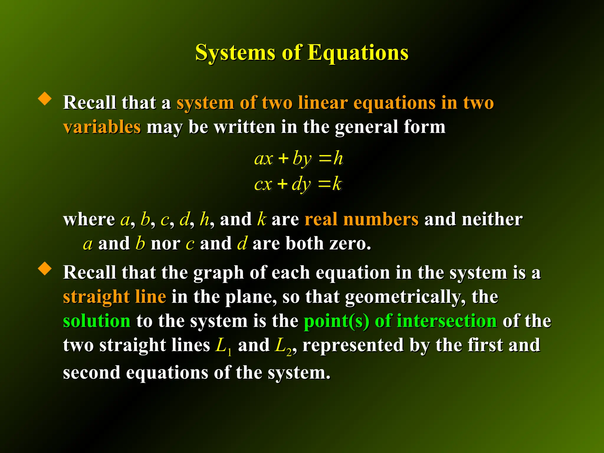
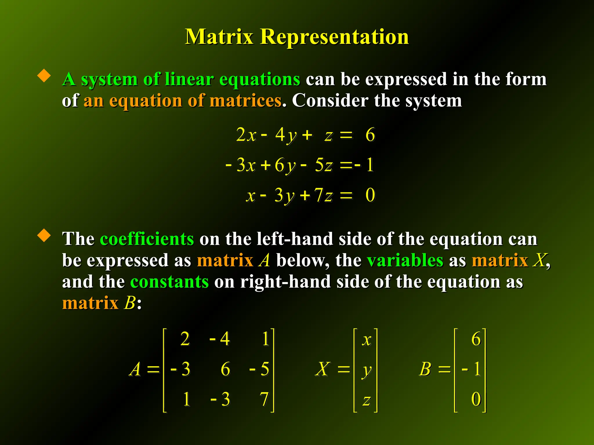
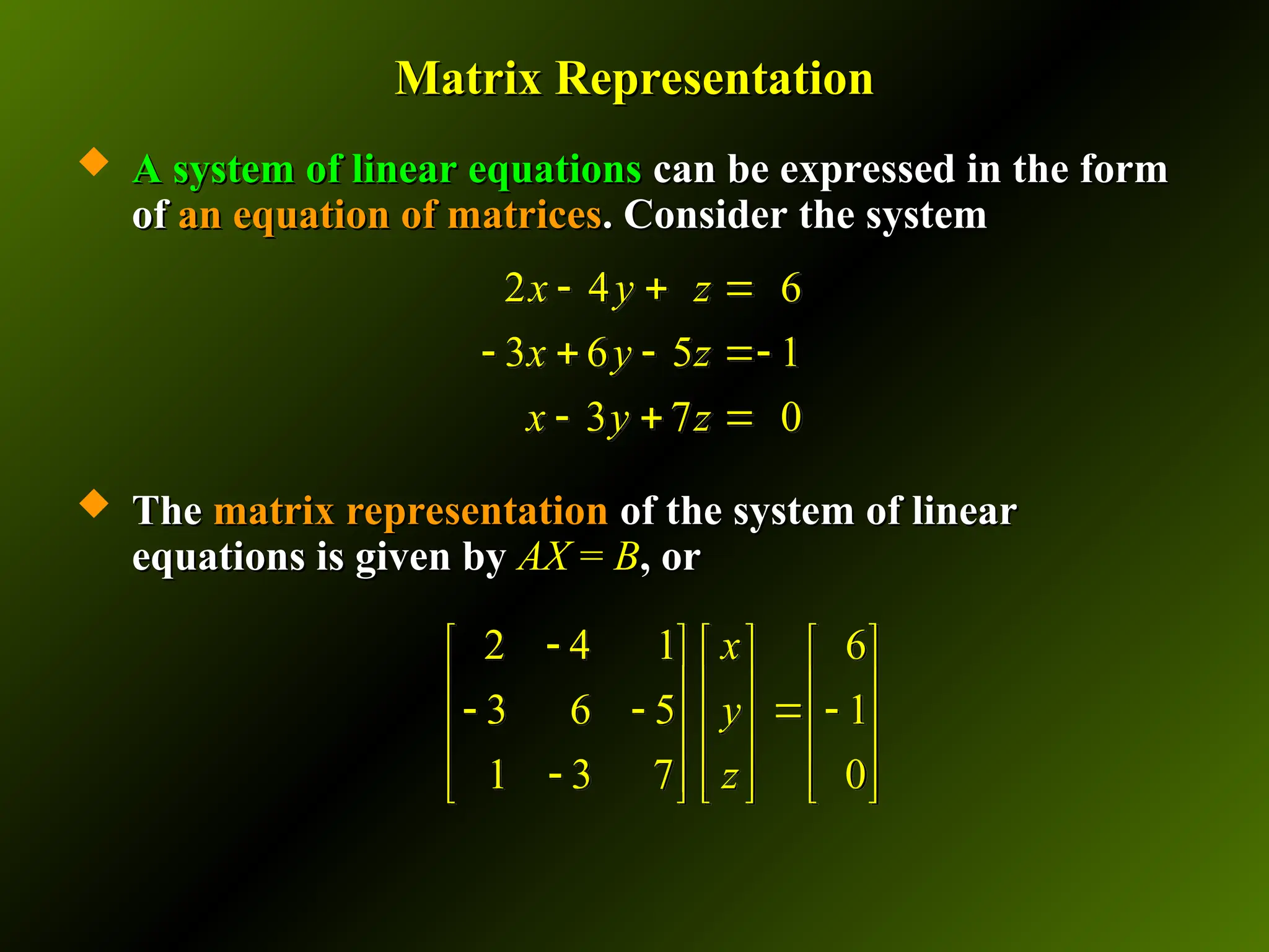
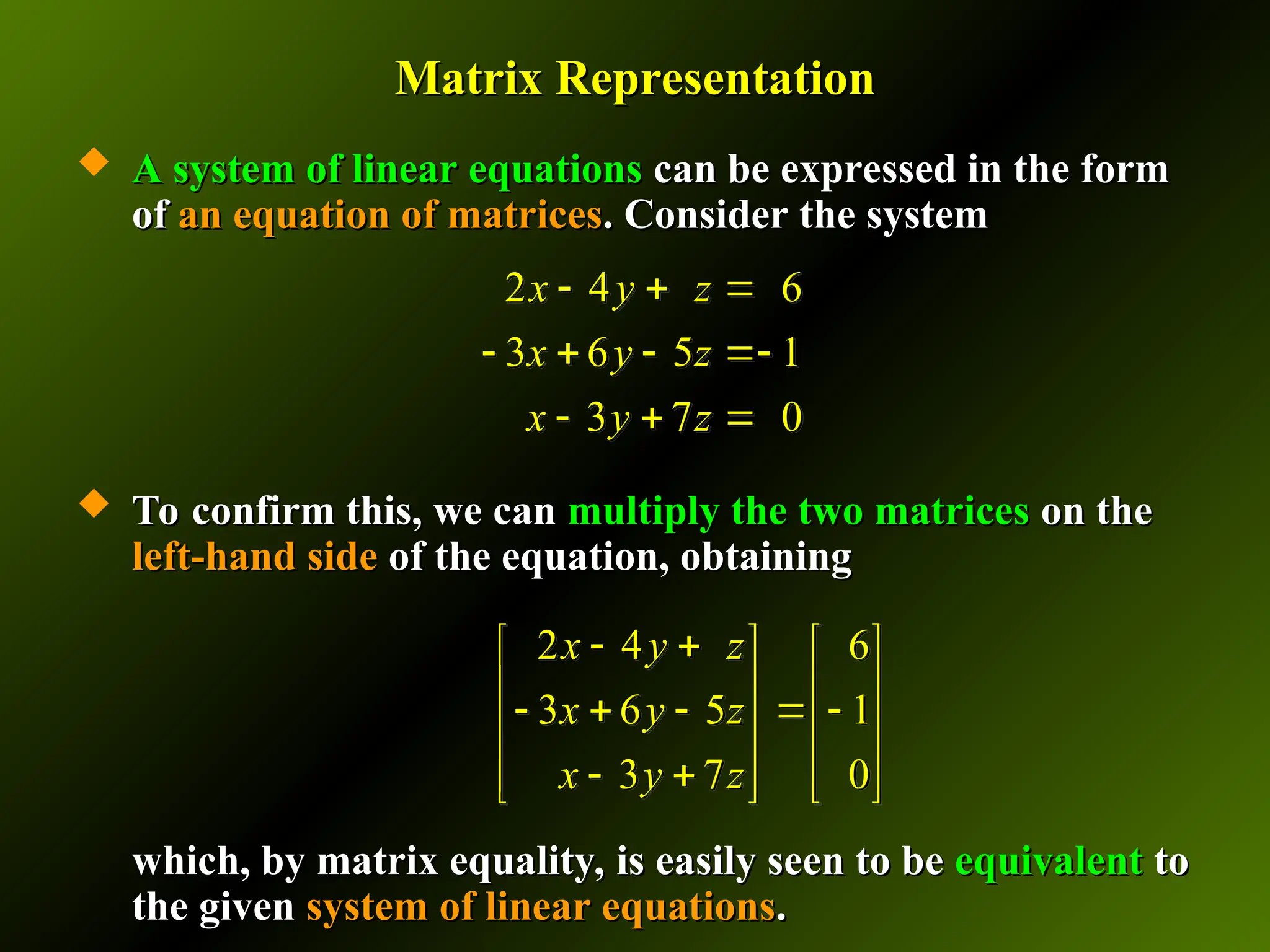
Recall that a system of two linear equations in two variables may be written in the general form
where a, b, c, d, h, and k are real numbers and neither a and b nor c and d are both zero.
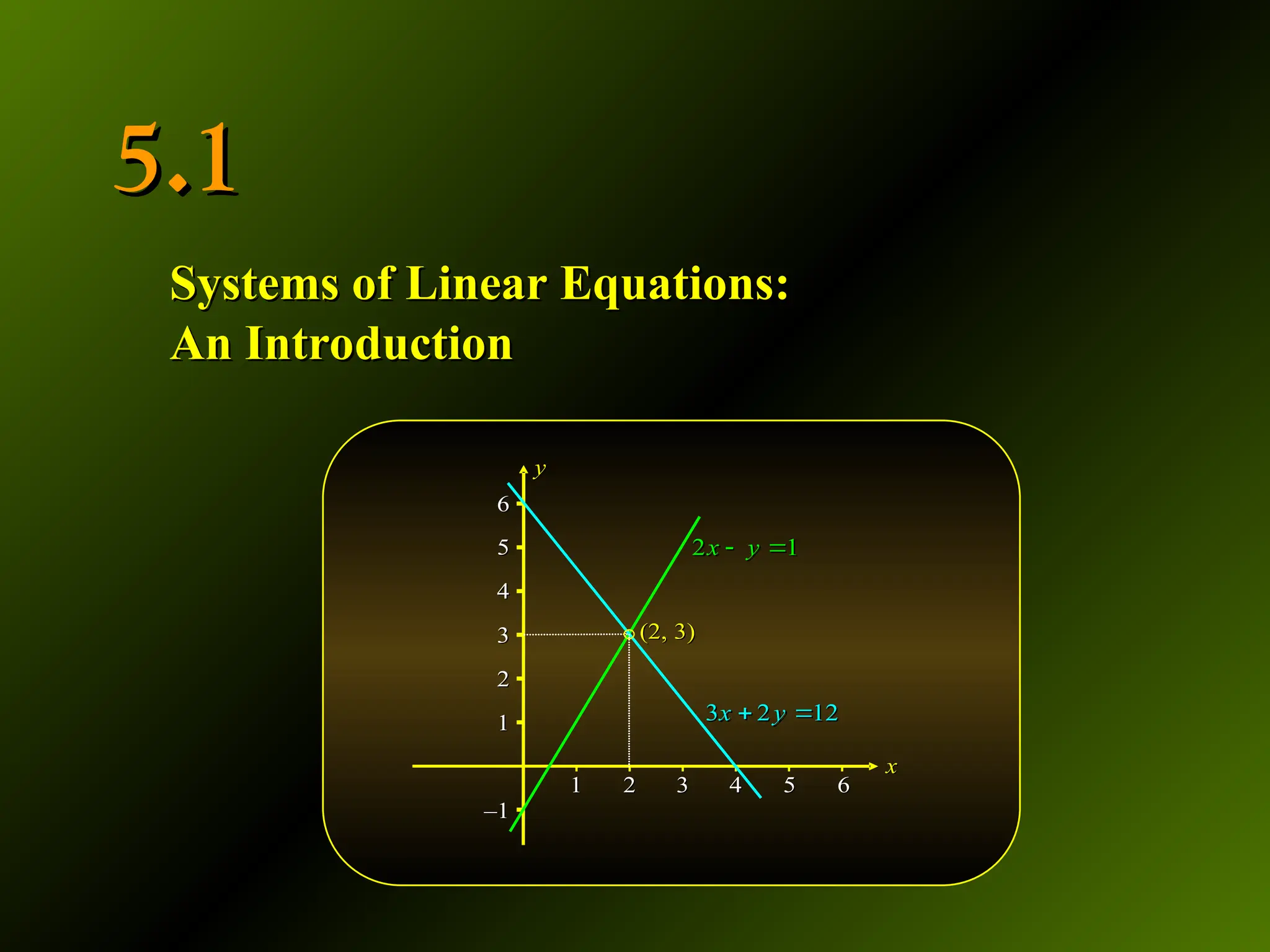
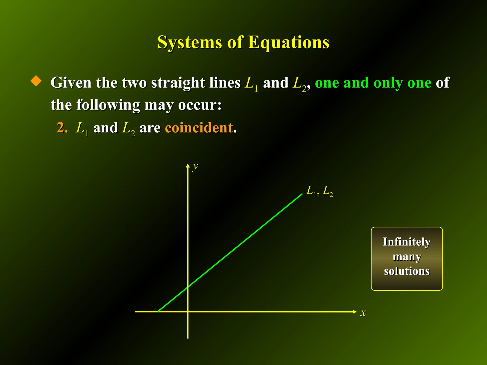
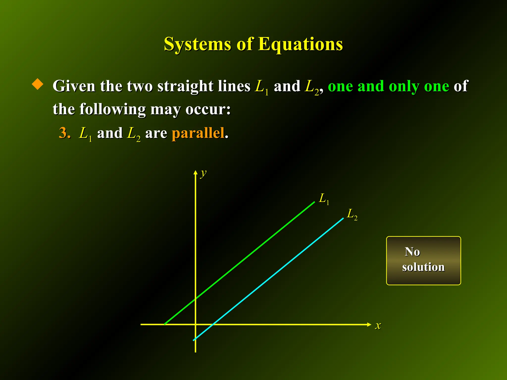
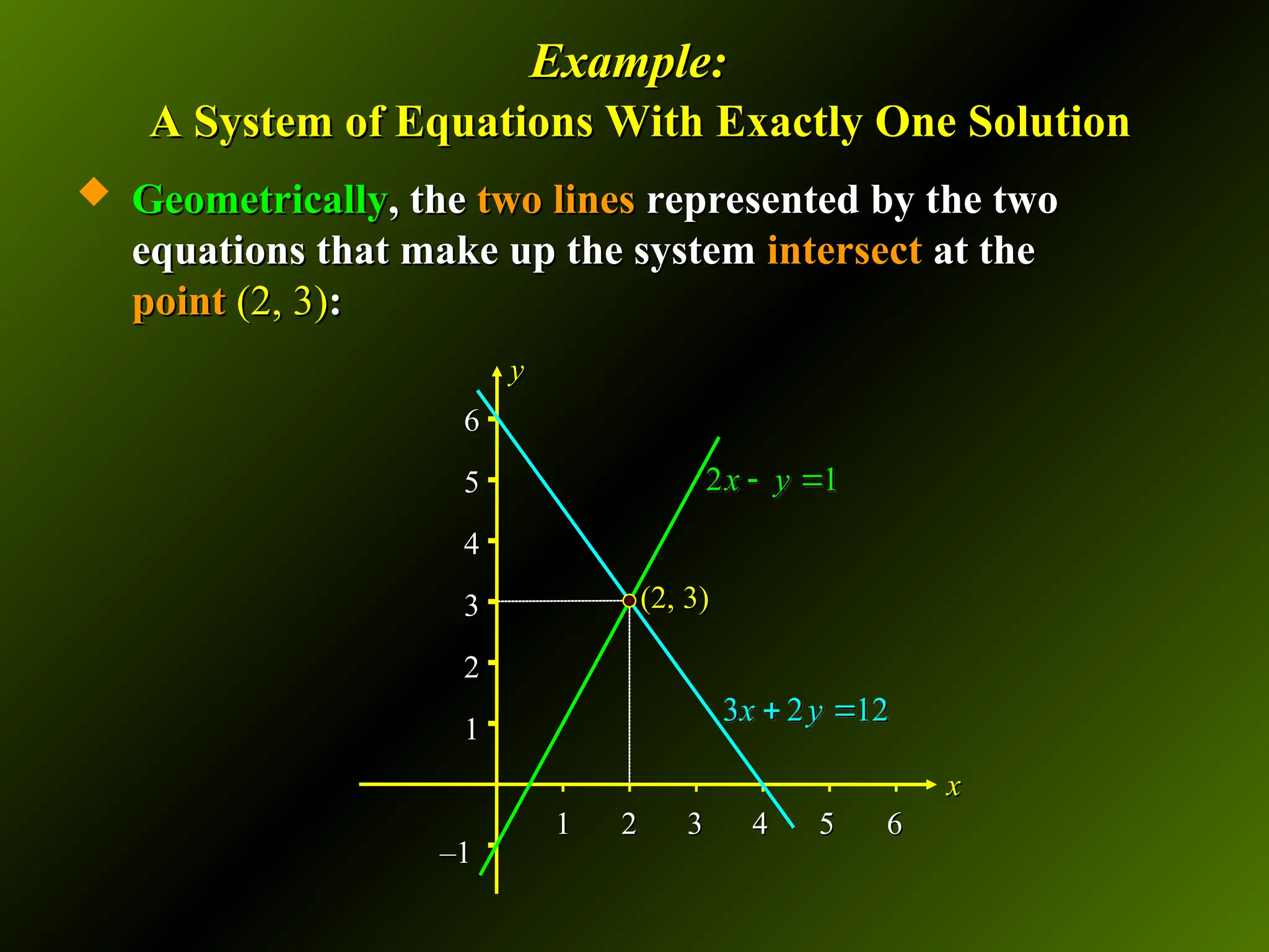
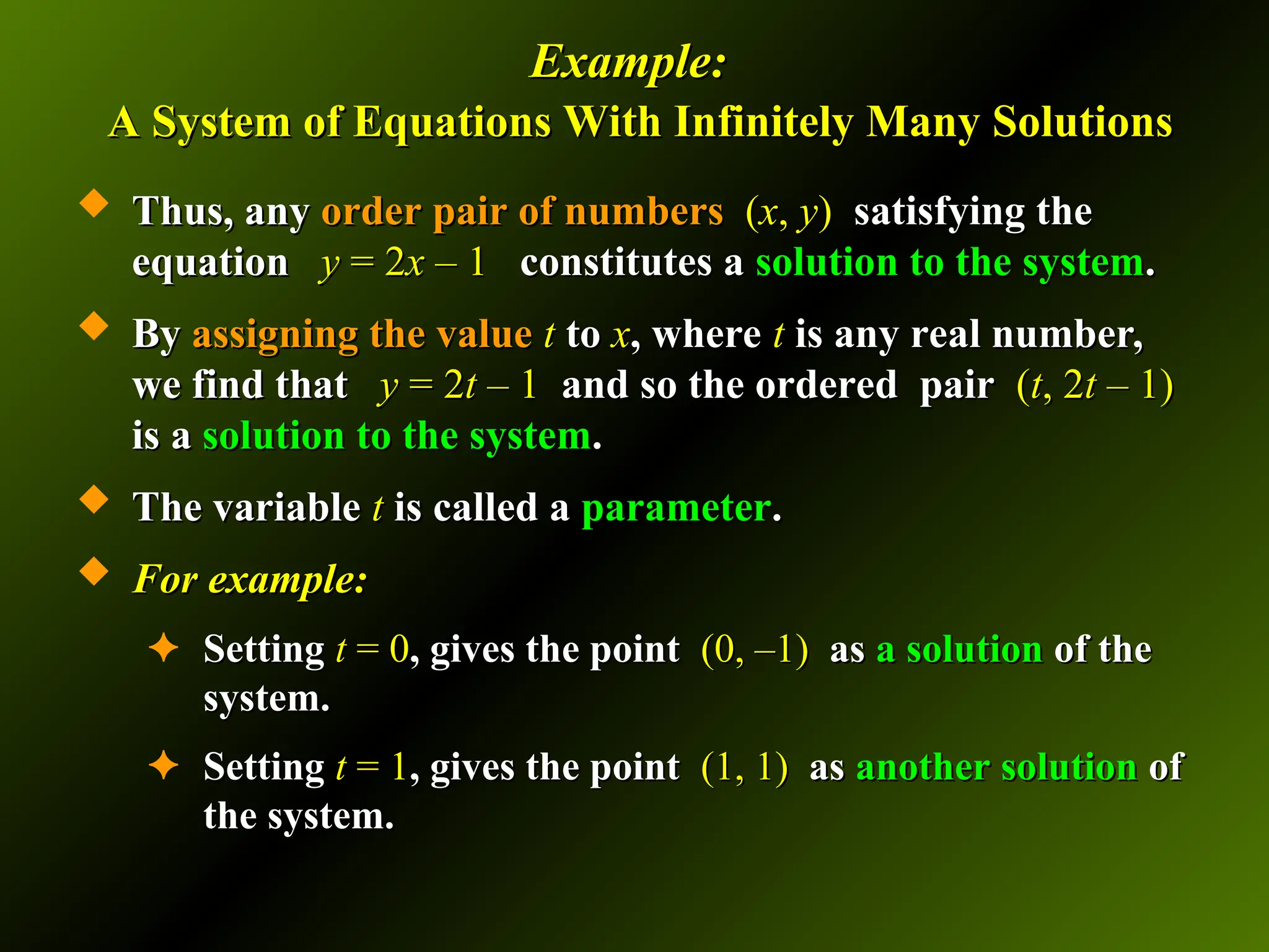
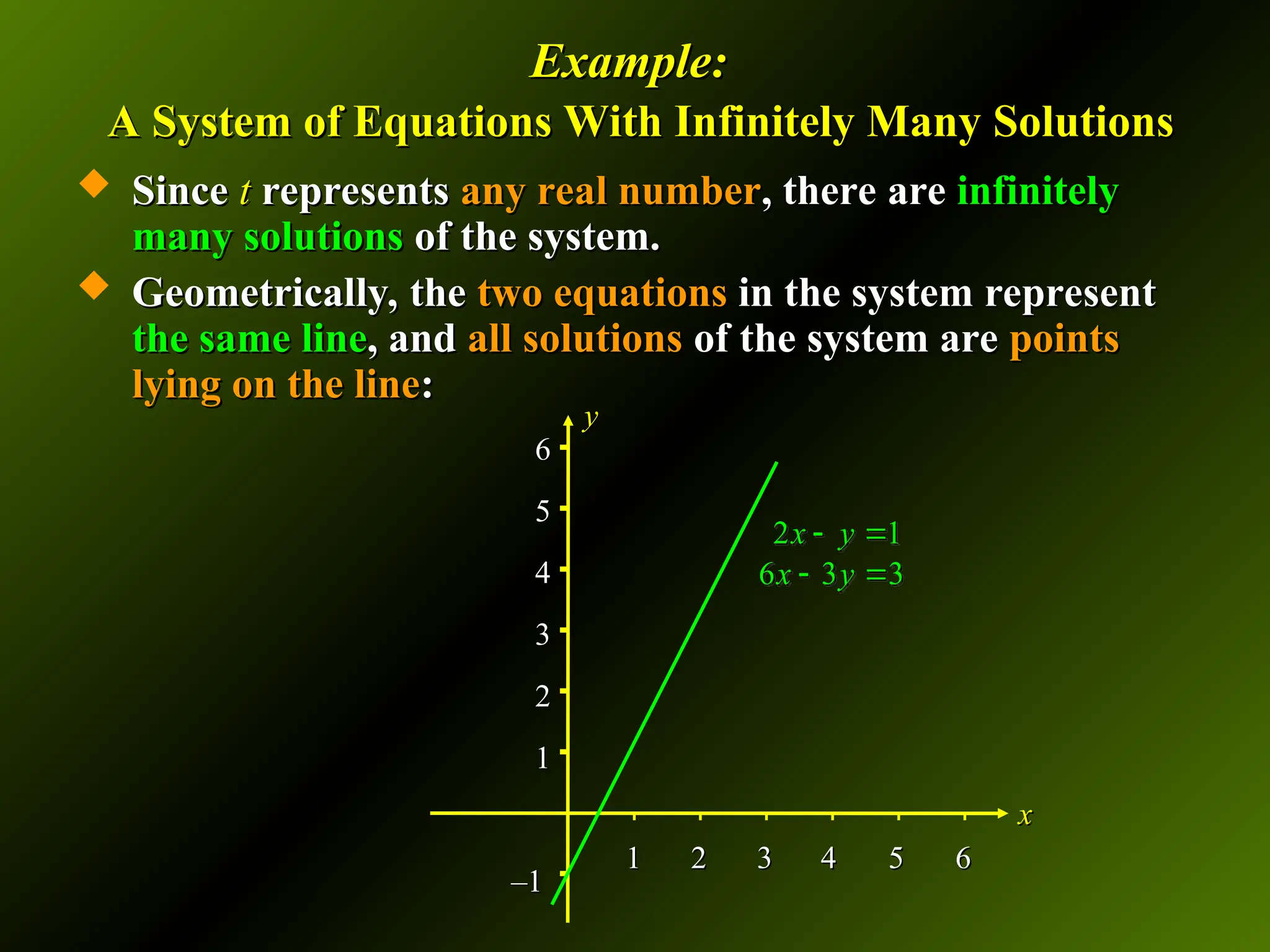
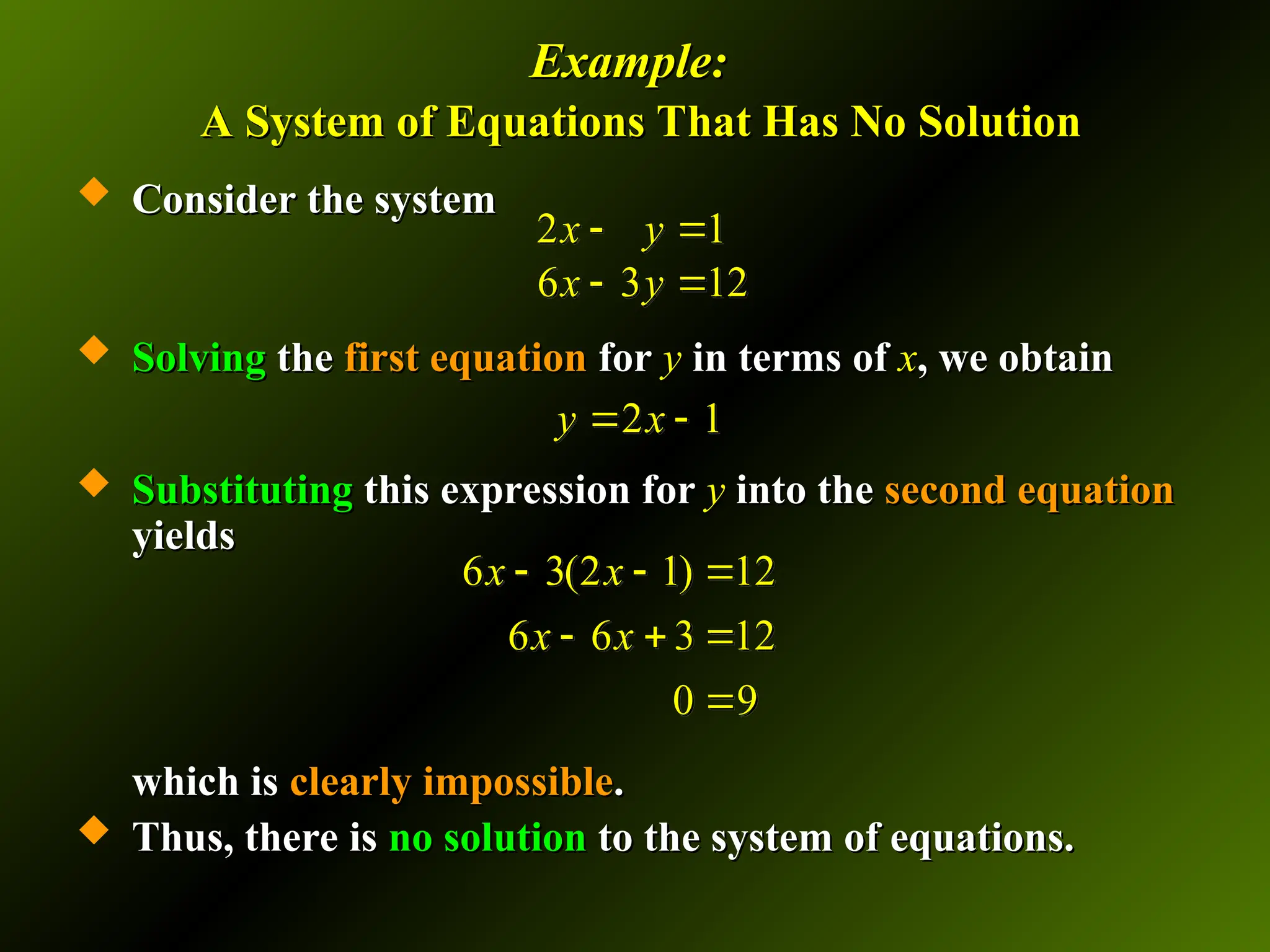
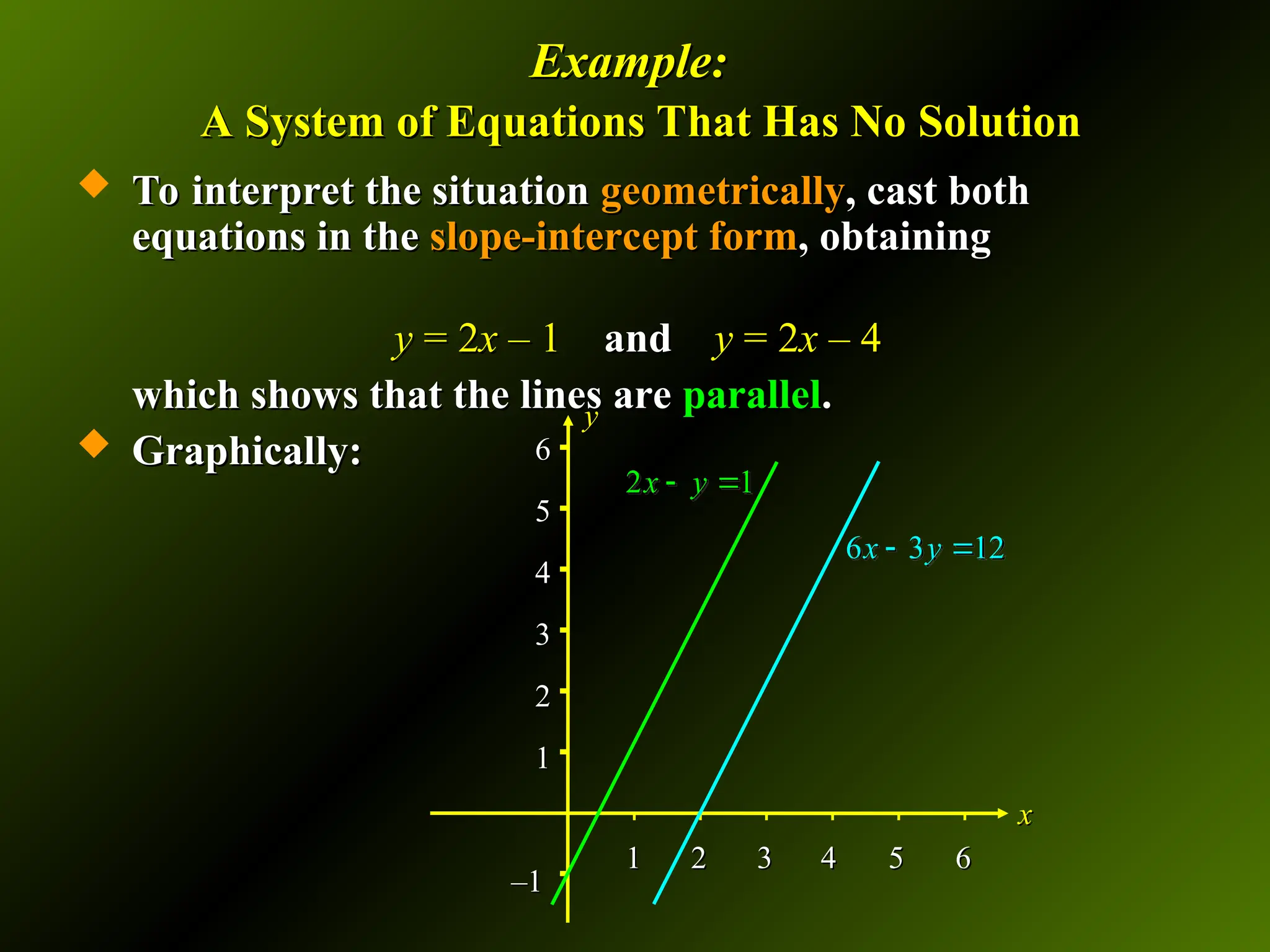
Recall that the graph of each equation in the system is a straight line in the plane, so that geometrically, the solution to the system is the point(s) of intersection of the two straight lines L1 and L2, represented by the first and second equations of the system.Thus, any order pair of numbers (x, y) satisfying the equation y = 2x – 1 constitutes a solution to the system.
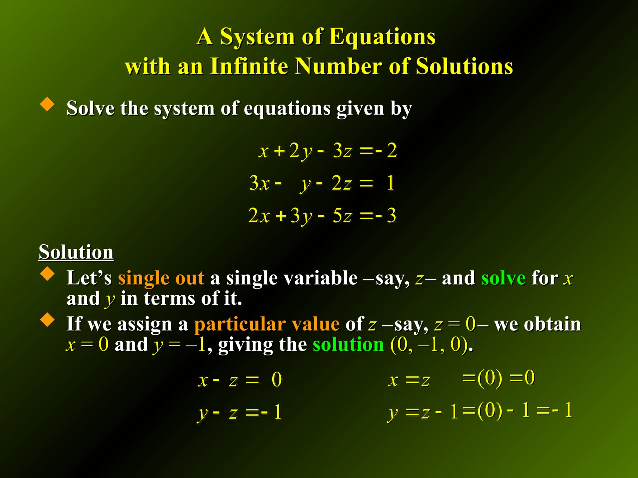
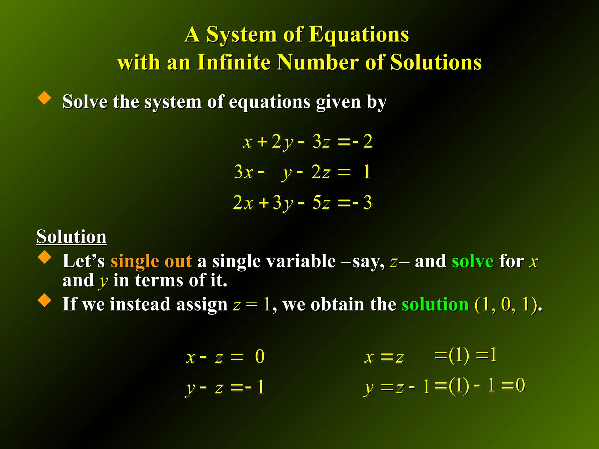
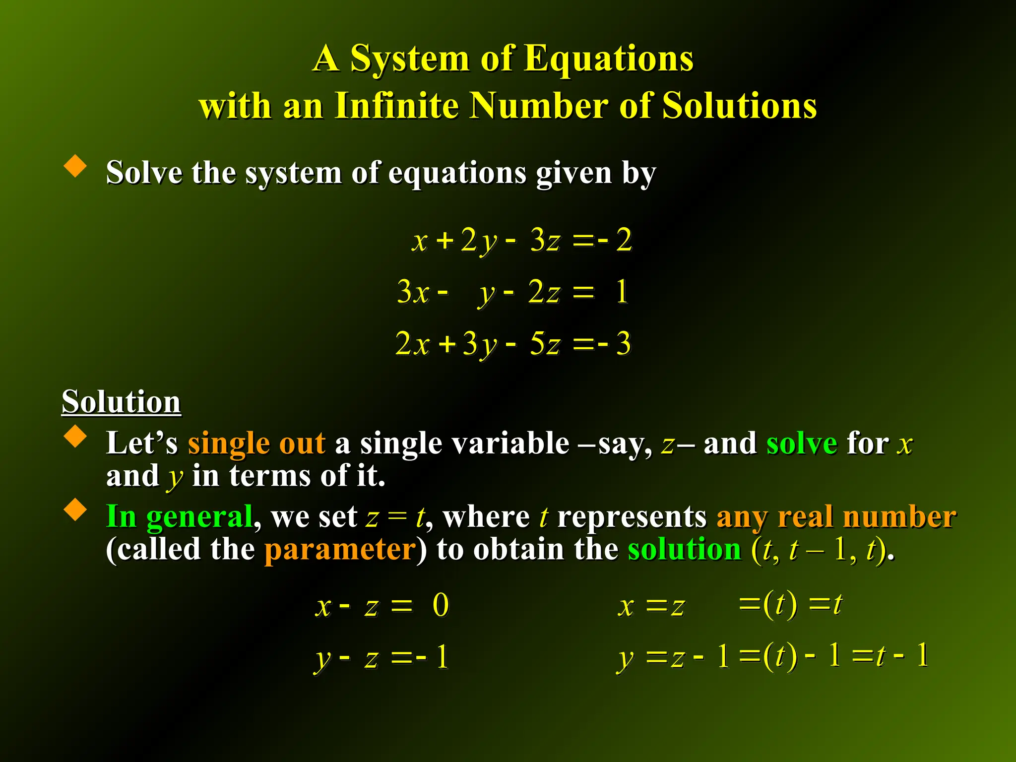
By assigning the value t to x, where t is any real number, we find that y = 2t – 1 and so the ordered pair (t, 2t – 1) is a solution to the system.
The variable t is called a parameter.
For example:
Setting t = 0, gives the point (0, –1) as a solution of the system.
Setting t = 1, gives the point (1, 1) as another solution of the system.
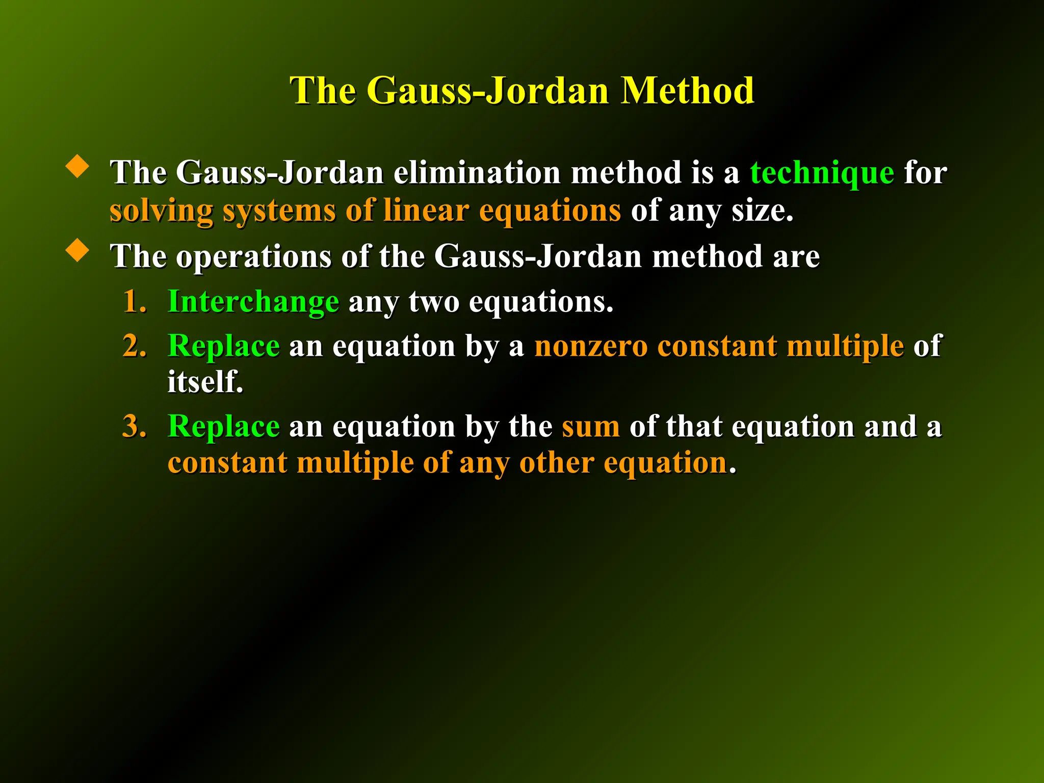
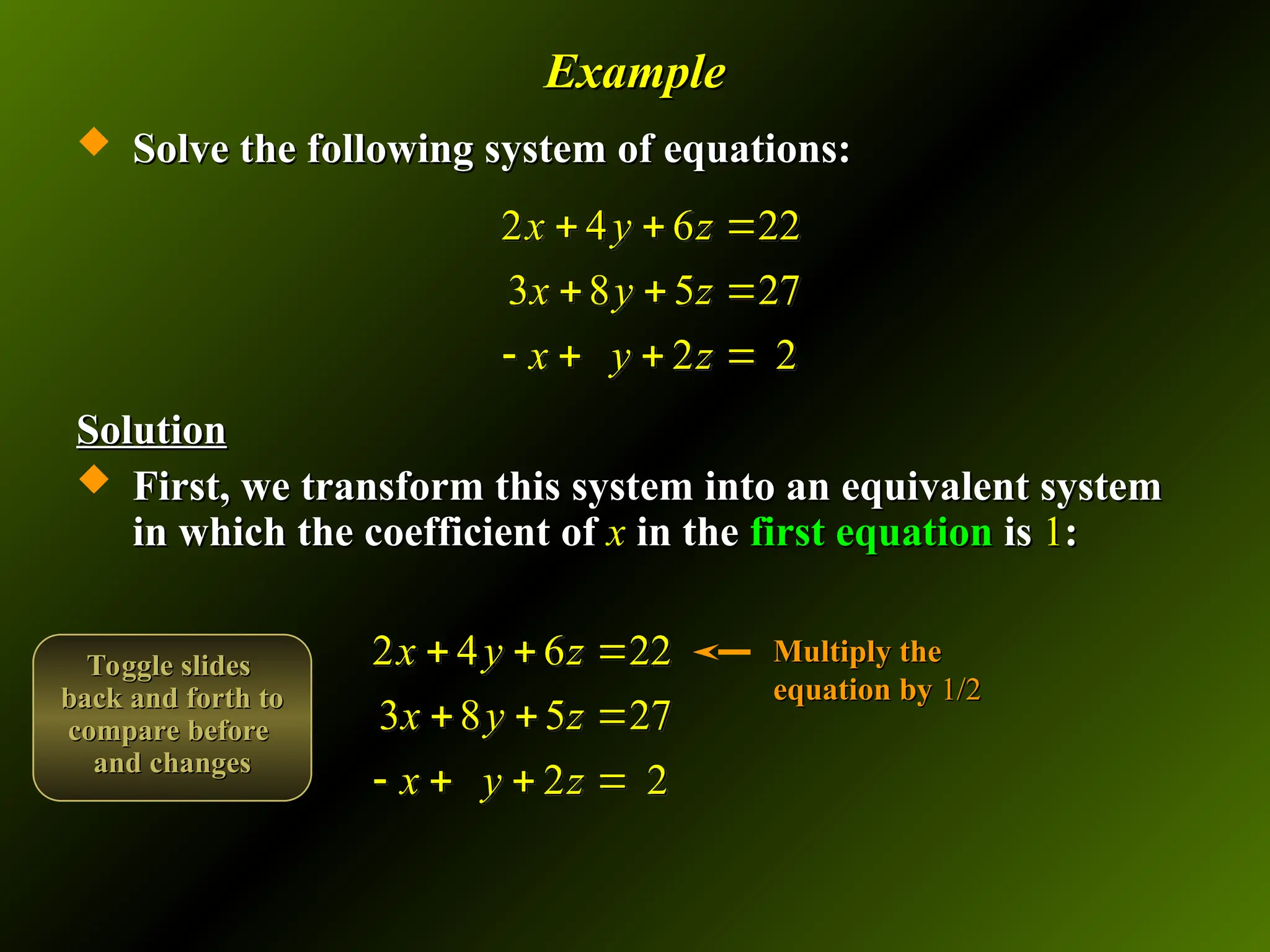
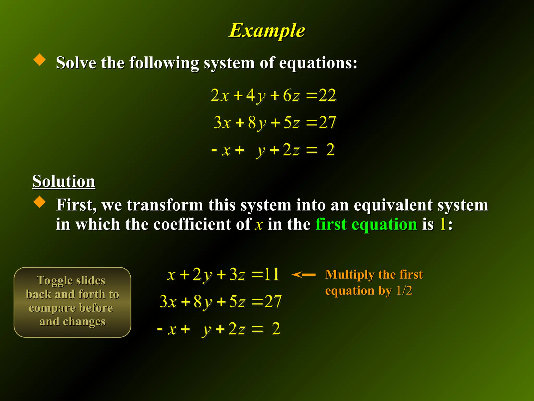
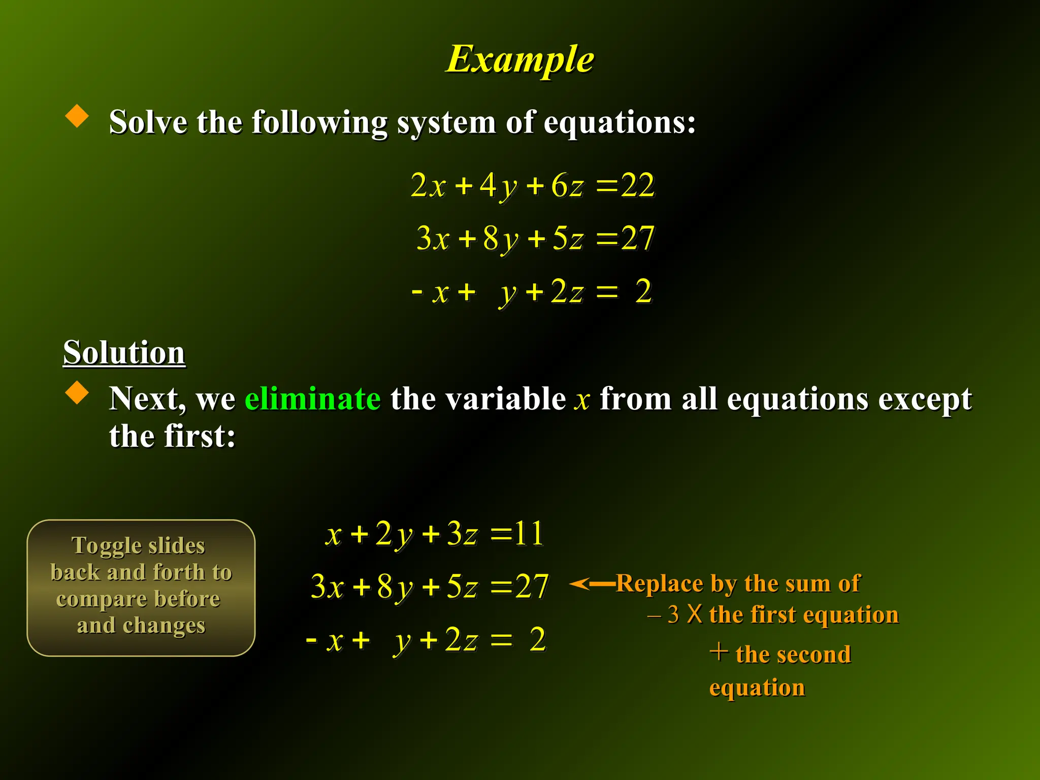
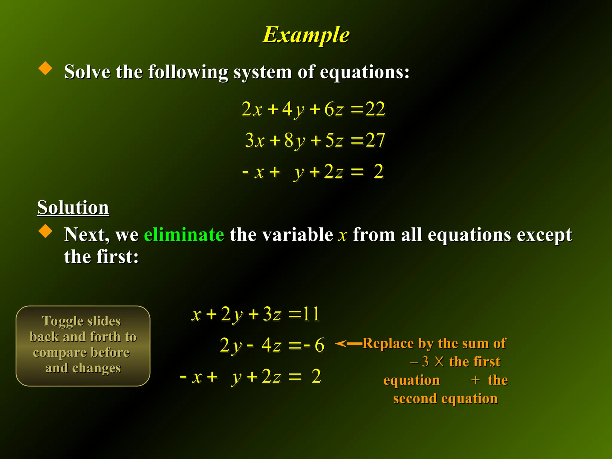
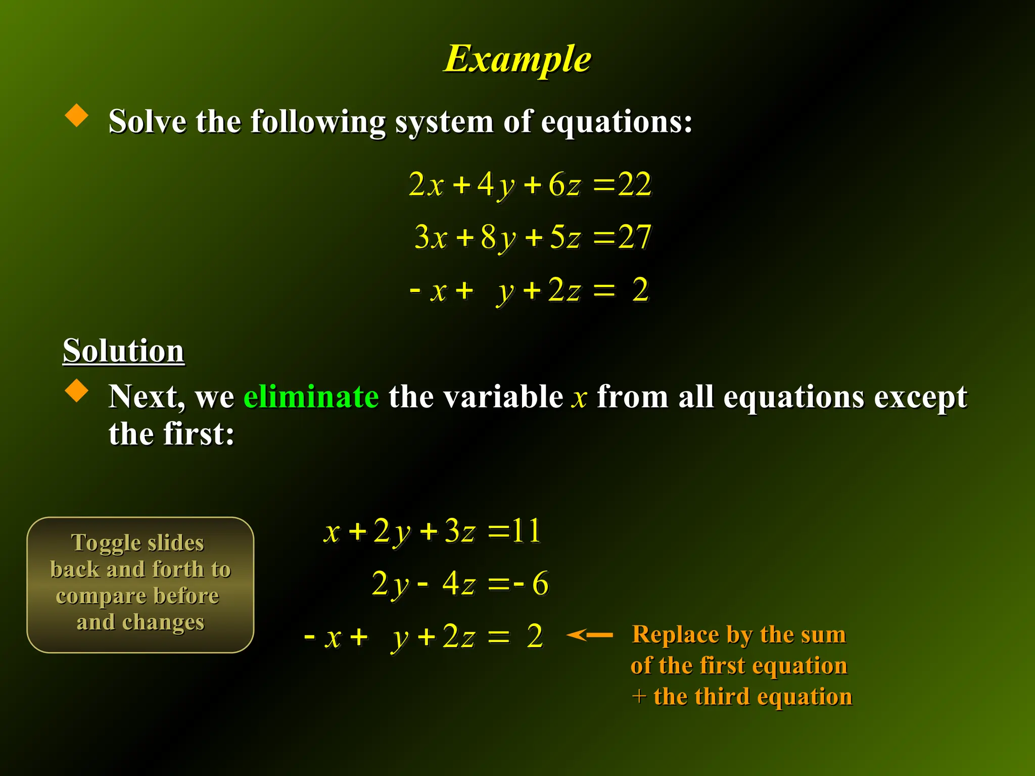
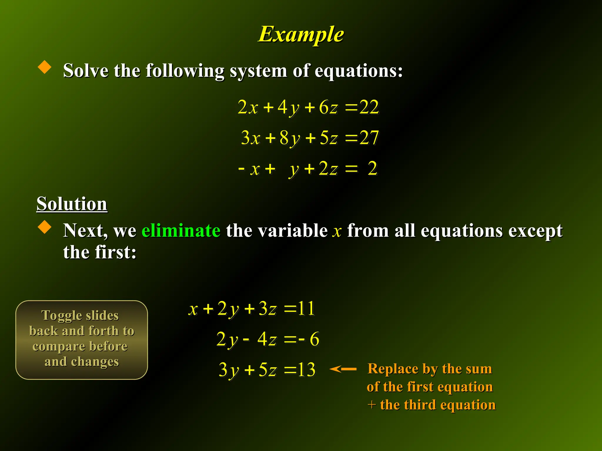
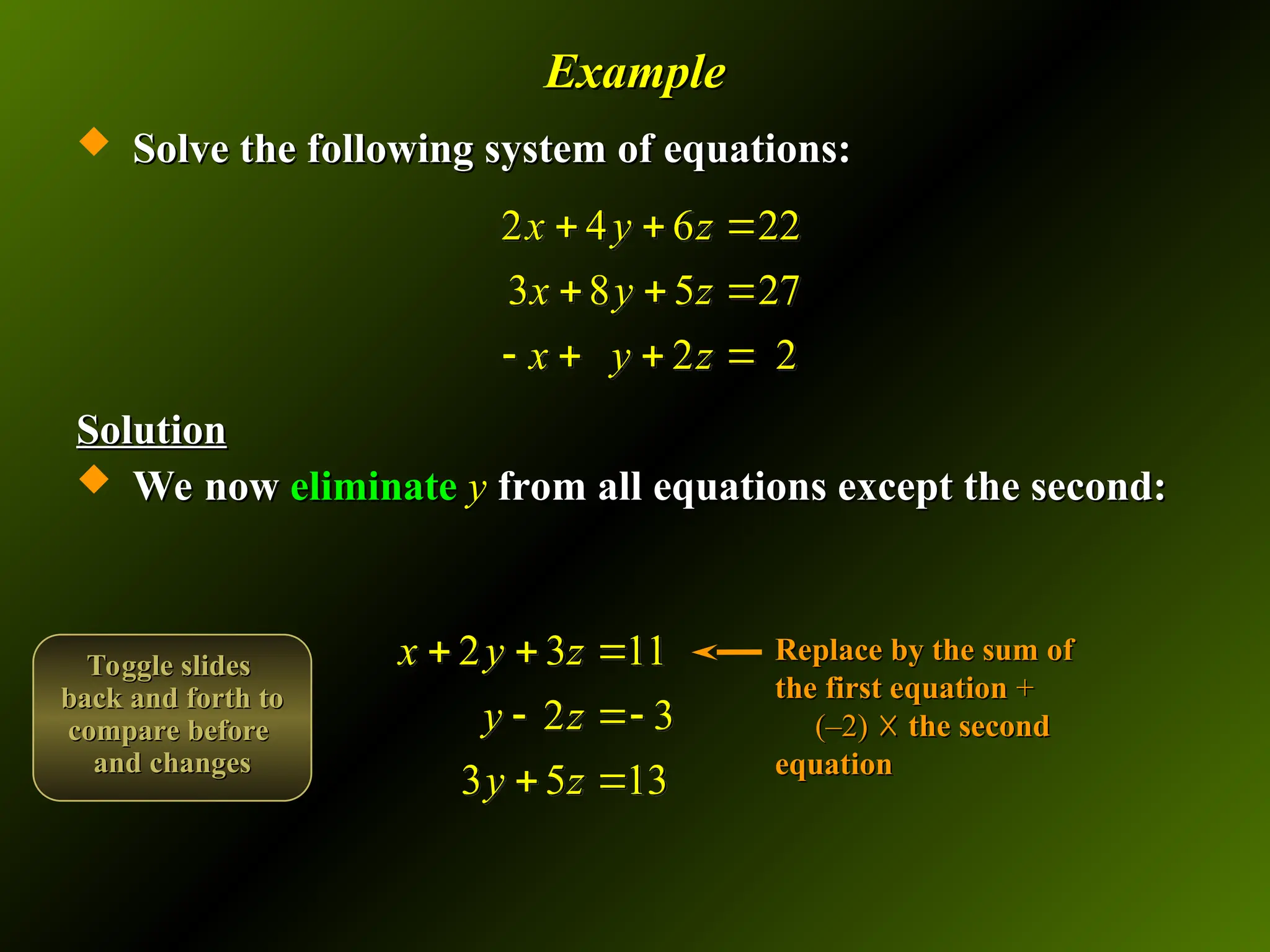
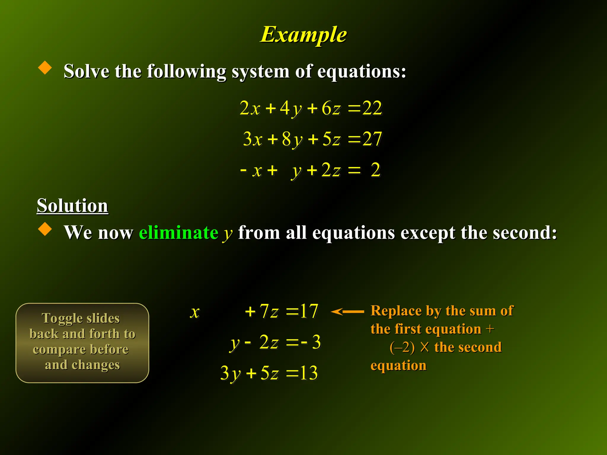
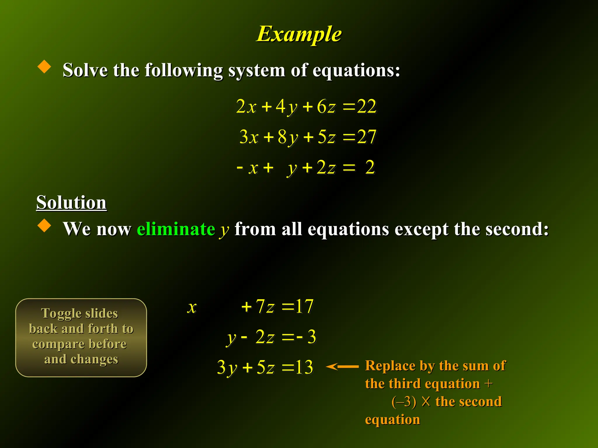
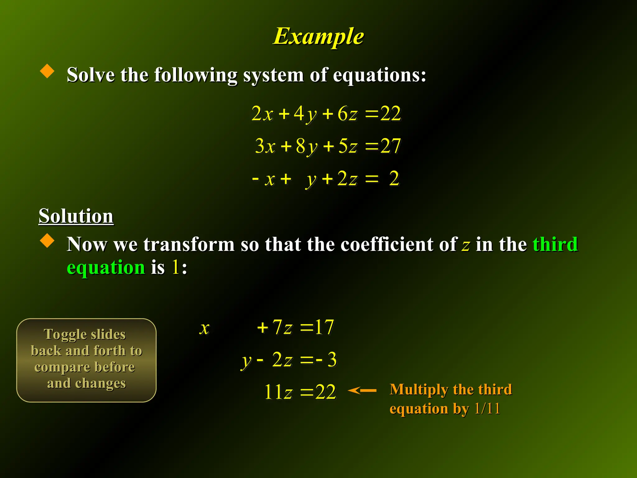
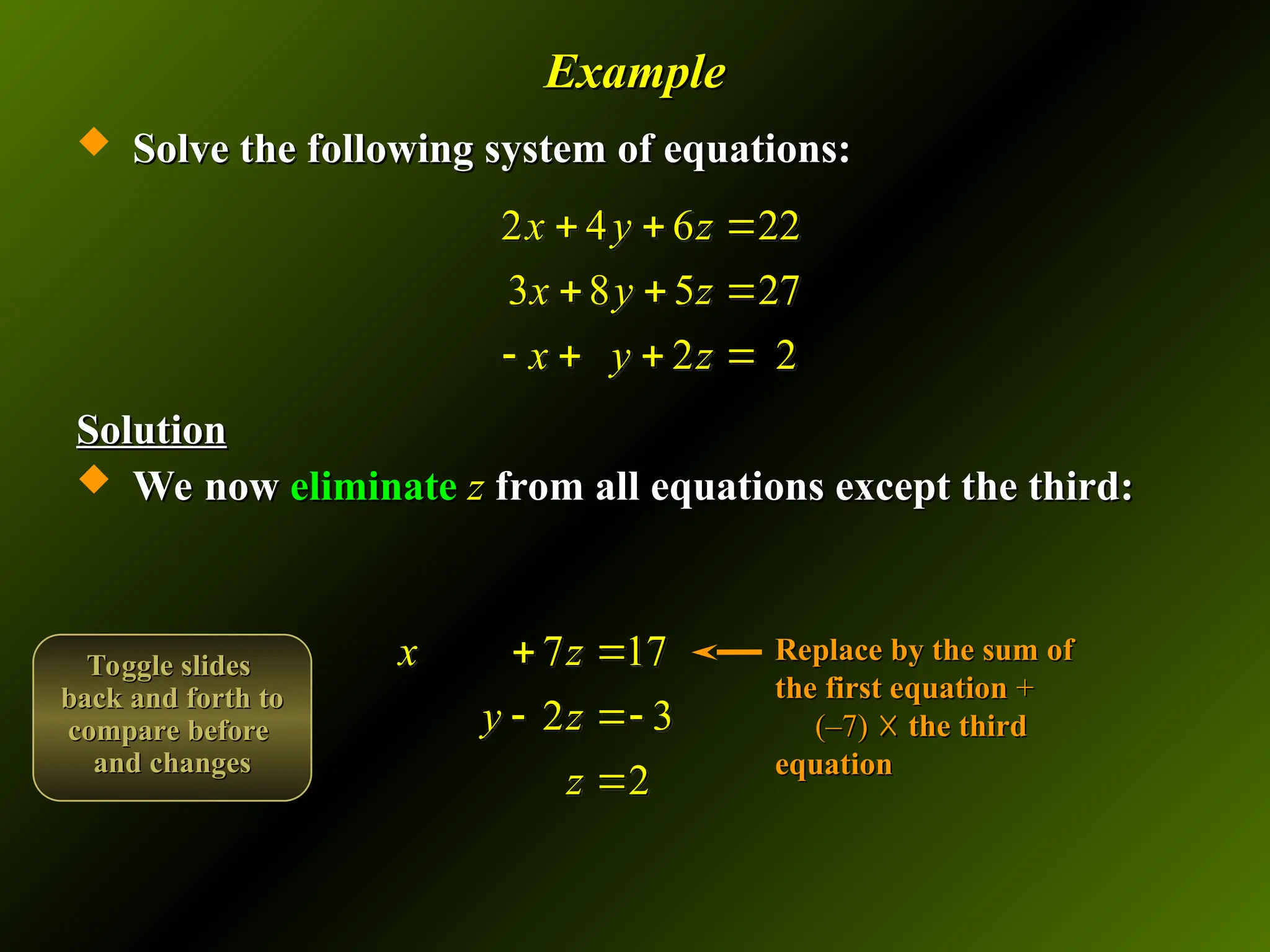
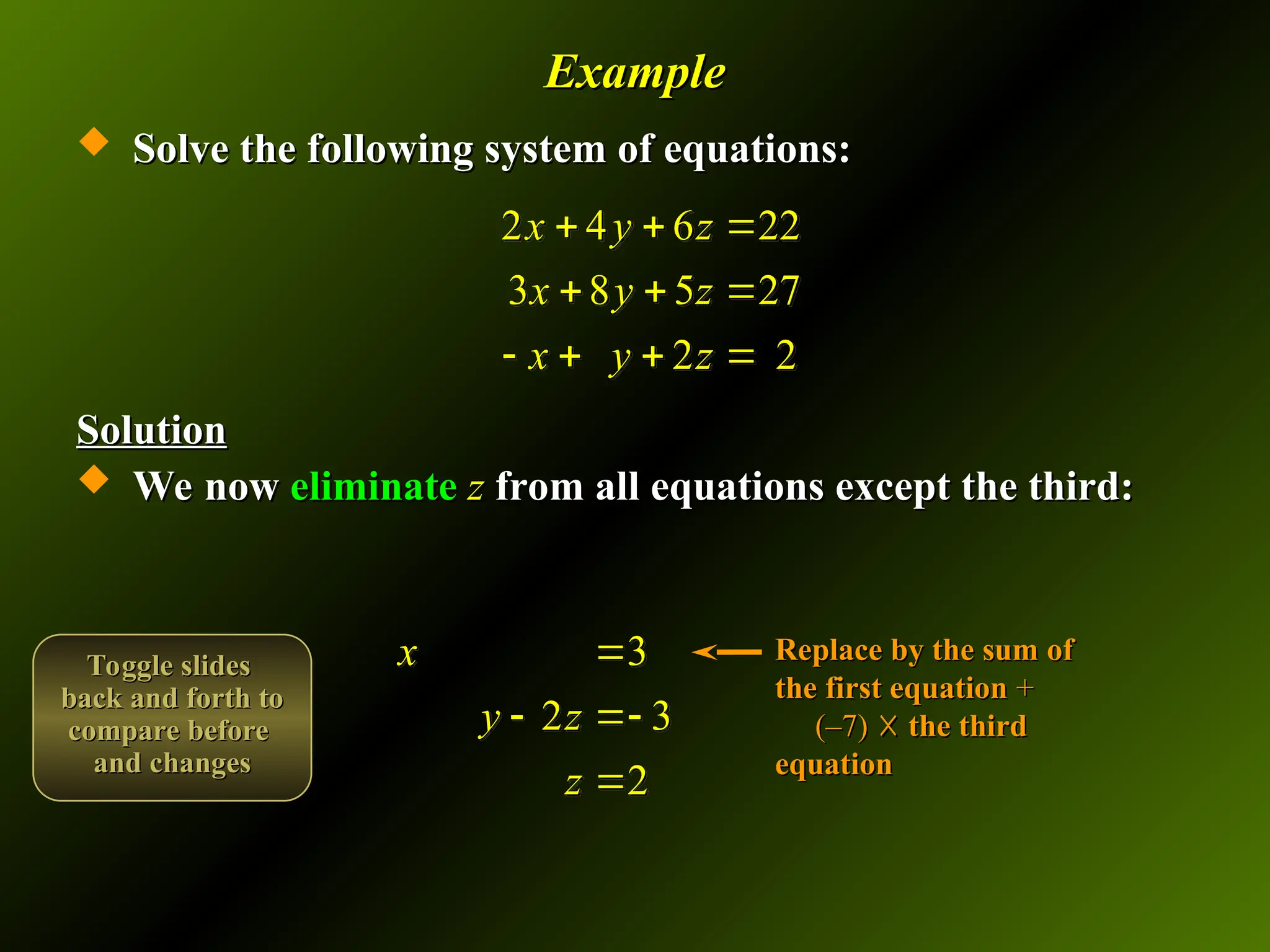
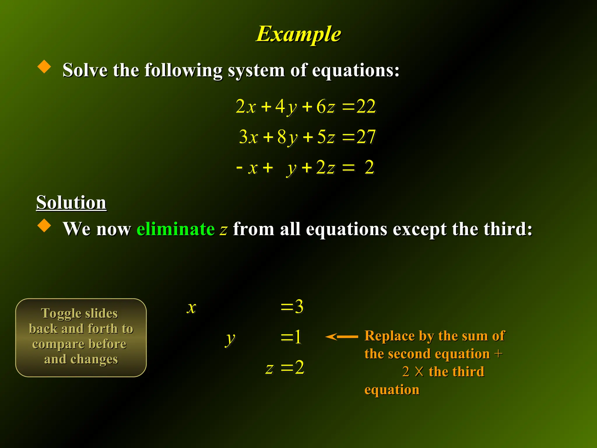
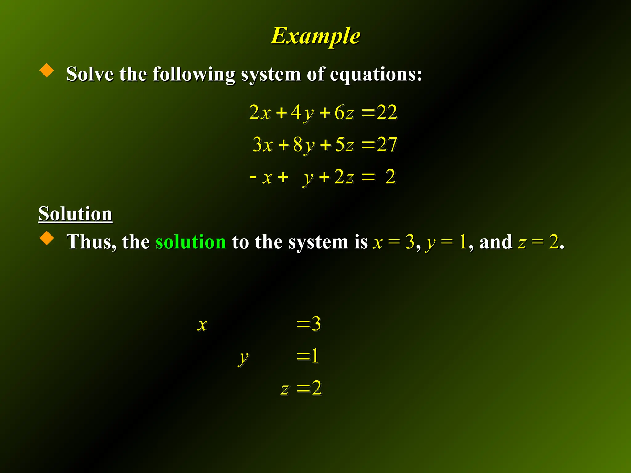
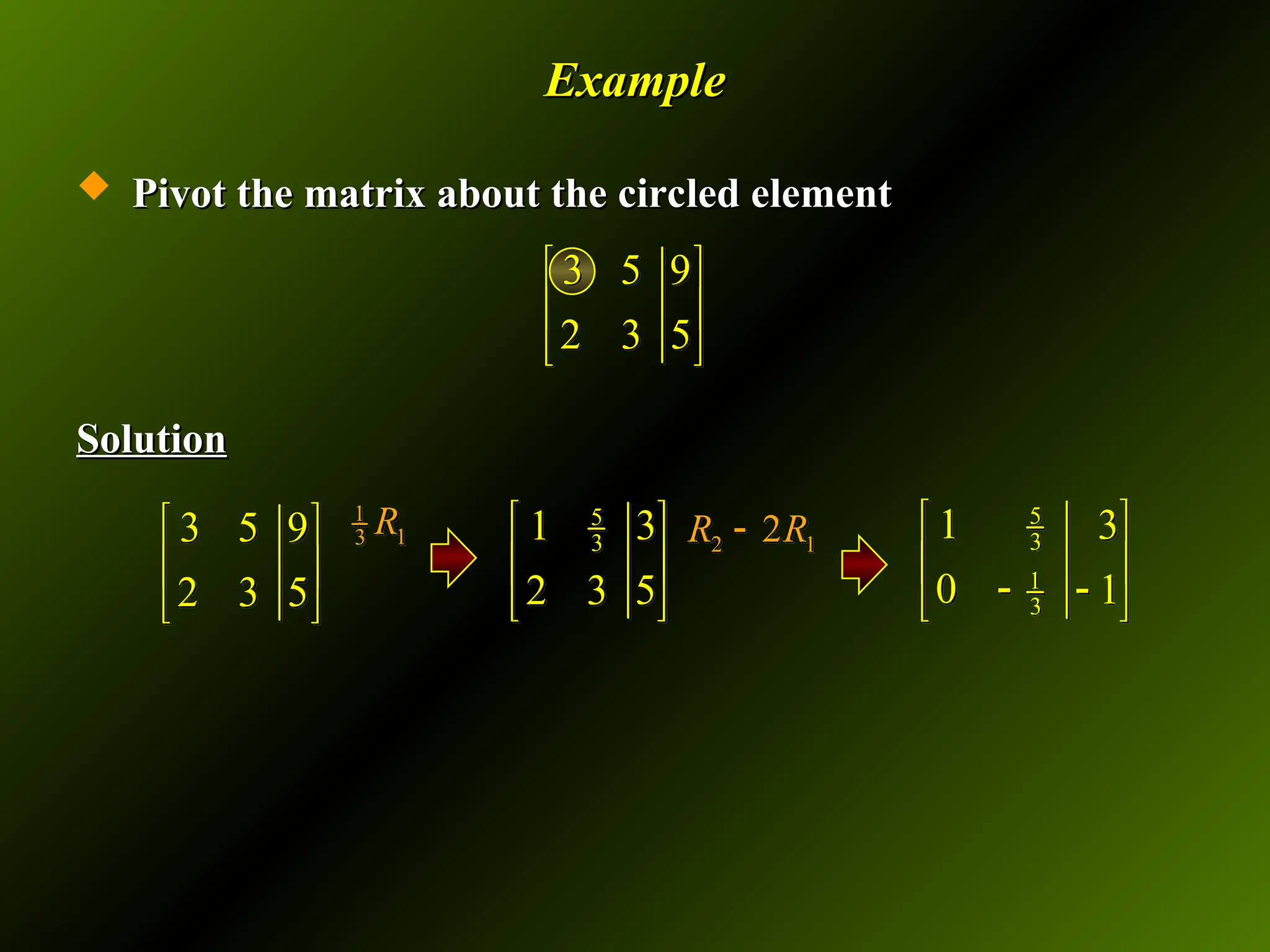
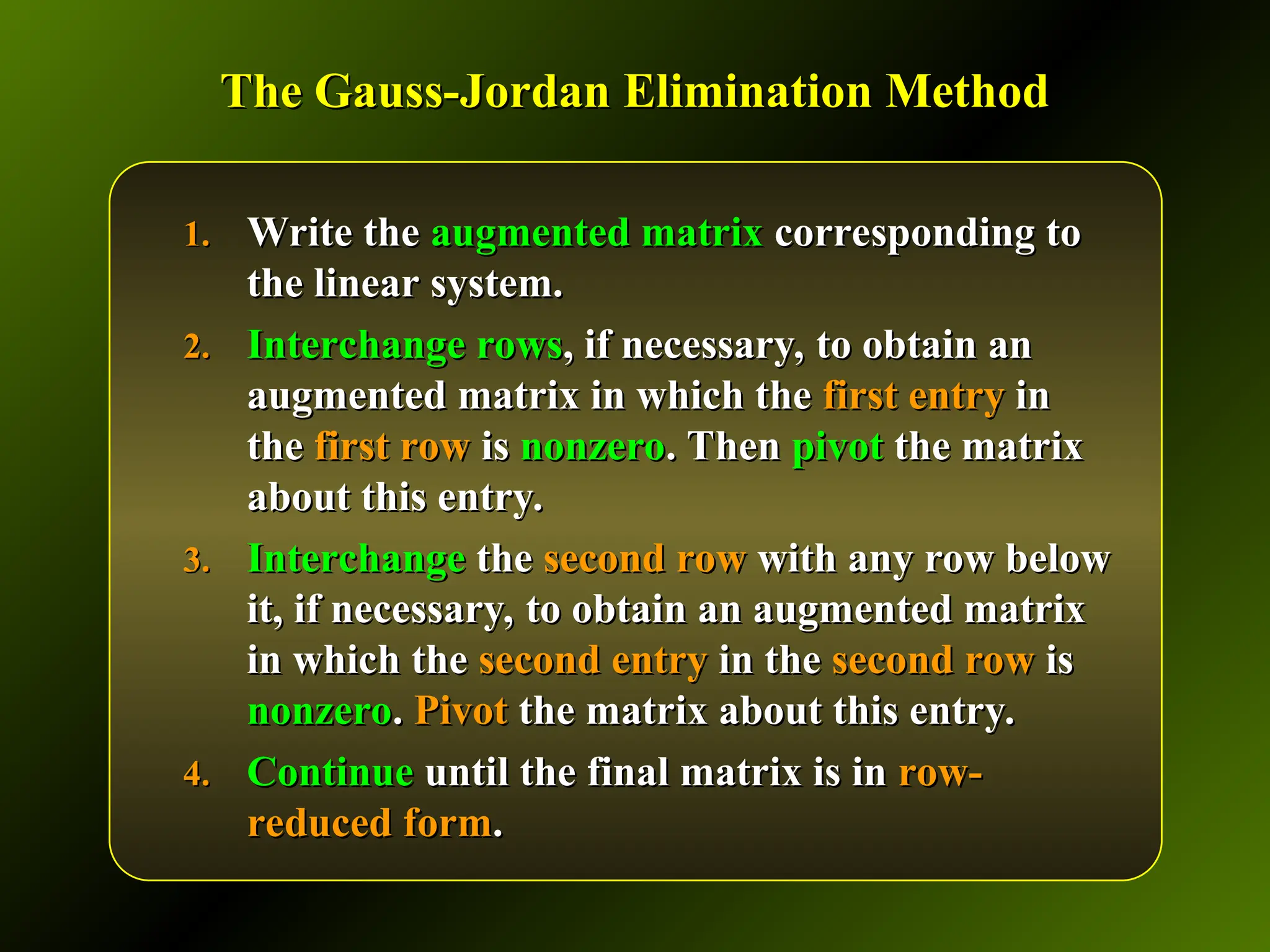
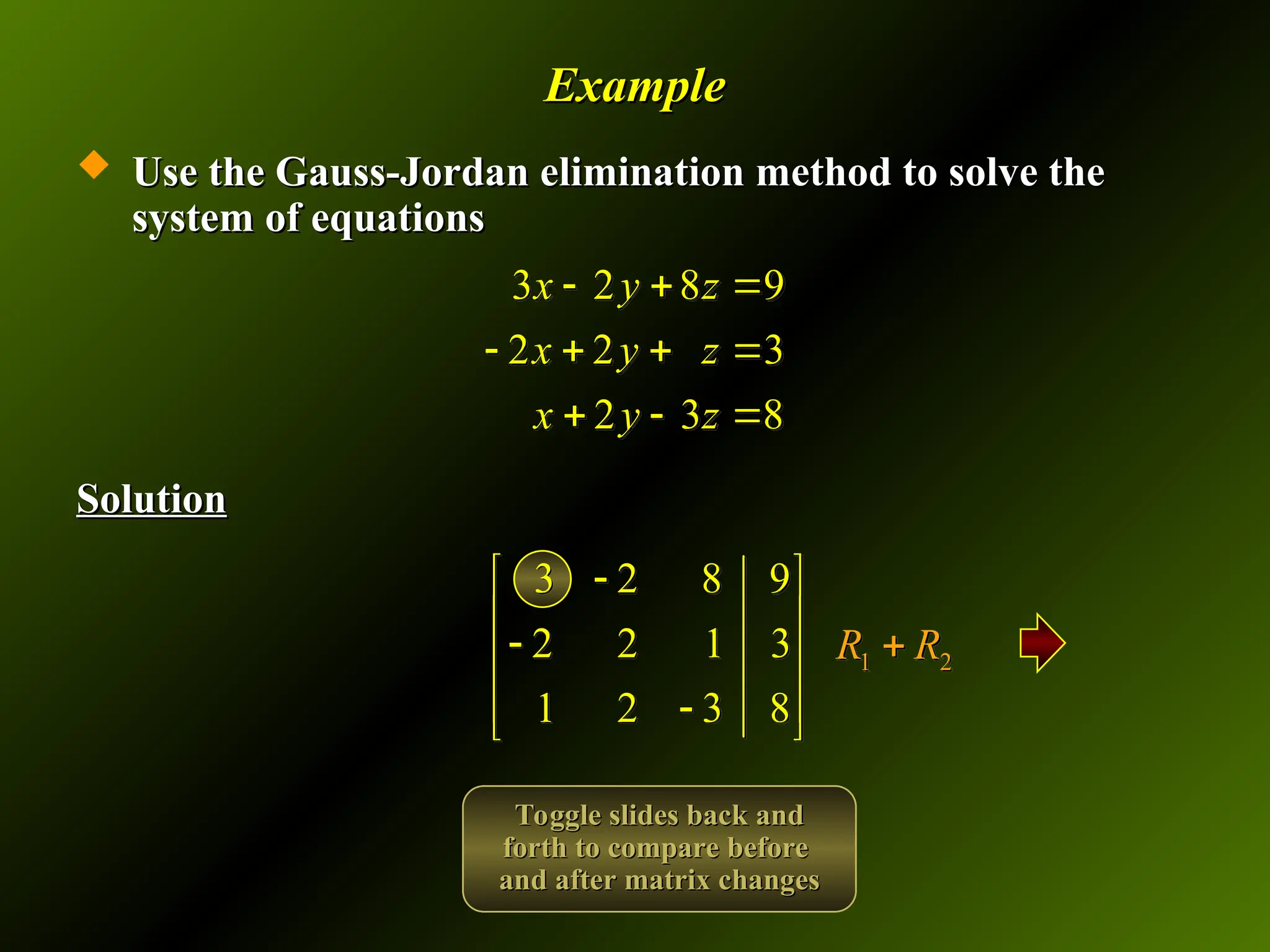
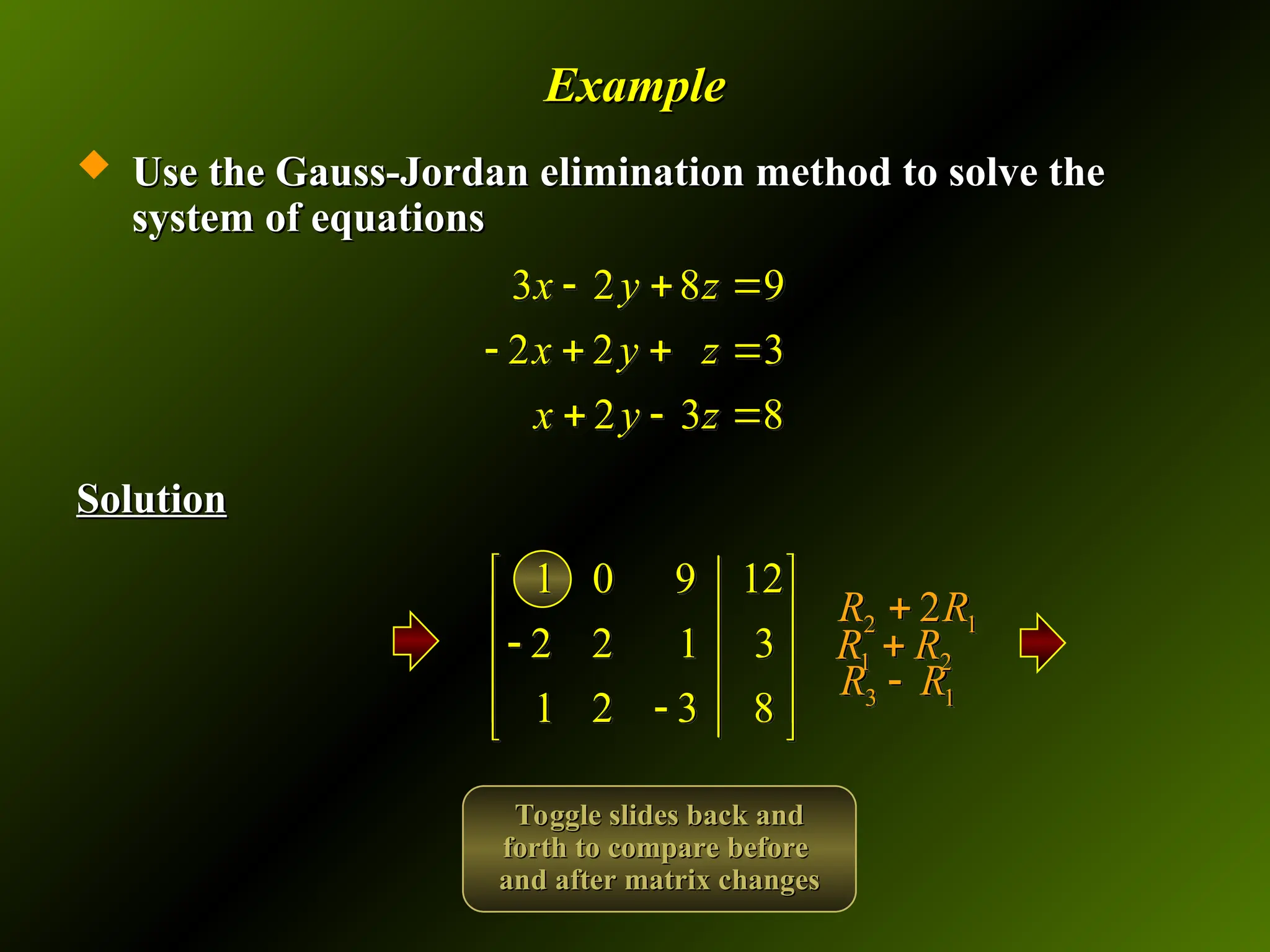
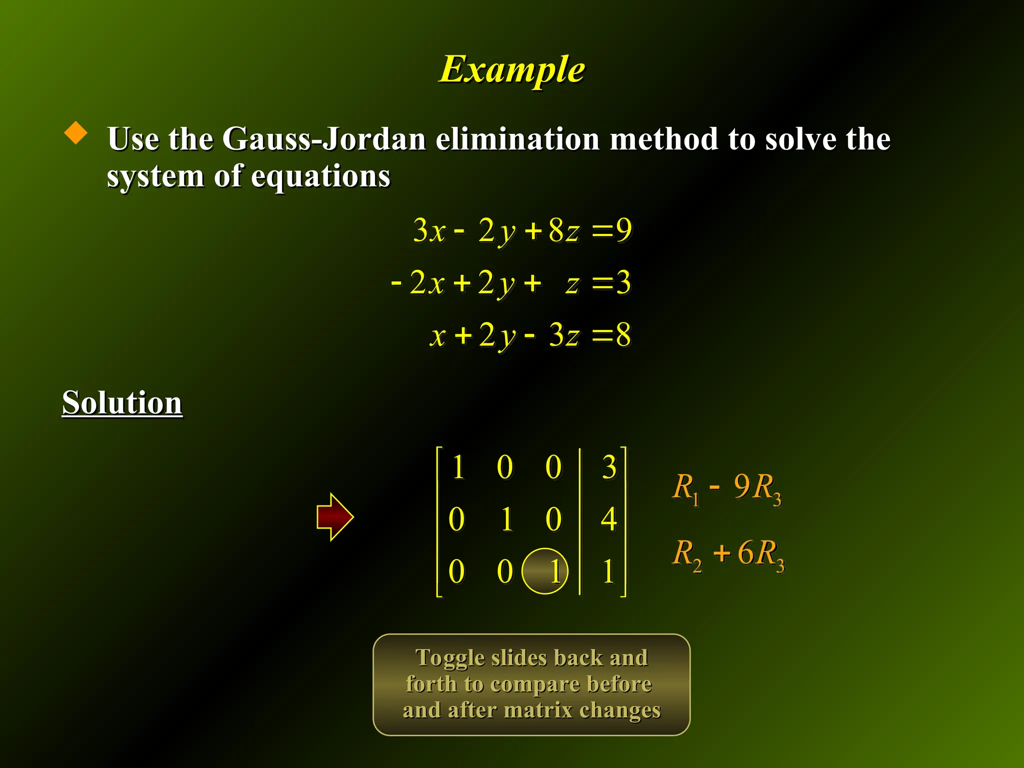
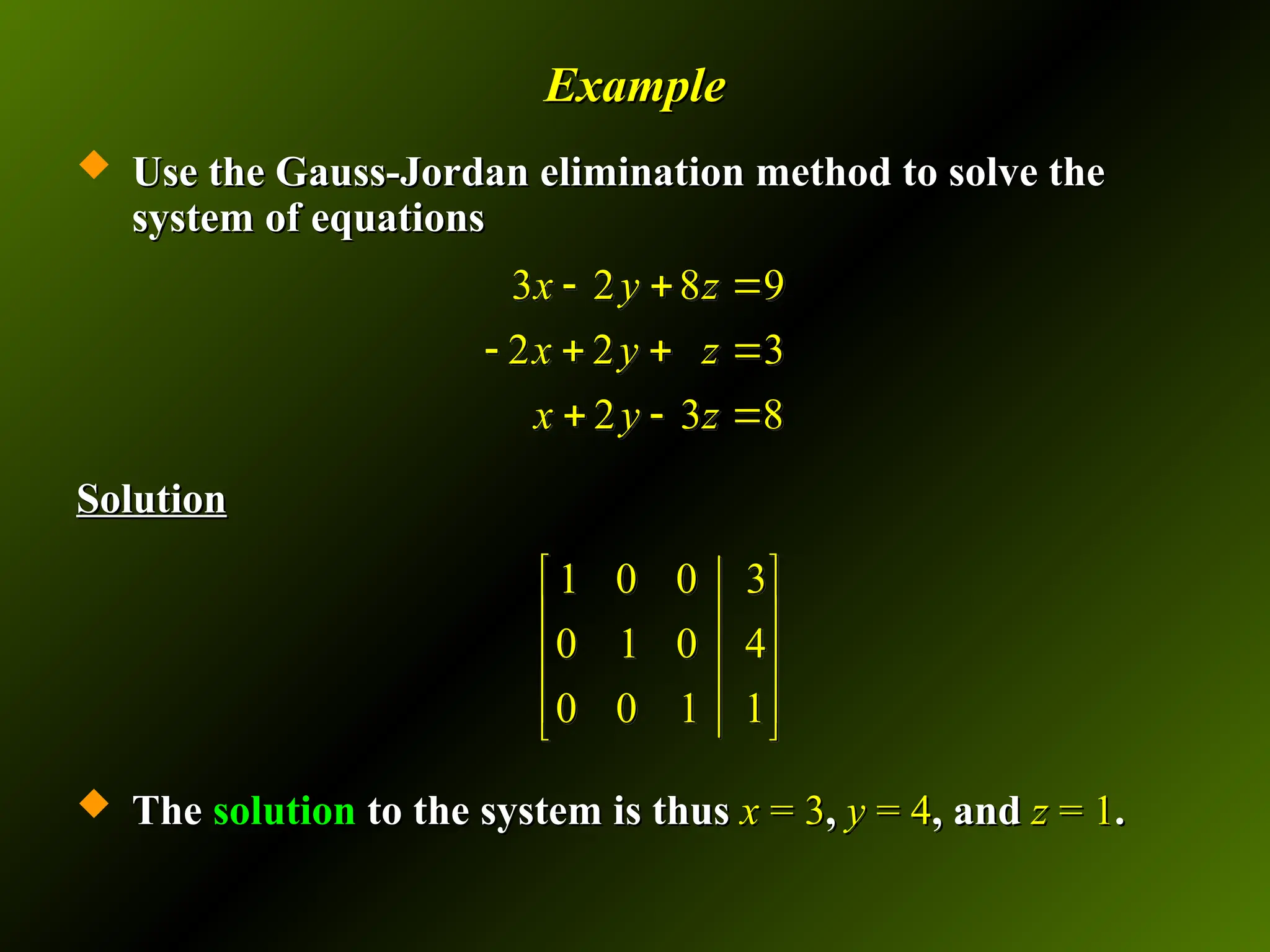
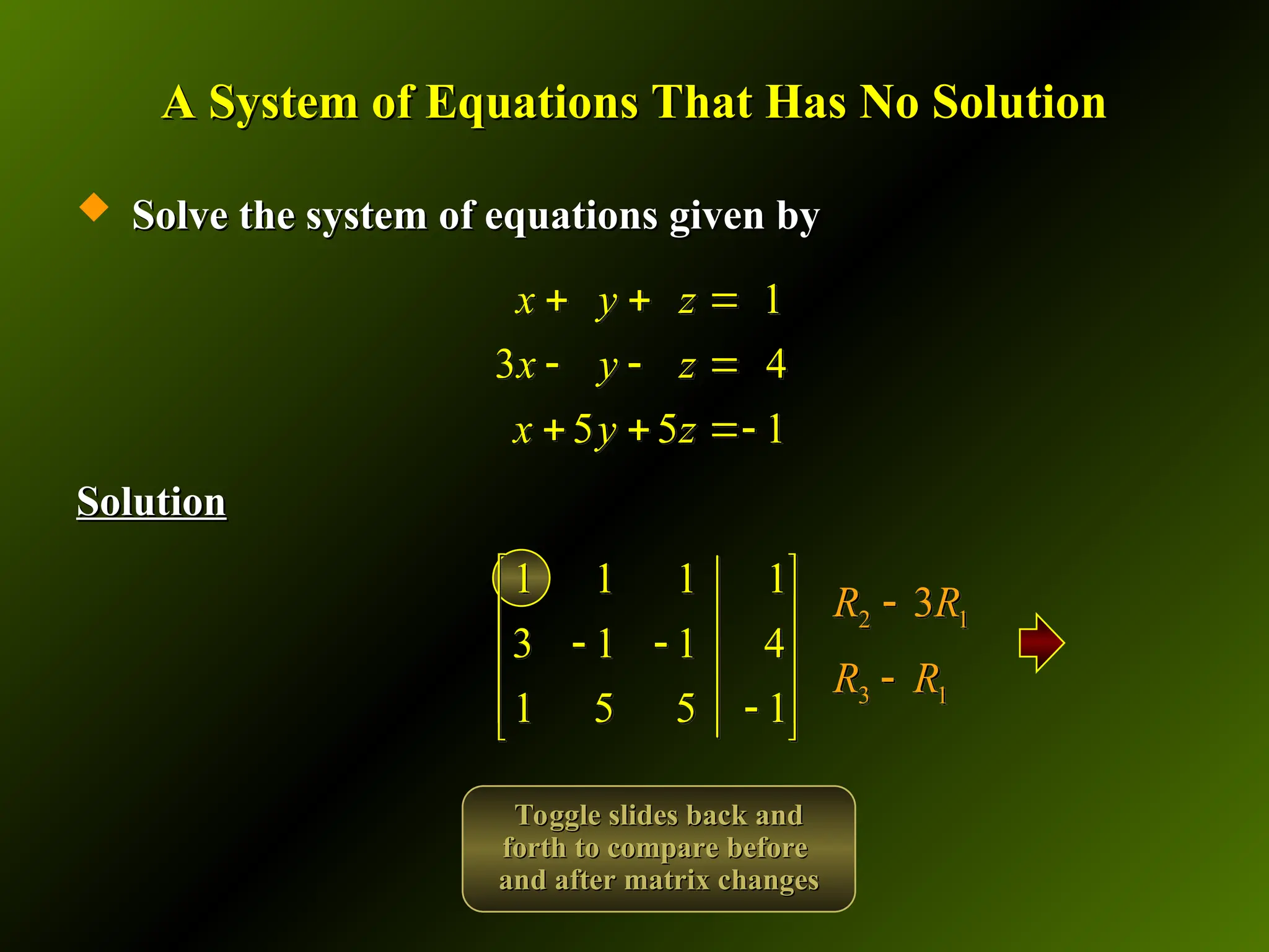
The Gauss-Jordan elimination method is a technique for solving systems of linear equations of any size.
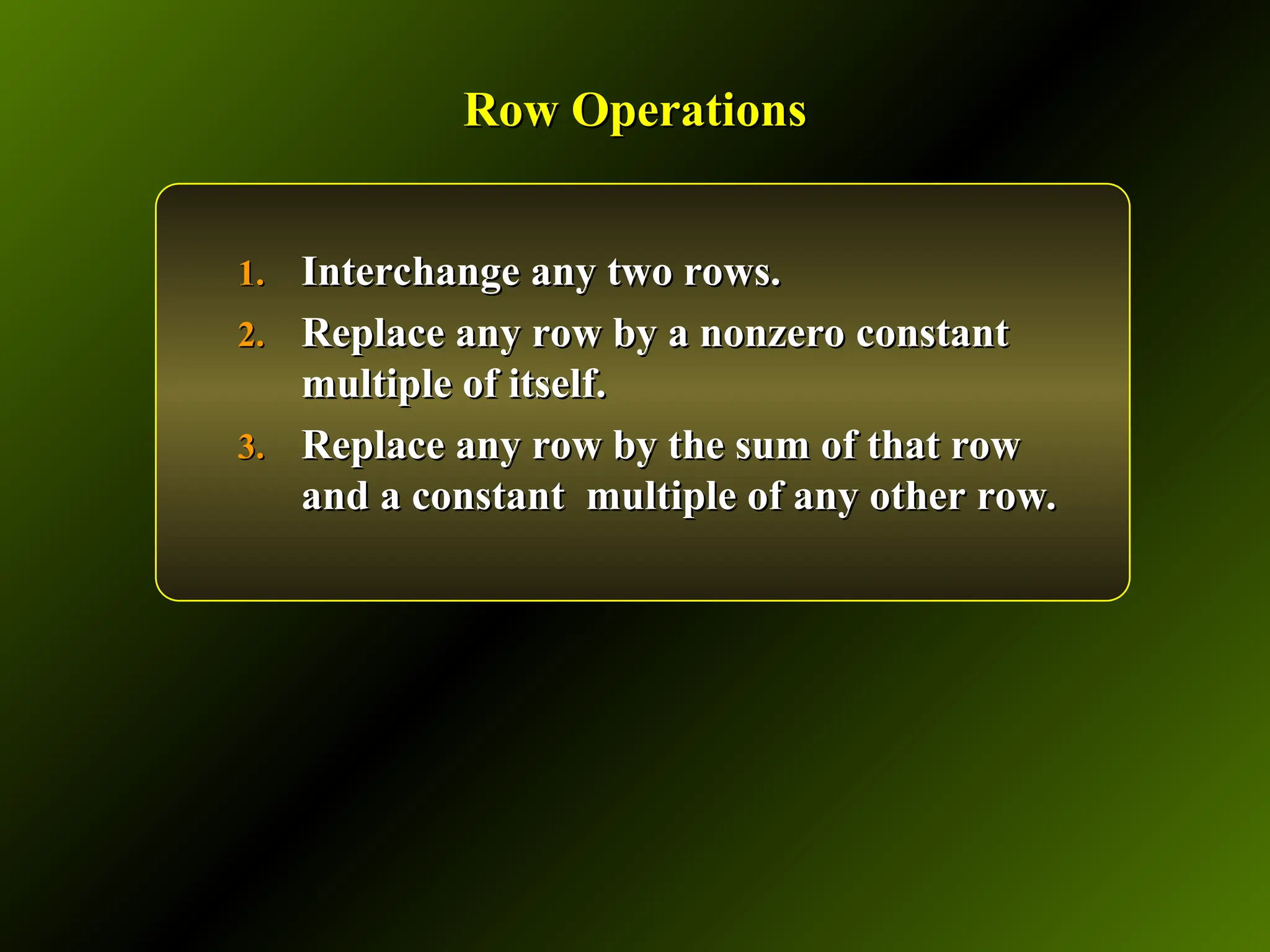
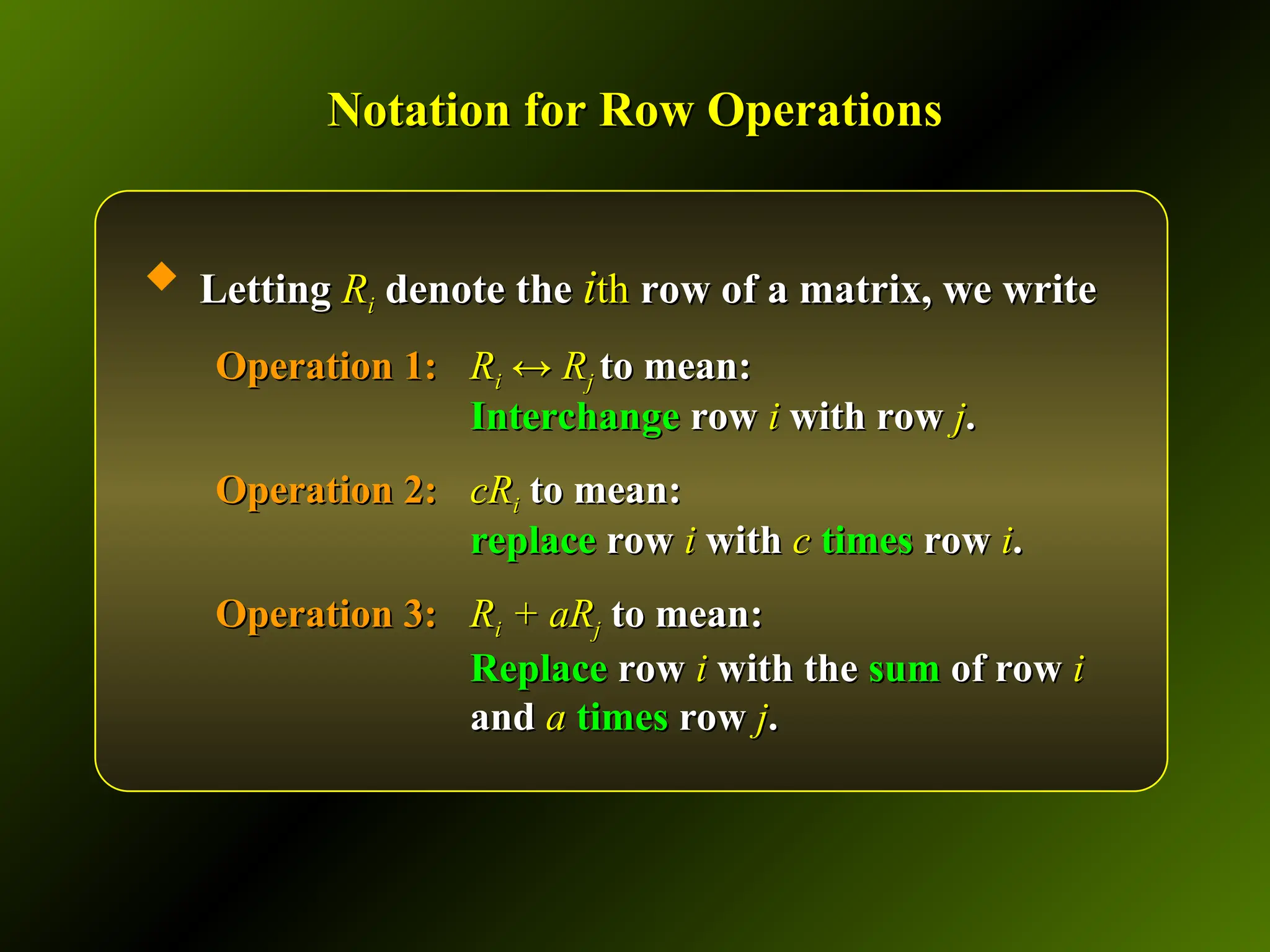
The operations of the Gauss-Jordan method are
Interchange any two equations.
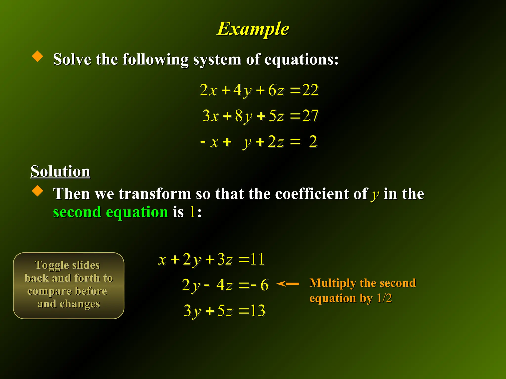
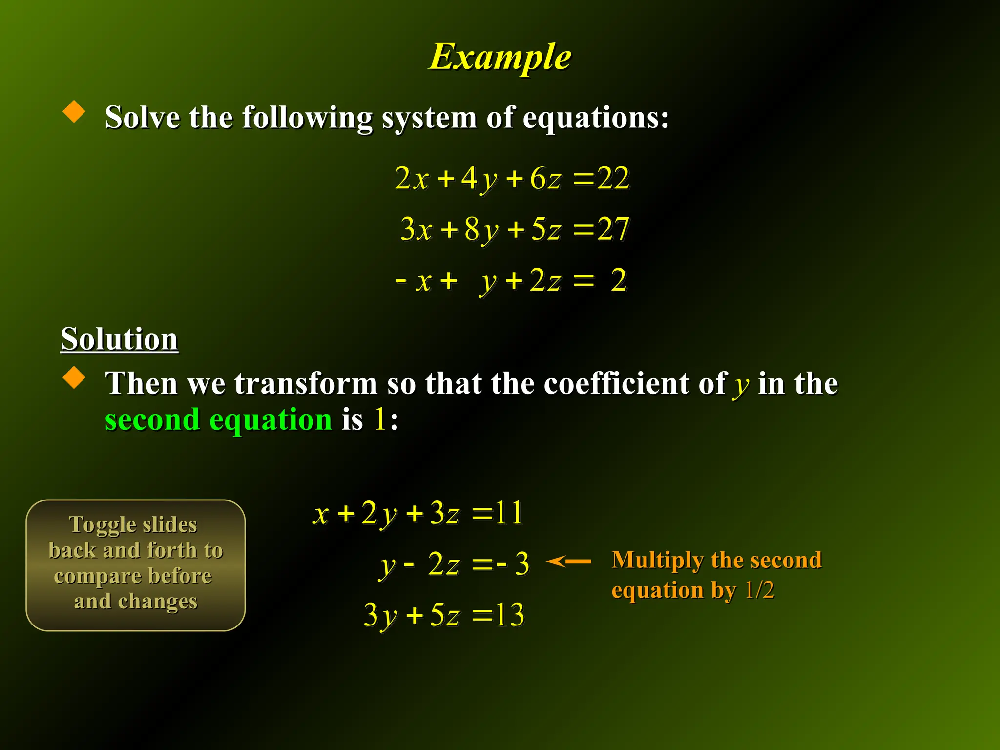
Replace an equation by a nonzero constant multiple of itself.
Replace an equation by the sum of that equation and a constant multiple of any other equation.
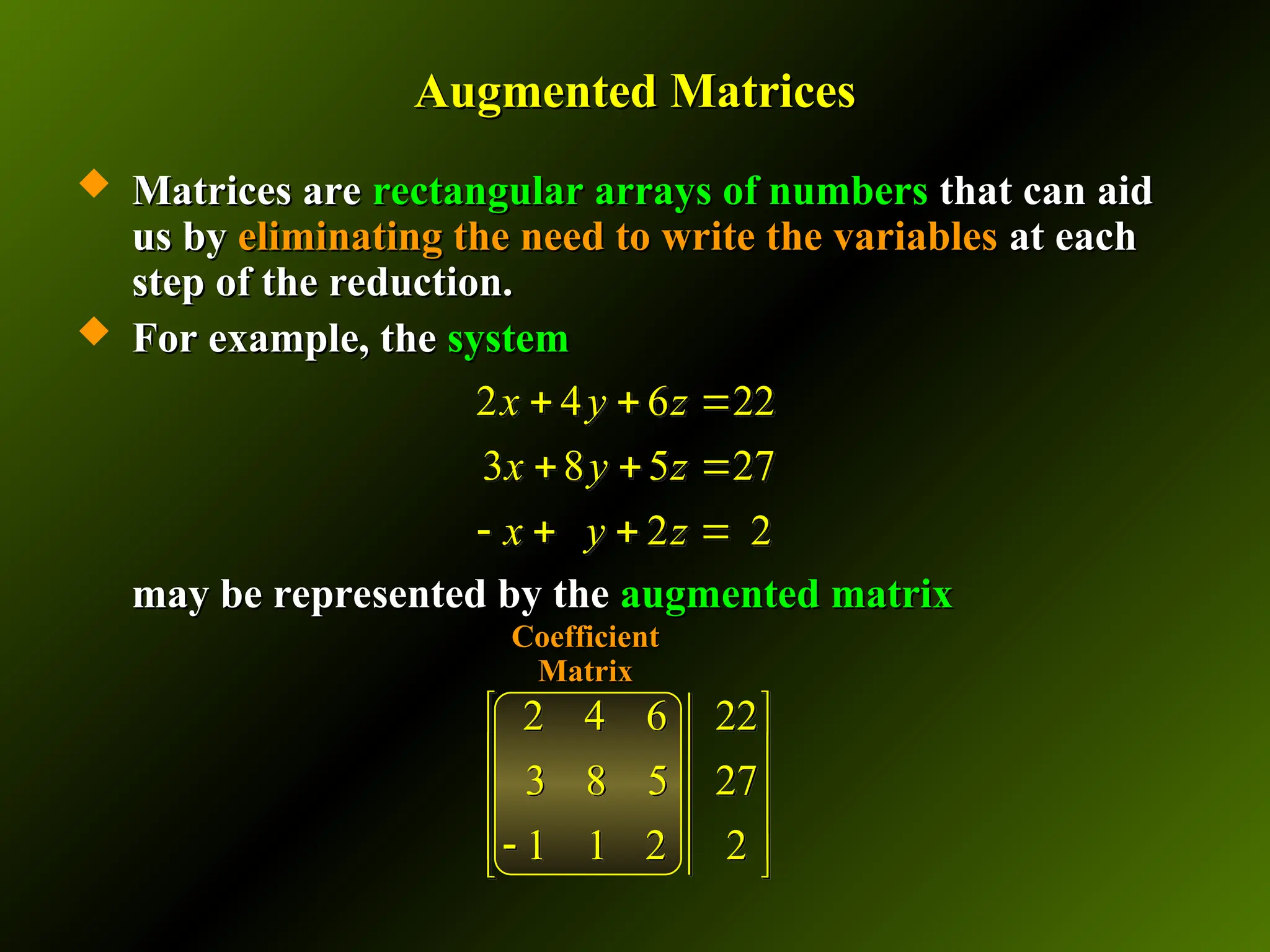
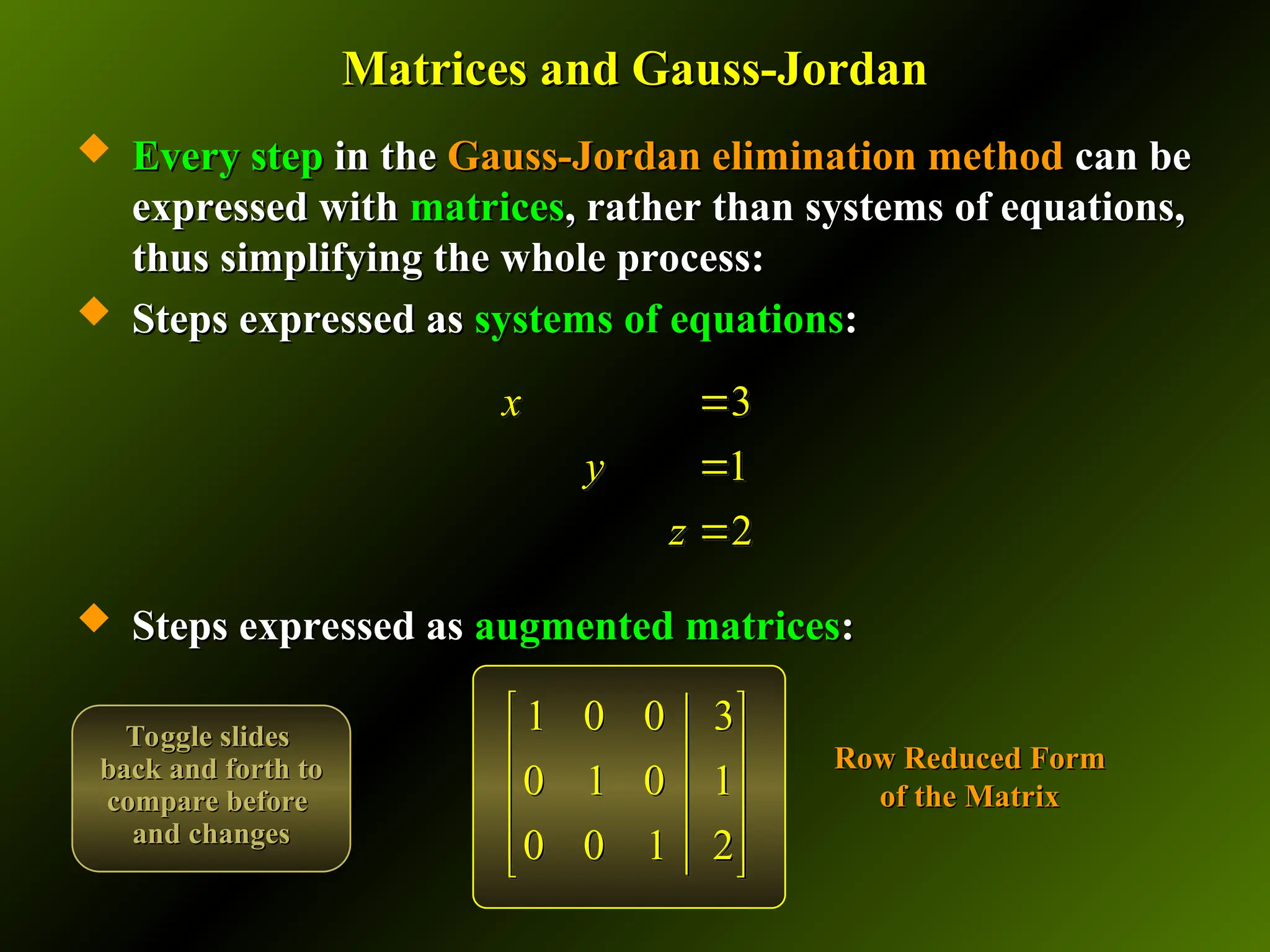
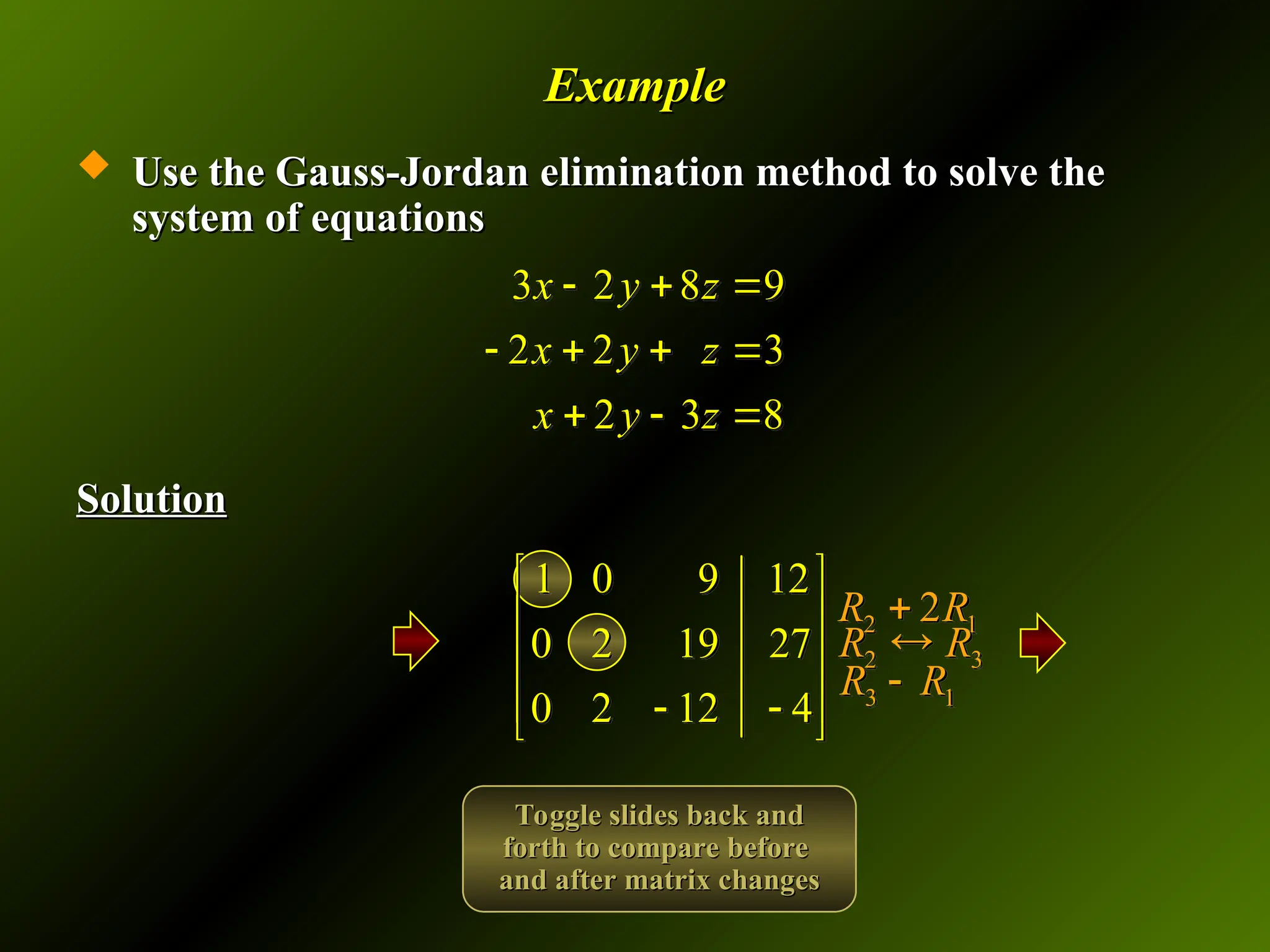
Every step in the Gauss-Jordan elimination method can be expressed with matrices, rather than systems of equations, thus simplifying the whole process:
Steps expressed as systems of equations:
Steps expressed as augmented matrices:
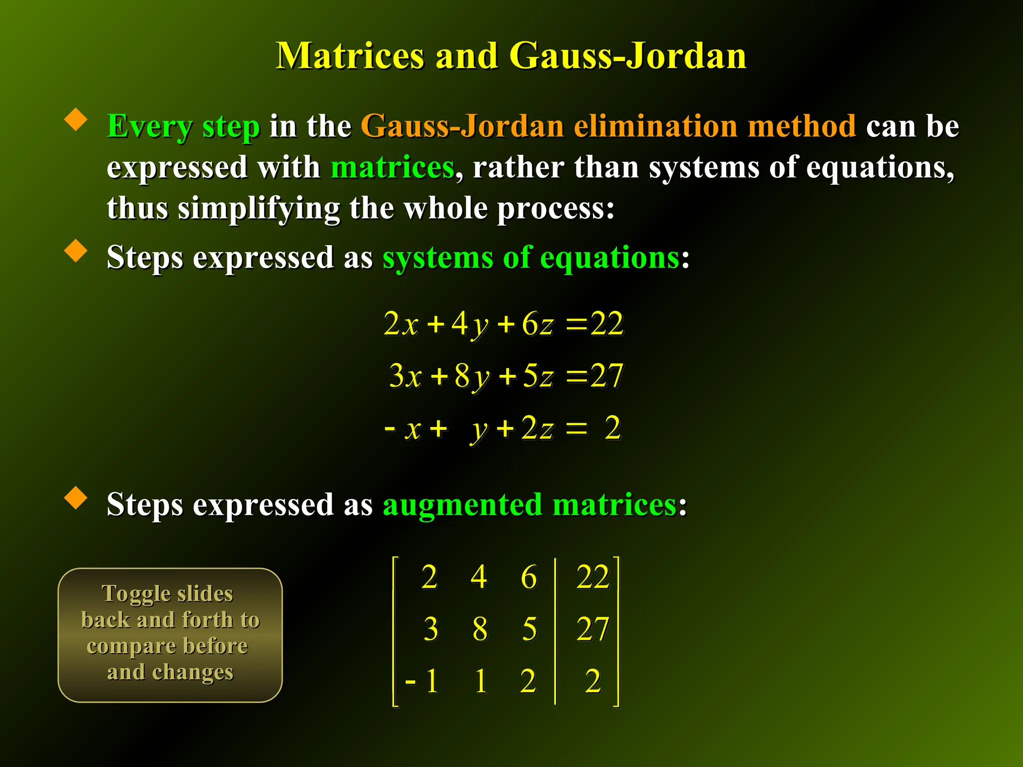
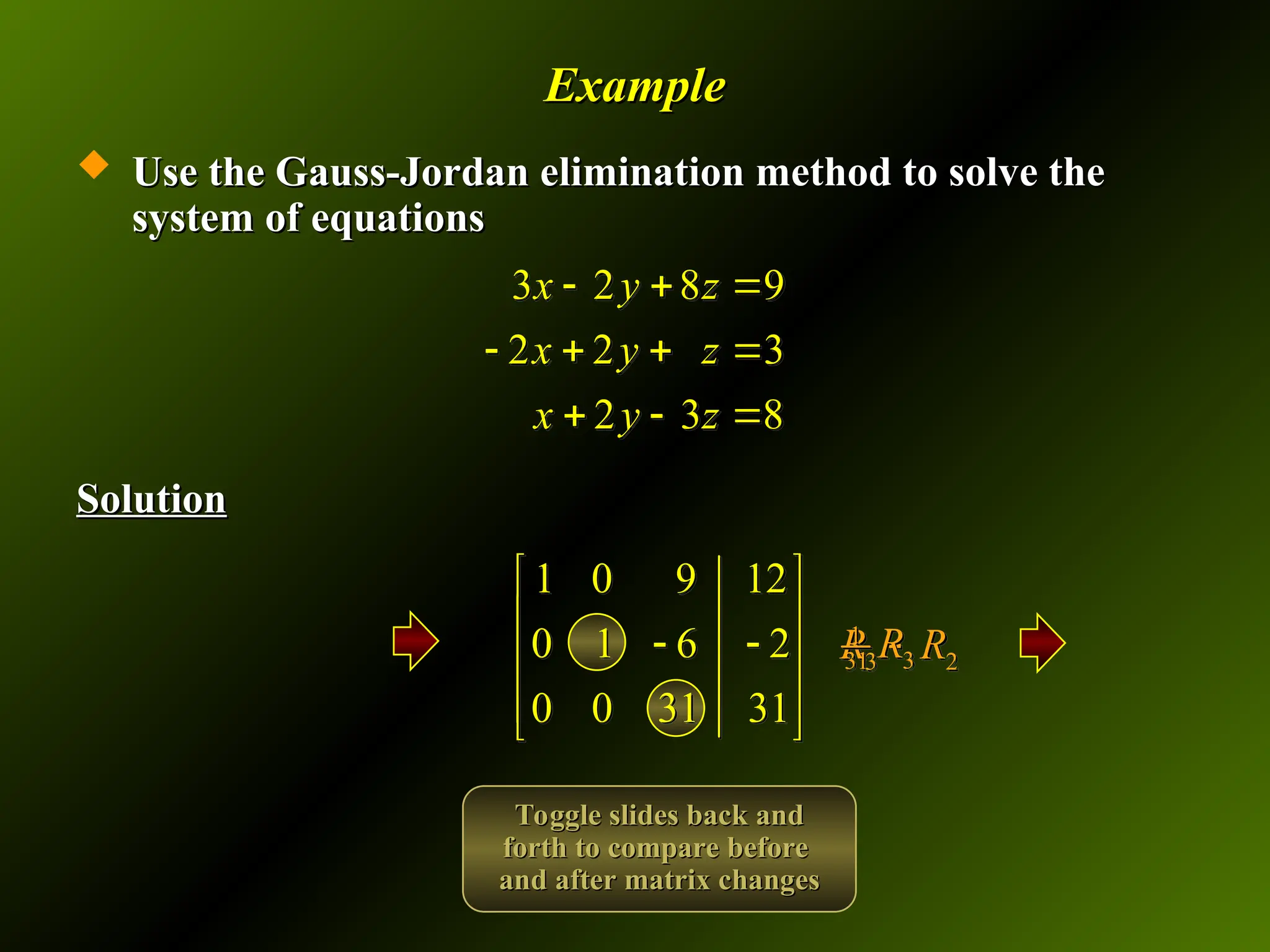
Every step in the Gauss-Jordan elimination method can be expressed with matrices, rather than systems of equations, thus simplifying the whole process:
Steps expressed as systems of equations:
Steps expressed as augmented matrices:
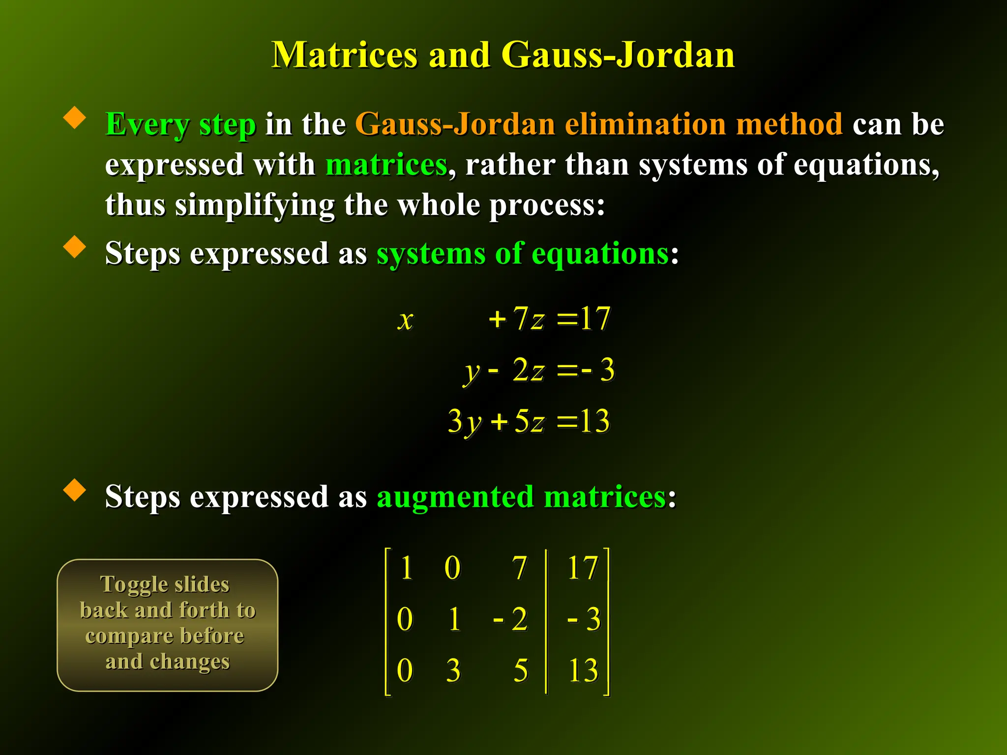
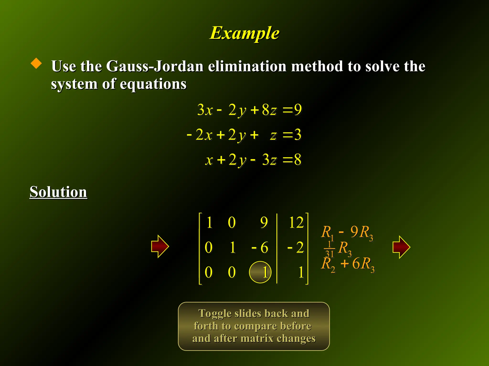
Every step in the Gauss-Jordan elimination method can be expressed with matrices, rather than systems of equations, thus simplifying the whole process:
Steps expressed as systems of equations:
Steps expressed as augmented matrices:
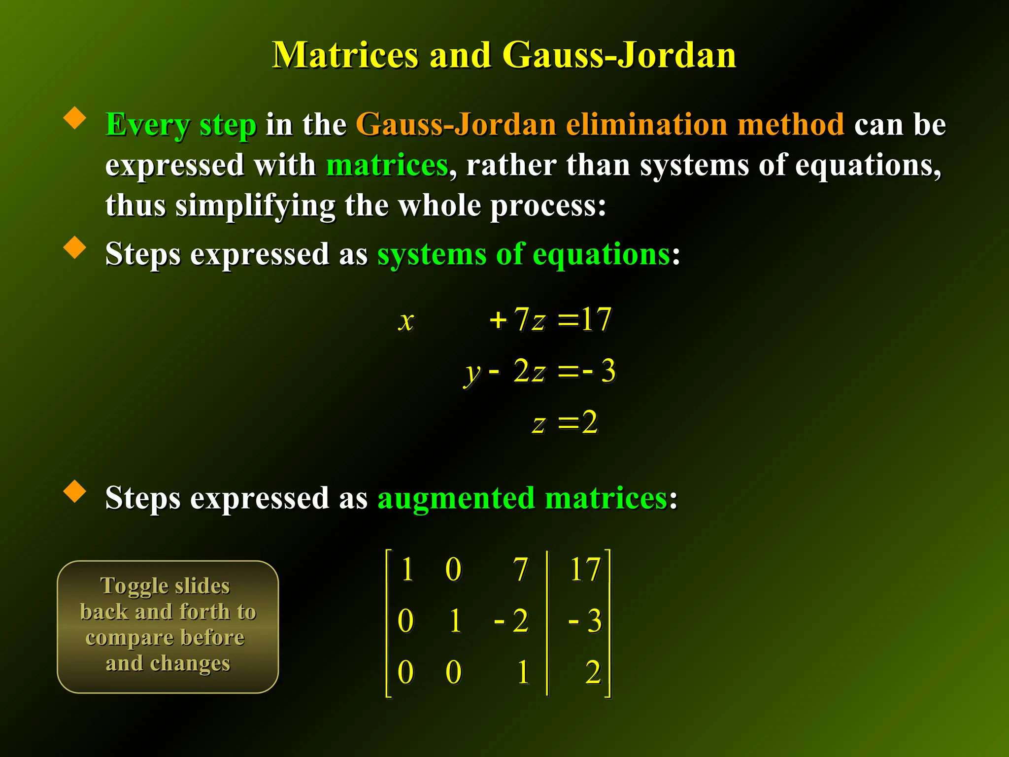
Every step in the Gauss-Jordan elimination method can be expressed with matrices, rather than systems of equations, thus simplifying the whole process:
Steps expressed as systems of equations:
Steps expressed as augmented matrices:
Every step in the Gauss-Jordan elimination method can be expressed with matrices, rather than systems of equations, thus simplifying the whole process:
Steps expressed as systems of equations:
Steps expressed as augmented matrices:
Every step in the Gauss-Jordan elimination method can be expressed with matrices, rather than systems of equations, thus simplifying the whole process:
Steps expressed as systems of equations:
Steps expressed as augmented matrices:
Every step in the Gauss-Jordan elimination method can be expressed with matrices, rather than systems of equations, thus simplifying the whole process:
Steps expressed as systems of equations:


![Multiplying a Row Matrix by a Column Matrix
Multiplying a Row Matrix by a Column Matrix
If we have a
If we have a row matrix
row matrix of size
of size 1
1☓
☓ n
n,
,
And a
And a column matrix
column matrix of size
of size n
n ☓
☓ 1
1,
,
Then we may define the
Then we may define the matrix product
matrix product of
of A
A and
and B
B, written
, written
AB
AB, by
, by
1 2 3
[ ]
n
A a a a a
1
2
3
n
b
b
B b
b
1
2
1 2 3 3 1 1 2 2 3 3
[ ]
n n n
n
b
b
AB a a a a b a b a b a b a b
b
](https://image.slidesharecdn.com/920170928094513pm2-250410093738-7231cbe3/75/Systems-of-Linear-Equations-and-Matrices-ppt-99-2048.jpg)
![Example
Example
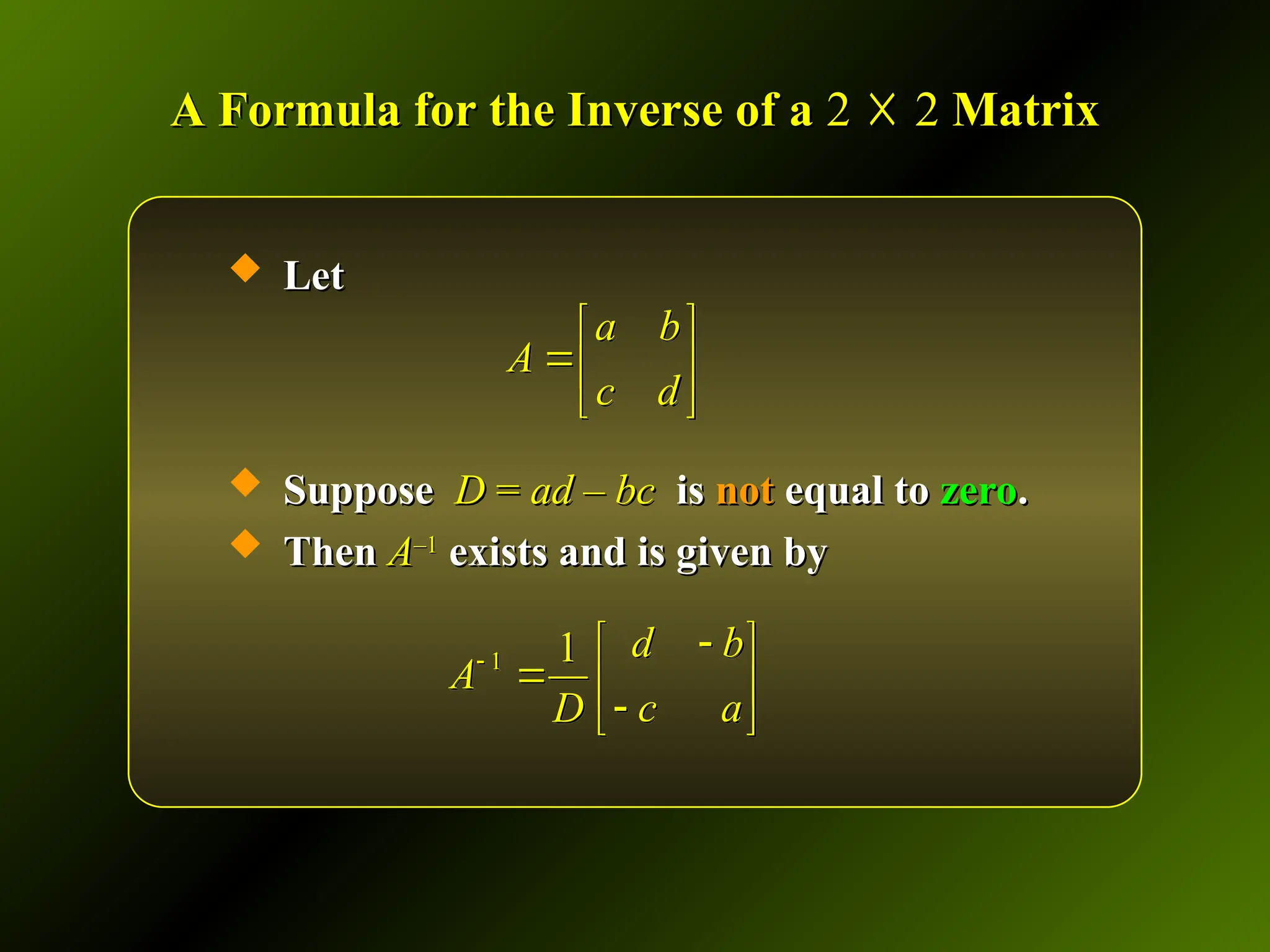
Let
Let
Find the matrix product
Find the matrix product AB
AB.
.
Solution
Solution
2
3
[1 2 3 5]
0
1
a d
n
A B
2
3
[1 2 3 5] (1)(2) ( 2)(3) (3)(0) (5)( 1) 9
0
1
AB
](https://image.slidesharecdn.com/920170928094513pm2-250410093738-7231cbe3/75/Systems-of-Linear-Equations-and-Matrices-ppt-100-2048.jpg)

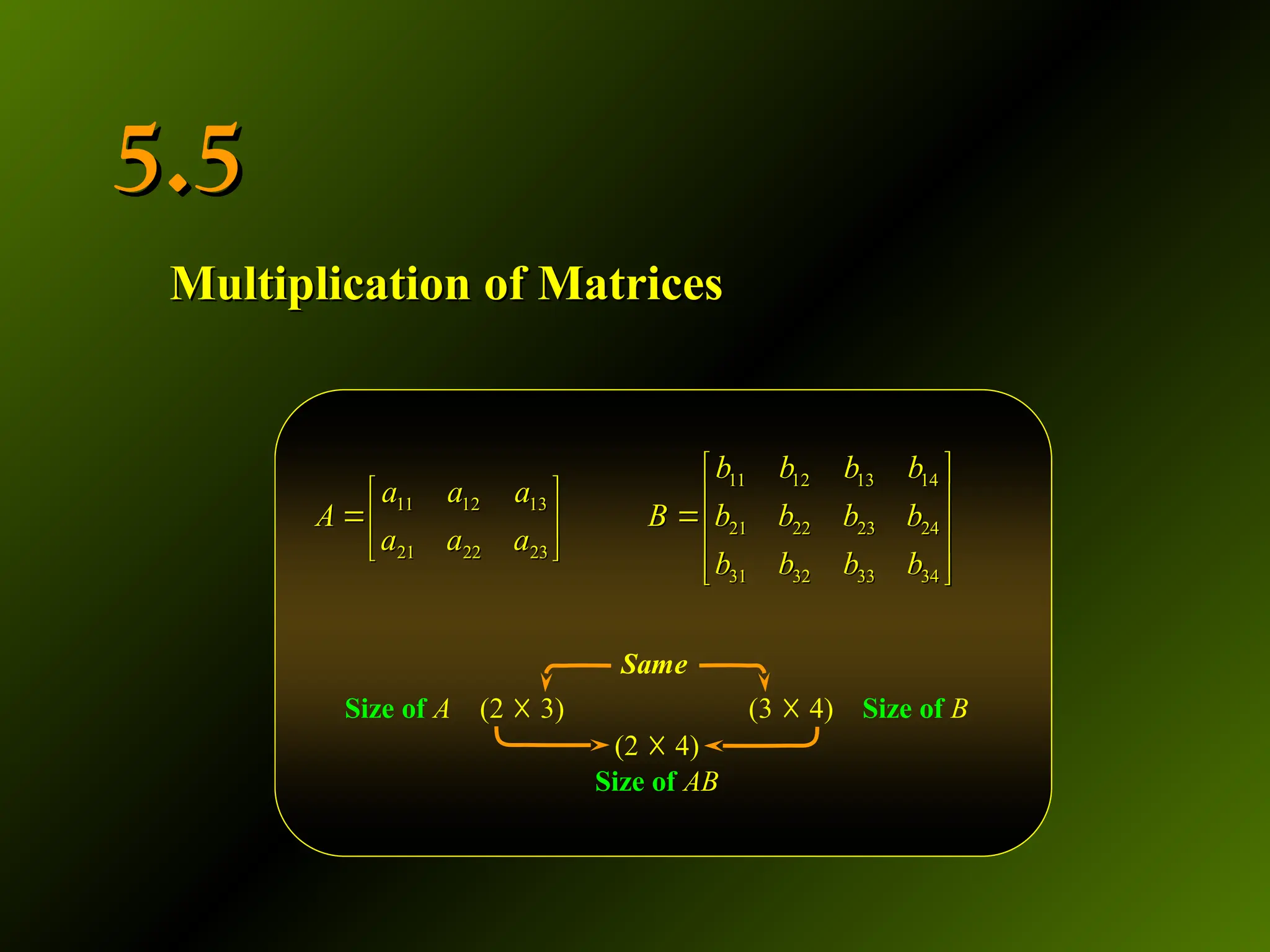
![Mechanics of Matrix Multiplication
Mechanics of Matrix Multiplication
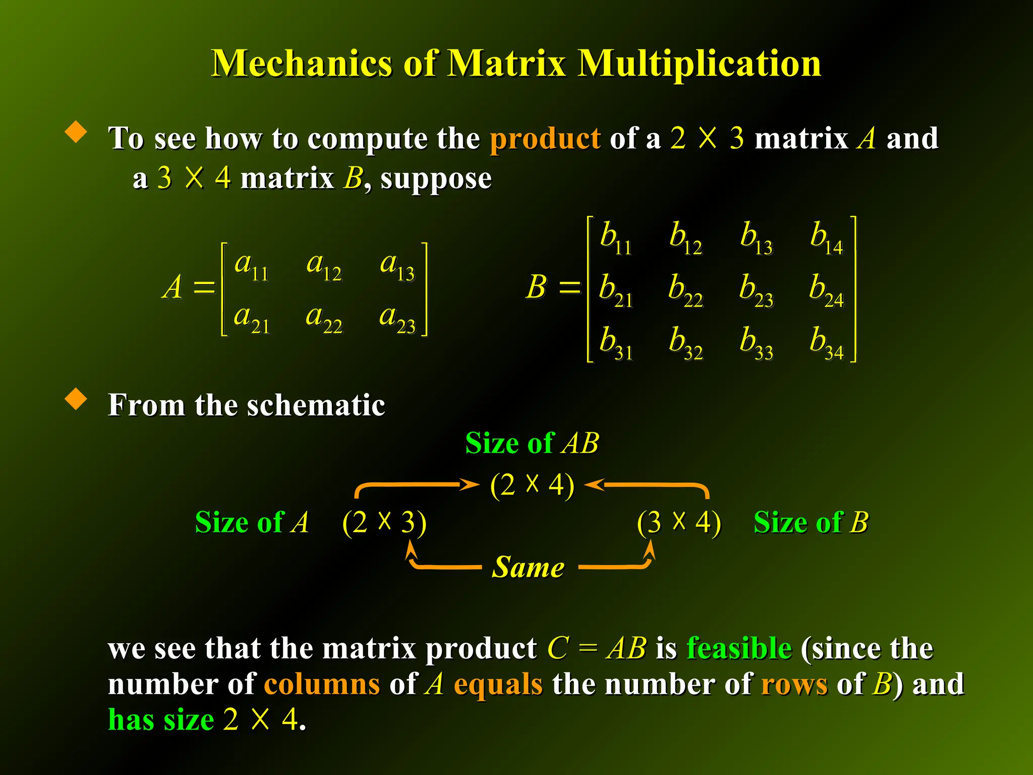
To see how to compute the
To see how to compute the product
product of a
of a 2
2 ☓
☓ 3
3 matrix
matrix A
A and
and
a
a 3
3 ☓
☓ 4
4 matrix
matrix B
B, suppose
, suppose
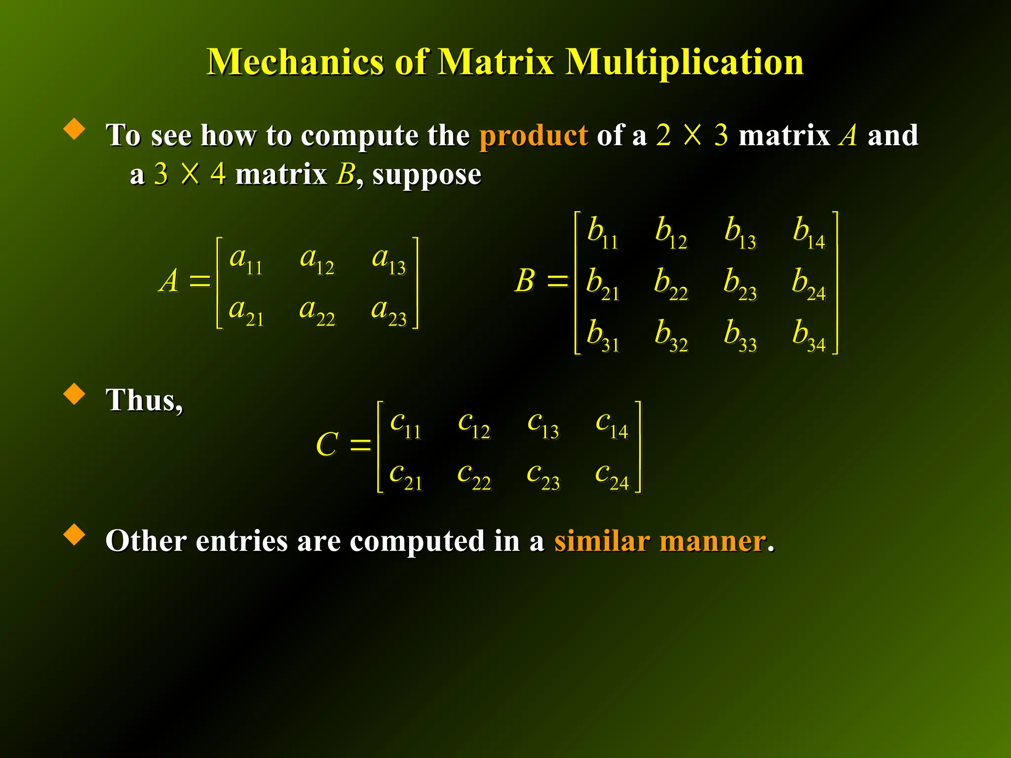
Thus,
Thus,
To see how to
To see how to calculate the entries
calculate the entries of
of C
C consider
consider entry
entry c
c11
11:
:
11 12 13 14
21 22 23 24
c c c c
C
c c c c
11
11 11 12 13 21 11 11 12 21 13 31
31
[ ]
b
c a a a b a b a b a b
b
11 12 13 14
11 12 13
21 22 23 24
21 22 23
31 32 33 34
b b b b
a a a
A B b b b b
a a a
b b b b
](https://image.slidesharecdn.com/920170928094513pm2-250410093738-7231cbe3/75/Systems-of-Linear-Equations-and-Matrices-ppt-105-2048.jpg)
![Mechanics of Matrix Multiplication
Mechanics of Matrix Multiplication
To see how to compute the
To see how to compute the product
product of a
of a 2
2 ☓
☓ 3
3 matrix
matrix A
A and
and
a
a 3
3 ☓
☓ 4
4 matrix
matrix B
B, suppose
, suppose
Thus,
Thus,
Now consider calculating the
Now consider calculating the entry
entry c
c12
12:
:
11 12 13 14
21 22 23 24
c c c c
C
c c c c
12
12 11 12 13 22 11 12 12 22 13 32
32
[ ]
b
c a a a b a b a b a b
b
11 12 13 14
11 12 13
21 22 23 24
21 22 23
31 32 33 34
b b b b
a a a
A B b b b b
a a a
b b b b
](https://image.slidesharecdn.com/920170928094513pm2-250410093738-7231cbe3/75/Systems-of-Linear-Equations-and-Matrices-ppt-106-2048.jpg)
![Mechanics of Matrix Multiplication
Mechanics of Matrix Multiplication
To see how to compute the
To see how to compute the product
product of a
of a 2
2 ☓
☓ 3
3 matrix
matrix A
A and
and
a
a 3
3 ☓
☓ 4
4 matrix
matrix B
B, suppose
, suppose
Thus,
Thus,
Now consider calculating the
Now consider calculating the entry
entry c
c21
21:
:
11 12 13 14
21 22 23 24
c c c c
C
c c c c
11
21 21 22 23 21 21 11 22 21 23 31
31
[ ]
b
c a a a b a b a b a b
b
11 12 13 14
11 12 13
21 22 23 24
21 22 23
31 32 33 34
b b b b
a a a
A B b b b b
a a a
b b b b
](https://image.slidesharecdn.com/920170928094513pm2-250410093738-7231cbe3/75/Systems-of-Linear-Equations-and-Matrices-ppt-107-2048.jpg)
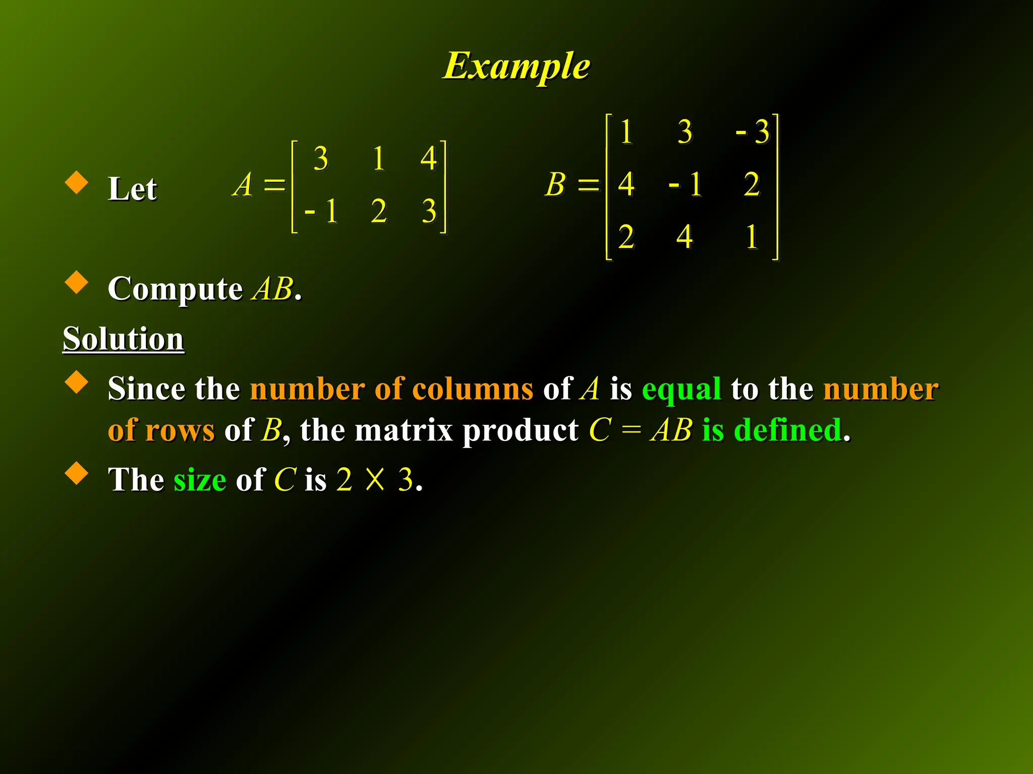
![Example
Example
Let
Let
Compute
Compute AB
AB.
.
Solution
Solution
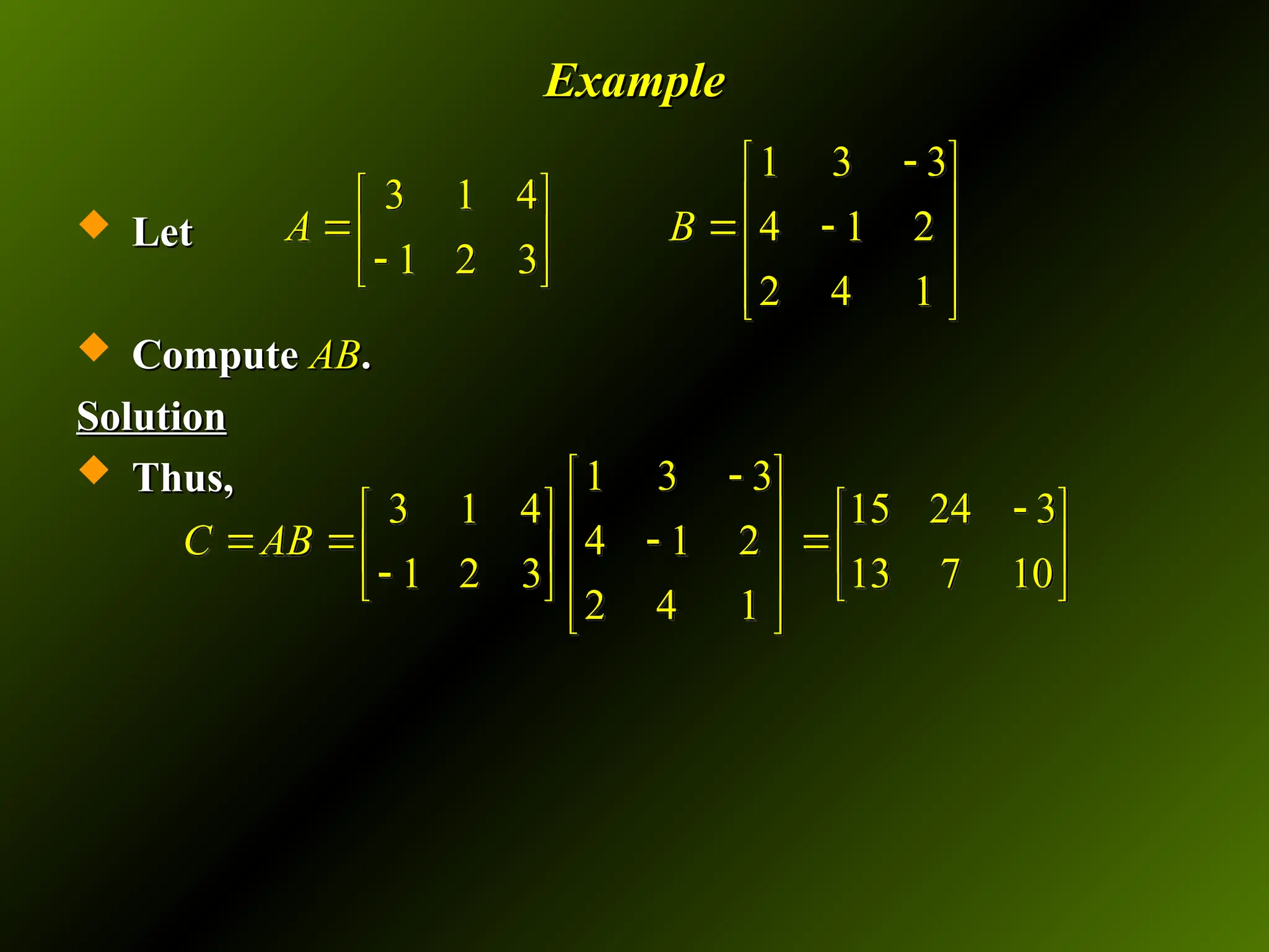
Thus,
Thus,
Calculate all entries for
Calculate all entries for C
C:
:
1 3 3
3 1 4
4 1 2
1 2 3
2 4 1
A B
11 12 13
21 22 23
1 3 3
3 1 4
4 1 2
1 2 3
2 4 1
c c c
C AB
c c c
11
1
[3 1 4] 4 (3)(1) (1)(4) (4)(2) 15
2
c
](https://image.slidesharecdn.com/920170928094513pm2-250410093738-7231cbe3/75/Systems-of-Linear-Equations-and-Matrices-ppt-110-2048.jpg)
![Example
Example
Let
Let
Compute
Compute AB
AB.
.
Solution
Solution
Thus,
Thus,
Calculate all entries for
Calculate all entries for C
C:
:
1 3 3
3 1 4
4 1 2
1 2 3
2 4 1
A B
12 13
21 22 23
1 3 3
15
3 1 4
4 1 2
1 2 3
2 4 1
c c
C AB
c c c
12
3
[3 1 4] 1 (3)(3) (1)( 1) (4)(4) 24
4
c
](https://image.slidesharecdn.com/920170928094513pm2-250410093738-7231cbe3/75/Systems-of-Linear-Equations-and-Matrices-ppt-111-2048.jpg)
![Example
Example
Let
Let
Compute
Compute AB
AB.
.
Solution
Solution
Thus,
Thus,
Calculate all entries for
Calculate all entries for C
C:
:
1 3 3
3 1 4
4 1 2
1 2 3
2 4 1
A B
13
21 22 23
1 3 3
15 24
3 1 4
4 1 2
1 2 3
2 4 1
c
C AB
c c c
13
3
[3 1 4] 2 (3)( 3) (1)(2) (4)(1) 3
1
c
](https://image.slidesharecdn.com/920170928094513pm2-250410093738-7231cbe3/75/Systems-of-Linear-Equations-and-Matrices-ppt-112-2048.jpg)
![Example
Example
Let
Let
Compute
Compute AB
AB.
.
Solution
Solution
Thus,
Thus,
Calculate all entries for
Calculate all entries for C
C:
:
1 3 3
3 1 4
4 1 2
1 2 3
2 4 1
A B
21 22 23
1 3 3
15 24 3
3 1 4
4 1 2
1 2 3
2 4 1
C AB
c c c
21
1
[ 1 2 3] 4 ( 1)(1) (2)(4) (3)(2) 13
2
c
](https://image.slidesharecdn.com/920170928094513pm2-250410093738-7231cbe3/75/Systems-of-Linear-Equations-and-Matrices-ppt-113-2048.jpg)
![Example
Example
Let
Let
Compute
Compute AB
AB.
.
Solution
Solution
Thus,
Thus,
Calculate all entries for
Calculate all entries for C
C:
:
1 3 3
3 1 4
4 1 2
1 2 3
2 4 1
A B
22 23
1 3 3
15 24 3
3 1 4
4 1 2
13
1 2 3
2 4 1
C AB
c c
22
3
[ 1 2 3] 1 ( 1)(3) (2)( 1) (3)(4) 7
4
c
](https://image.slidesharecdn.com/920170928094513pm2-250410093738-7231cbe3/75/Systems-of-Linear-Equations-and-Matrices-ppt-114-2048.jpg)
![Example
Example
Let
Let
Compute
Compute AB
AB.
.
Solution
Solution
Thus,
Thus,
Calculate all entries for
Calculate all entries for C
C:
:
1 3 3
3 1 4
4 1 2
1 2 3
2 4 1
A B
23
1 3 3
15 24 3
3 1 4
4 1 2
13 7
1 2 3
2 4 1
C AB
c
23
3
[ 1 2 3] 2 ( 1)( 3) (2)(2) (3)(1) 10
1
c
](https://image.slidesharecdn.com/920170928094513pm2-250410093738-7231cbe3/75/Systems-of-Linear-Equations-and-Matrices-ppt-115-2048.jpg)
![Finding the Inverse of a Square Matrix
Finding the Inverse of a Square Matrix
Given the
Given the n
n ☓
☓ n
n matrix
matrix A
A:
:
1.
1. Adjoin the
Adjoin the n
n ☓
☓ n
n identity matrix
identity matrix I
I to obtain
to obtain
the
the augmented matrix
augmented matrix [
[A
A |
| I
I ]
].
.
2.
2. Use a sequence of
Use a sequence of row operations
row operations to
to reduce
reduce
[
[A
A |
| I
I ]
] to the form
to the form [
[I
I |
| B
B]
] if possible.
if possible.
Then the matrix
Then the matrix B
B is the
is the inverse
inverse of
of A
A.
.](https://image.slidesharecdn.com/920170928094513pm2-250410093738-7231cbe3/75/Systems-of-Linear-Equations-and-Matrices-ppt-128-2048.jpg)
![Example
Example
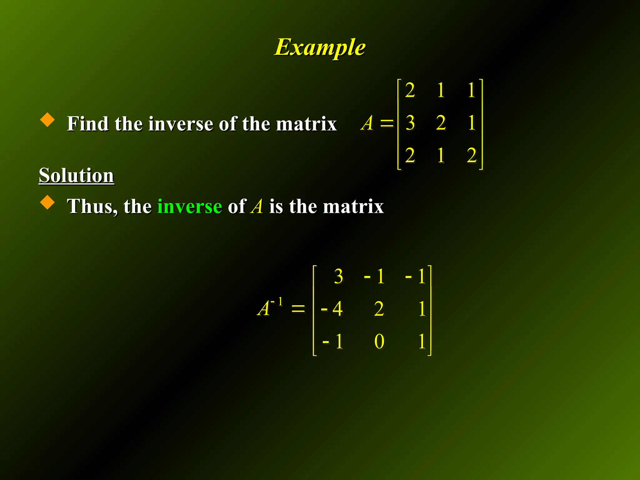
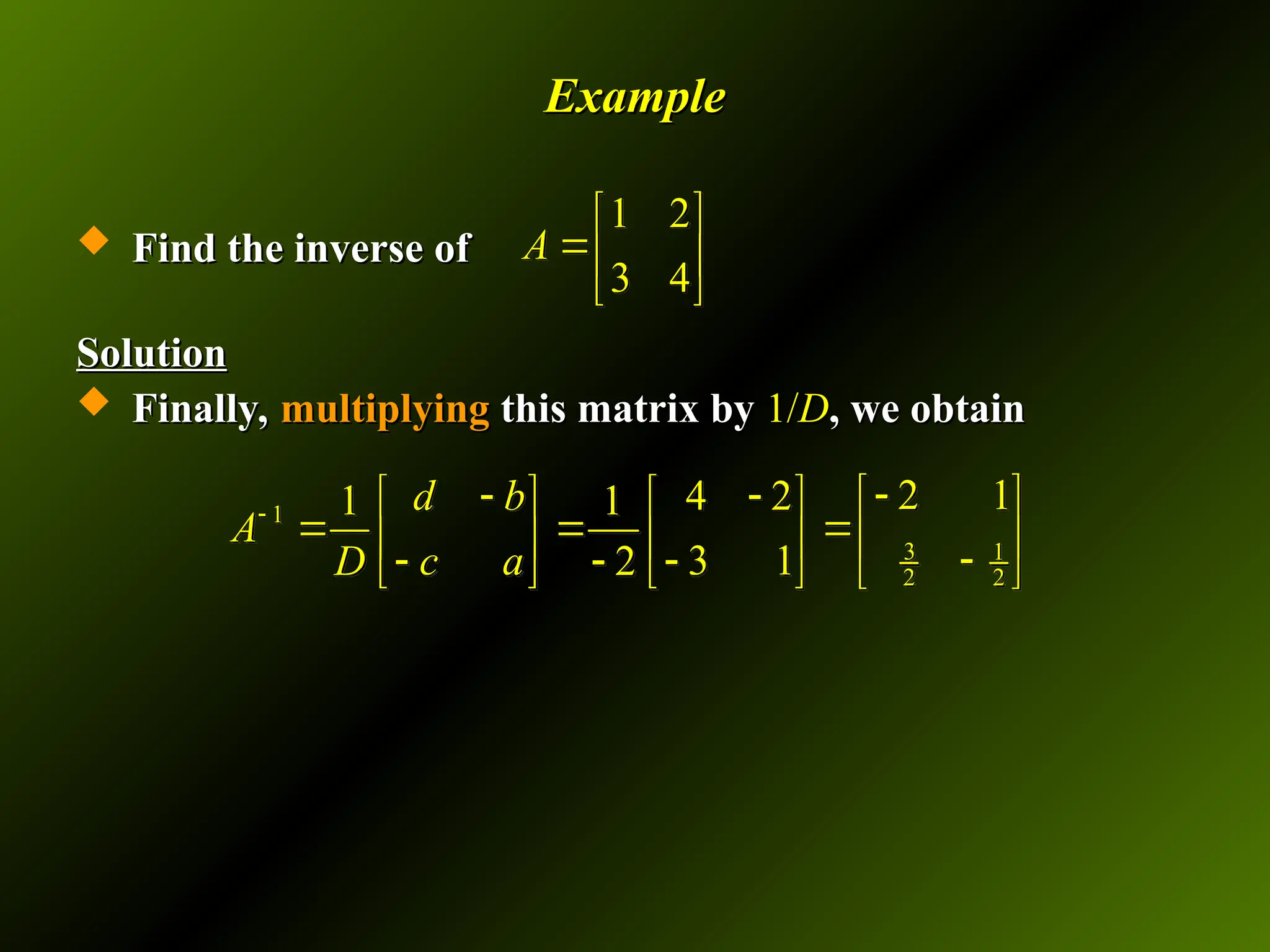
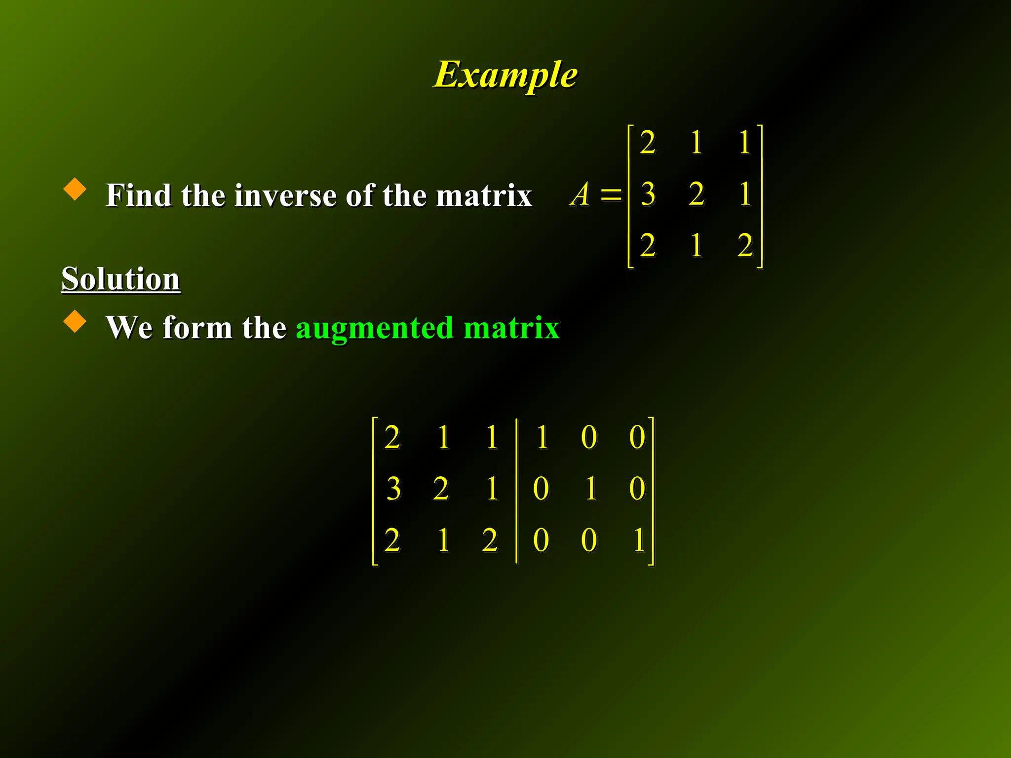
Find the inverse of the matrix
Find the inverse of the matrix
Solution
Solution
And use the
And use the Gauss-Jordan elimination method
Gauss-Jordan elimination method to
to reduce it
reduce it
to the form
to the form [
[I
I |
| B
B]
]:
:
2 1 1
3 2 1
2 1 2
A
2 1 1 1 0 0
3 2 1 0 1 0
2 1 2 0 0 1
1 2
R R
Toggle slides
Toggle slides
back and forth to
back and forth to
compare before
compare before
and changes
and changes](https://image.slidesharecdn.com/920170928094513pm2-250410093738-7231cbe3/75/Systems-of-Linear-Equations-and-Matrices-ppt-130-2048.jpg)
![Example
Example
Find the inverse of the matrix
Find the inverse of the matrix
Solution
Solution
And use the
And use the Gauss-Jordan elimination method
Gauss-Jordan elimination method to
to reduce it
reduce it
to the form
to the form [
[I
I |
| B
B]
]:
:
2 1 1
3 2 1
2 1 2
A
1 1 0 1 1 0
3 2 1 0 1 0
2 1 2 0 0 1
1 2
R R
1
2 3
3 1
3
2
R
R R
R R
Toggle slides
Toggle slides
back and forth to
back and forth to
compare before
compare before
and changes
and changes](https://image.slidesharecdn.com/920170928094513pm2-250410093738-7231cbe3/75/Systems-of-Linear-Equations-and-Matrices-ppt-131-2048.jpg)
![Example
Example
Find the inverse of the matrix
Find the inverse of the matrix
Solution
Solution
And use the
And use the Gauss-Jordan elimination method
Gauss-Jordan elimination method to
to reduce it
reduce it
to the form
to the form [
[I
I |
| B
B]
]:
:
2 1 1
3 2 1
2 1 2
A
1 1 0 1 1 0
0 1 1 3 2 0
0 1 2 2 2 1
1
2 3
3 1
3
2
R
R R
R R
1 2
2
3 2
R R
R
R R
Toggle slides
Toggle slides
back and forth to
back and forth to
compare before
compare before
and changes
and changes](https://image.slidesharecdn.com/920170928094513pm2-250410093738-7231cbe3/75/Systems-of-Linear-Equations-and-Matrices-ppt-132-2048.jpg)
![1 2
2
3 2
R R
R
R R
Example
Example
Find the inverse of the matrix
Find the inverse of the matrix
Solution
Solution
And use the
And use the Gauss-Jordan elimination method
Gauss-Jordan elimination method to
to reduce it
reduce it
to the form
to the form [
[I
I |
| B
B]
]:
:
2 1 1
3 2 1
2 1 2
A
1 0 1 2 1 0
0 1 1 3 2 0
0 0 1 1 0 1
1 3
2 3
R R
R R
Toggle slides
Toggle slides
back and forth to
back and forth to
compare before
compare before
and changes
and changes](https://image.slidesharecdn.com/920170928094513pm2-250410093738-7231cbe3/75/Systems-of-Linear-Equations-and-Matrices-ppt-133-2048.jpg)
![Example
Example
Find the inverse of the matrix
Find the inverse of the matrix
Solution
Solution
And use the
And use the Gauss-Jordan elimination method
Gauss-Jordan elimination method to
to reduce it
reduce it
to the form
to the form [
[I
I |
| B
B]
]:
:
2 1 1
3 2 1
2 1 2
A
1 0 0 3 1 1
0 1 0 4 2 1
0 0 1 1 0 1
1 3
2 3
R R
R R
I
In
n B
B
Toggle slides
Toggle slides
back and forth to
back and forth to
compare before
compare before
and changes
and changes](https://image.slidesharecdn.com/920170928094513pm2-250410093738-7231cbe3/75/Systems-of-Linear-Equations-and-Matrices-ppt-134-2048.jpg)