Math 221 Linear Algebra Le Chen slides summary

1. Math 221: LINEAR ALGEBRA
Chapter 1. Systems of Linear Equations
§1-1. Solutions and Elementary Operations
Le Chen1
Emory University, 2021 Spring
(last updated on 01/25/2021)
Creative Commons License
(CC BY-NC-SA)
1
Slides are adapted from those by Karen Seyffarth from University of Calgary.

2. Solutions of Linear Equations
Elementary Operations
The Augmented Matrix
Solving a System using Back Substitution

3. Solutions of Linear Equations
Elementary Operations
The Augmented Matrix
Solving a System using Back Substitution

4. Solutions of Linear Equations

5. Solutions of Linear Equations
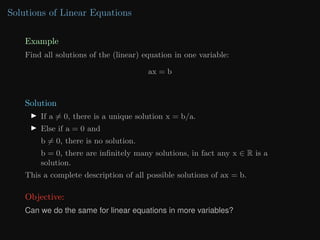
Example
Find all solutions of the (linear) equation in one variable:
ax = b

6. Solutions of Linear Equations
Example
Find all solutions of the (linear) equation in one variable:
ax = b
Solution
I If a 6= 0, there is a unique solution x = b/a.

7. Solutions of Linear Equations
Example
Find all solutions of the (linear) equation in one variable:
ax = b
Solution
I If a 6= 0, there is a unique solution x = b/a.
I Else if a = 0 and
b 6= 0, there is no solution.

8. Solutions of Linear Equations
Example
Find all solutions of the (linear) equation in one variable:
ax = b
Solution
I If a 6= 0, there is a unique solution x = b/a.
I Else if a = 0 and
b 6= 0, there is no solution.
b = 0, there are infinitely many solutions, in fact any x ∈ R is a
solution.
This a complete description of all possible solutions of ax = b.

9. Solutions of Linear Equations
Example
Find all solutions of the (linear) equation in one variable:
ax = b
Solution
I If a 6= 0, there is a unique solution x = b/a.
I Else if a = 0 and
b 6= 0, there is no solution.
b = 0, there are infinitely many solutions, in fact any x ∈ R is a
solution.
This a complete description of all possible solutions of ax = b.
Objective:
Can we do the same for linear equations in more variables?

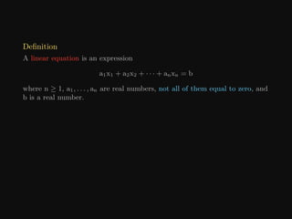
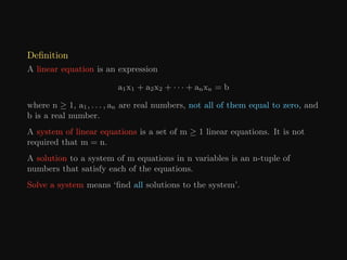
10. Definition
A linear equation is an expression
a1x1 + a2x2 + · · · + anxn = b
where n ≥ 1, a1, . . . , an are real numbers, not all of them equal to zero, and
b is a real number.

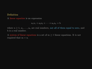
11. Definition
A linear equation is an expression
a1x1 + a2x2 + · · · + anxn = b
where n ≥ 1, a1, . . . , an are real numbers, not all of them equal to zero, and
b is a real number.
A system of linear equations is a set of m ≥ 1 linear equations. It is not
required that m = n.

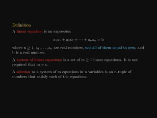
12. Definition
A linear equation is an expression
a1x1 + a2x2 + · · · + anxn = b
where n ≥ 1, a1, . . . , an are real numbers, not all of them equal to zero, and
b is a real number.
A system of linear equations is a set of m ≥ 1 linear equations. It is not
required that m = n.
A solution to a system of m equations in n variables is an n-tuple of
numbers that satisfy each of the equations.

13. Definition
A linear equation is an expression
a1x1 + a2x2 + · · · + anxn = b
where n ≥ 1, a1, . . . , an are real numbers, not all of them equal to zero, and
b is a real number.
A system of linear equations is a set of m ≥ 1 linear equations. It is not
required that m = n.
A solution to a system of m equations in n variables is an n-tuple of
numbers that satisfy each of the equations.
Solve a system means ‘find all solutions to the system’.

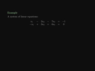
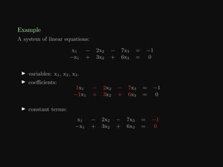
14. Example
A system of linear equations:
x1 − 2x2 − 7x3 = −1
−x1 + 3x2 + 6x3 = 0

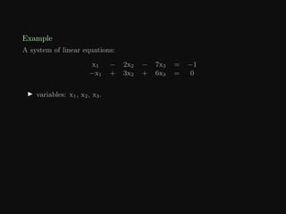
15. Example
A system of linear equations:
x1 − 2x2 − 7x3 = −1
−x1 + 3x2 + 6x3 = 0
I variables: x1, x2, x3.

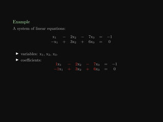
16. Example
A system of linear equations:
x1 − 2x2 − 7x3 = −1
−x1 + 3x2 + 6x3 = 0
I variables: x1, x2, x3.
I coefficients:
1x1 − 2x2 − 7x3 = −1
−1x1 + 3x2 + 6x3 = 0

17. Example
A system of linear equations:
x1 − 2x2 − 7x3 = −1
−x1 + 3x2 + 6x3 = 0
I variables: x1, x2, x3.
I coefficients:
1x1 − 2x2 − 7x3 = −1
−1x1 + 3x2 + 6x3 = 0
I constant terms:
x1 − 2x2 − 7x3 = −1
−x1 + 3x2 + 6x3 = 0

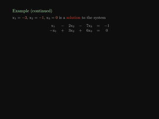
18. Example (continued)
x1 = −3, x2 = −1, x3 = 0 is a solution to the system
x1 − 2x2 − 7x3 = −1
−x1 + 3x2 + 6x3 = 0

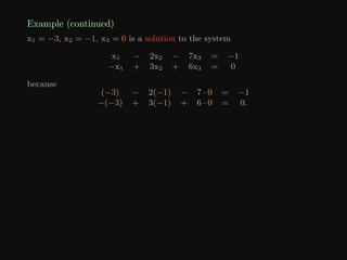
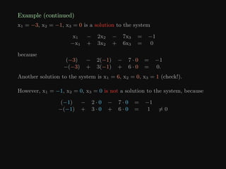
19. Example (continued)
x1 = −3, x2 = −1, x3 = 0 is a solution to the system
x1 − 2x2 − 7x3 = −1
−x1 + 3x2 + 6x3 = 0
because
(−3) − 2(−1) − 7 · 0 = −1
−(−3) + 3(−1) + 6 · 0 = 0.

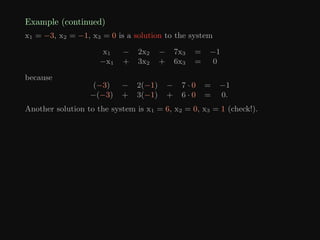
20. Example (continued)
x1 = −3, x2 = −1, x3 = 0 is a solution to the system
x1 − 2x2 − 7x3 = −1
−x1 + 3x2 + 6x3 = 0
because
(−3) − 2(−1) − 7 · 0 = −1
−(−3) + 3(−1) + 6 · 0 = 0.
Another solution to the system is x1 = 6, x2 = 0, x3 = 1 (check!).

21. Example (continued)
x1 = −3, x2 = −1, x3 = 0 is a solution to the system
x1 − 2x2 − 7x3 = −1
−x1 + 3x2 + 6x3 = 0
because
(−3) − 2(−1) − 7 · 0 = −1
−(−3) + 3(−1) + 6 · 0 = 0.
Another solution to the system is x1 = 6, x2 = 0, x3 = 1 (check!).
However, x1 = −1, x2 = 0, x3 = 0 is not a solution to the system, because
(−1) − 2 · 0 − 7 · 0 = −1
−(−1) + 3 · 0 + 6 · 0 = 1 6= 0

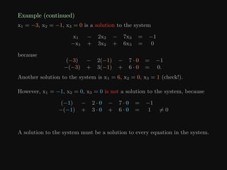
22. Example (continued)
x1 = −3, x2 = −1, x3 = 0 is a solution to the system
x1 − 2x2 − 7x3 = −1
−x1 + 3x2 + 6x3 = 0
because
(−3) − 2(−1) − 7 · 0 = −1
−(−3) + 3(−1) + 6 · 0 = 0.
Another solution to the system is x1 = 6, x2 = 0, x3 = 1 (check!).
However, x1 = −1, x2 = 0, x3 = 0 is not a solution to the system, because
(−1) − 2 · 0 − 7 · 0 = −1
−(−1) + 3 · 0 + 6 · 0 = 1 6= 0
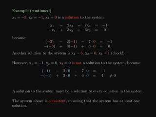
A solution to the system must be a solution to every equation in the system.

23. Example (continued)
x1 = −3, x2 = −1, x3 = 0 is a solution to the system
x1 − 2x2 − 7x3 = −1
−x1 + 3x2 + 6x3 = 0
because
(−3) − 2(−1) − 7 · 0 = −1
−(−3) + 3(−1) + 6 · 0 = 0.
Another solution to the system is x1 = 6, x2 = 0, x3 = 1 (check!).
However, x1 = −1, x2 = 0, x3 = 0 is not a solution to the system, because
(−1) − 2 · 0 − 7 · 0 = −1
−(−1) + 3 · 0 + 6 · 0 = 1 6= 0
A solution to the system must be a solution to every equation in the system.
The system above is consistent, meaning that the system has at least one
solution.

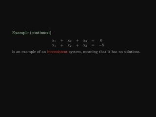
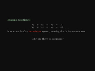
24. Example (continued)
x1 + x2 + x3 = 0
x1 + x2 + x3 = −8
is an example of an inconsistent system, meaning that it has no solutions.

25. Example (continued)
x1 + x2 + x3 = 0
x1 + x2 + x3 = −8
is an example of an inconsistent system, meaning that it has no solutions.
Why are there no solutions?

26. Example
Consider the system of linear equations in two variables
x + y = 3
y − x = 5

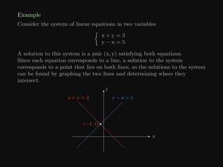
27. Example
Consider the system of linear equations in two variables
x + y = 3
y − x = 5
A solution to this system is a pair (x, y) satisfying both equations.

28. Example
Consider the system of linear equations in two variables
x + y = 3
y − x = 5
A solution to this system is a pair (x, y) satisfying both equations.
Since each equation corresponds to a line, a solution to the system
corresponds to a point that lies on both lines, so the solutions to the system
can be found by graphing the two lines and determining where they
intersect.

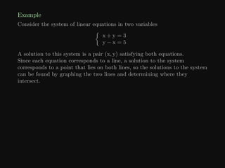
29. Example
Consider the system of linear equations in two variables
x + y = 3
y − x = 5
A solution to this system is a pair (x, y) satisfying both equations.
Since each equation corresponds to a line, a solution to the system
corresponds to a point that lies on both lines, so the solutions to the system
can be found by graphing the two lines and determining where they
intersect.
x
y
y − x = 5
(−1, 4)
x + y = 3

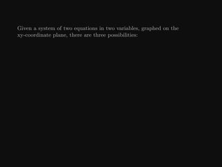
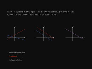
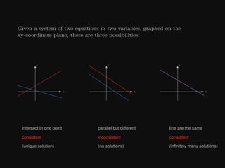
30. Given a system of two equations in two variables, graphed on the
xy-coordinate plane, there are three possibilities:

31. Given a system of two equations in two variables, graphed on the
xy-coordinate plane, there are three possibilities:
x
y
x
y
x
y

32. Given a system of two equations in two variables, graphed on the
xy-coordinate plane, there are three possibilities:
x
y
x
y
x
y
intersect in one point

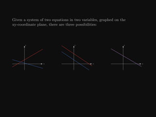
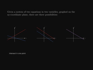
33. Given a system of two equations in two variables, graphed on the
xy-coordinate plane, there are three possibilities:
x
y
x
y
x
y
intersect in one point
consistent
(unique solution)

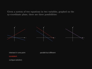
34. Given a system of two equations in two variables, graphed on the
xy-coordinate plane, there are three possibilities:
x
y
x
y
x
y
intersect in one point
consistent
(unique solution)
parallel but different

35. Given a system of two equations in two variables, graphed on the
xy-coordinate plane, there are three possibilities:
x
y
x
y
x
y
intersect in one point
consistent
(unique solution)
parallel but different
inconsistent
(no solutions)

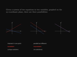
36. Given a system of two equations in two variables, graphed on the
xy-coordinate plane, there are three possibilities:
x
y
x
y
x
y
intersect in one point
consistent
(unique solution)
parallel but different
inconsistent
(no solutions)
line are the same

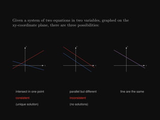
37. Given a system of two equations in two variables, graphed on the
xy-coordinate plane, there are three possibilities:
x
y
x
y
x
y
intersect in one point
consistent
(unique solution)
parallel but different
inconsistent
(no solutions)
line are the same
consistent
(infinitely many solutions)

38. Number of Solutions
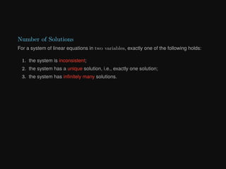
For a system of linear equations in two variables, exactly one of the following holds:

39. Number of Solutions
For a system of linear equations in two variables, exactly one of the following holds:
1. the system is inconsistent;

40. Number of Solutions
For a system of linear equations in two variables, exactly one of the following holds:
1. the system is inconsistent;
2. the system has a unique solution, i.e., exactly one solution;

41. Number of Solutions
For a system of linear equations in two variables, exactly one of the following holds:
1. the system is inconsistent;
2. the system has a unique solution, i.e., exactly one solution;
3. the system has infinitely many solutions.

42. Number of Solutions
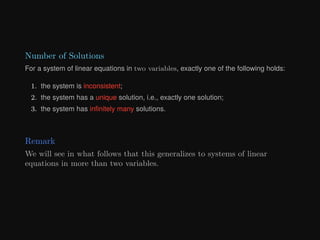
For a system of linear equations in two variables, exactly one of the following holds:
1. the system is inconsistent;
2. the system has a unique solution, i.e., exactly one solution;
3. the system has infinitely many solutions.
Remark
We will see in what follows that this generalizes to systems of linear
equations in more than two variables.

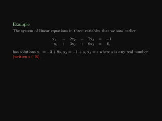
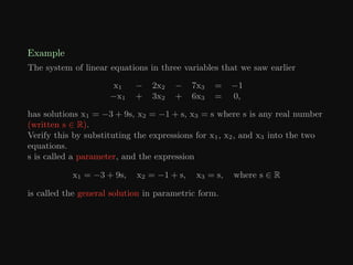
43. Example
The system of linear equations in three variables that we saw earlier
x1 − 2x2 − 7x3 = −1
−x1 + 3x2 + 6x3 = 0,
has solutions x1 = −3 + 9s, x2 = −1 + s, x3 = s where s is any real number
(written s ∈ R).

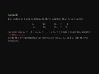
44. Example
The system of linear equations in three variables that we saw earlier
x1 − 2x2 − 7x3 = −1
−x1 + 3x2 + 6x3 = 0,
has solutions x1 = −3 + 9s, x2 = −1 + s, x3 = s where s is any real number
(written s ∈ R).
Verify this by substituting the expressions for x1, x2, and x3 into the two
equations.

45. Example
The system of linear equations in three variables that we saw earlier
x1 − 2x2 − 7x3 = −1
−x1 + 3x2 + 6x3 = 0,
has solutions x1 = −3 + 9s, x2 = −1 + s, x3 = s where s is any real number
(written s ∈ R).
Verify this by substituting the expressions for x1, x2, and x3 into the two
equations.
s is called a parameter, and the expression
x1 = −3 + 9s, x2 = −1 + s, x3 = s, where s ∈ R
is called the general solution in parametric form.

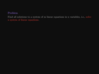
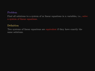
46. Problem
Find all solutions to a system of m linear equations in n variables, i.e., solve
a system of linear equations.

47. Problem
Find all solutions to a system of m linear equations in n variables, i.e., solve
a system of linear equations.
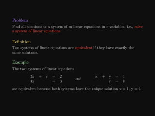
Definition
Two systems of linear equations are equivalent if they have exactly the
same solutions.

48. Problem
Find all solutions to a system of m linear equations in n variables, i.e., solve
a system of linear equations.
Definition
Two systems of linear equations are equivalent if they have exactly the
same solutions.
Example
The two systems of linear equations
2x + y = 2
3x = 3
and
x + y = 1
y = 0
are equivalent because both systems have the unique solution x = 1, y = 0.

49. Solutions of Linear Equations
Elementary Operations
The Augmented Matrix
Solving a System using Back Substitution

50. Elementary Operations

51. Elementary Operations
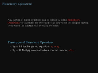
Any system of linear equations can be solved by using Elementary
Operations to transform the system into an equivalent but simpler system
from which the solution can be easily obtained.

52. Elementary Operations
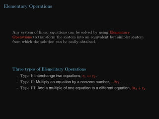
Any system of linear equations can be solved by using Elementary
Operations to transform the system into an equivalent but simpler system
from which the solution can be easily obtained.
Three types of Elementary Operations
– Type I: Interchange two equations, r1 ↔ r2.

53. Elementary Operations
Any system of linear equations can be solved by using Elementary
Operations to transform the system into an equivalent but simpler system
from which the solution can be easily obtained.
Three types of Elementary Operations
– Type I: Interchange two equations, r1 ↔ r2.
– Type II: Multiply an equation by a nonzero number, −2r1.

54. Elementary Operations
Any system of linear equations can be solved by using Elementary
Operations to transform the system into an equivalent but simpler system
from which the solution can be easily obtained.
Three types of Elementary Operations
– Type I: Interchange two equations, r1 ↔ r2.
– Type II: Multiply an equation by a nonzero number, −2r1.
– Type III: Add a multiple of one equation to a different equation, 3r3 + r2.

55. Example
Consider the system of linear eq’s:
3x1 − 2x2 − 7x3 = −1
−x1 + 3x2 + 6x3 = 1
2x1 − x3 = 3

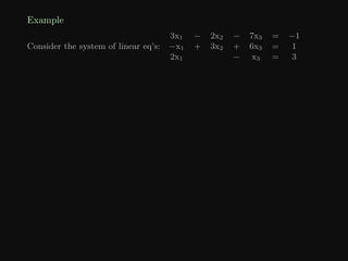
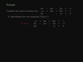
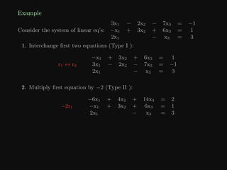
56. Example
Consider the system of linear eq’s:
3x1 − 2x2 − 7x3 = −1
−x1 + 3x2 + 6x3 = 1
2x1 − x3 = 3
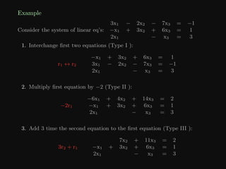
1. Interchange first two equations (Type I ):
r1 ↔ r2
−x1 + 3x2 + 6x3 = 1
3x1 − 2x2 − 7x3 = −1
2x1 − x3 = 3

57. Example
Consider the system of linear eq’s:
3x1 − 2x2 − 7x3 = −1
−x1 + 3x2 + 6x3 = 1
2x1 − x3 = 3
1. Interchange first two equations (Type I ):
r1 ↔ r2
−x1 + 3x2 + 6x3 = 1
3x1 − 2x2 − 7x3 = −1
2x1 − x3 = 3
2. Multiply first equation by −2 (Type II ):
−2r1
−6x1 + 4x2 + 14x3 = 2
−x1 + 3x2 + 6x3 = 1
2x1 − x3 = 3

58. Example
Consider the system of linear eq’s:
3x1 − 2x2 − 7x3 = −1
−x1 + 3x2 + 6x3 = 1
2x1 − x3 = 3
1. Interchange first two equations (Type I ):
r1 ↔ r2
−x1 + 3x2 + 6x3 = 1
3x1 − 2x2 − 7x3 = −1
2x1 − x3 = 3
2. Multiply first equation by −2 (Type II ):
−2r1
−6x1 + 4x2 + 14x3 = 2
−x1 + 3x2 + 6x3 = 1
2x1 − x3 = 3
3. Add 3 time the second equation to the first equation (Type III ):
3r2 + r1
7x2 + 11x3 = 2
−x1 + 3x2 + 6x3 = 1
2x1 − x3 = 3

59. Theorem (Elementary Operations and Solutions)
Suppose that a sequence of elementary operations is performed on a system
of linear equations. Then the resulting system has the same set of solutions
as the original, so the two systems are equivalent.

60. Theorem (Elementary Operations and Solutions)
Suppose that a sequence of elementary operations is performed on a system
of linear equations. Then the resulting system has the same set of solutions
as the original, so the two systems are equivalent.
As a consequence, performing a sequence of elementary operations on a
system of linear equations results in an equivalent system of linear
equations, with the exact same solutions.

61. Solutions of Linear Equations
Elementary Operations
The Augmented Matrix
Solving a System using Back Substitution

62. The Augmented Matrix

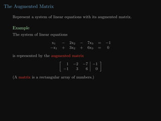
63. The Augmented Matrix
Represent a system of linear equations with its augmented matrix.
Example
The system of linear equations
x1 − 2x2 − 7x3 = −1
−x1 + 3x2 + 6x3 = 0
is represented by the augmented matrix
1 −2 −7 −1
−1 3 6 0
(A matrix is a rectangular array of numbers.)

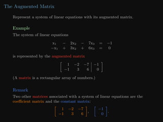
64. The Augmented Matrix
Represent a system of linear equations with its augmented matrix.
Example
The system of linear equations
x1 − 2x2 − 7x3 = −1
−x1 + 3x2 + 6x3 = 0
is represented by the augmented matrix
1 −2 −7 −1
−1 3 6 0
(A matrix is a rectangular array of numbers.)
Remark
Two other matrices associated with a system of linear equations are the
coefficient matrix and the constant matrix:
1 −2 −7
−1 3 6
,
−1
0
.

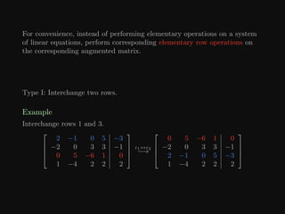
65. For convenience, instead of performing elementary operations on a system
of linear equations, perform corresponding elementary row operations on
the corresponding augmented matrix.

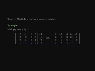
66. For convenience, instead of performing elementary operations on a system
of linear equations, perform corresponding elementary row operations on
the corresponding augmented matrix.
Type I: Interchange two rows.
Example
Interchange rows 1 and 3.




2 −1 0 5 −3
−2 0 3 3 −1
0 5 −6 1 0
1 −4 2 2 2




r1↔r3
−→




0 5 −6 1 0
−2 0 3 3 −1
2 −1 0 5 −3
1 −4 2 2 2





67. Type II: Multiply a row by a nonzero number.
Example
Multiply row 4 by 2.




2 −1 0 5 −3
−2 0 3 3 −1
0 5 −6 1 0
1 −4 2 2 2




2r4
−→




2 −1 0 5 −3
−2 0 3 3 −1
0 5 −6 1 0
2 −8 4 4 4





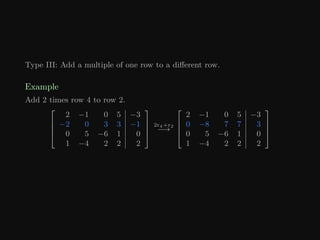
68. Type III: Add a multiple of one row to a different row.
Example
Add 2 times row 4 to row 2.




2 −1 0 5 −3
−2 0 3 3 −1
0 5 −6 1 0
1 −4 2 2 2




2r4+r2
−→




2 −1 0 5 −3
0 −8 7 7 3
0 5 −6 1 0
1 −4 2 2 2





69. Definition
Two matrices A and B are row equivalent (or simply equivalent) if one can
be obtained from the other by a sequence of elementary row operations.

70. Definition
Two matrices A and B are row equivalent (or simply equivalent) if one can
be obtained from the other by a sequence of elementary row operations.
Problem
Prove that A can be obtained from B by a sequence of elementary row
operations if and only if B can be obtained from A by a sequence of
elementary row operations.
Prove that row equivalence is an equivalence relation.

71. Solutions of Linear Equations
Elementary Operations
The Augmented Matrix
Solving a System using Back Substitution

72. Solving a System using Back Substitution

73. Solving a System using Back Substitution
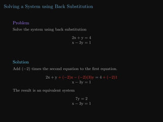
Problem
Solve the system using back substitution
2x + y = 4
x − 3y = 1

74. Solving a System using Back Substitution
Problem
Solve the system using back substitution
2x + y = 4
x − 3y = 1
Solution
Add (−2) times the second equation to the first equation.
2x + y + (−2)x − (−2)(3)y = 4 + (−2)1
x − 3y = 1

75. Solving a System using Back Substitution
Problem
Solve the system using back substitution
2x + y = 4
x − 3y = 1
Solution
Add (−2) times the second equation to the first equation.
2x + y + (−2)x − (−2)(3)y = 4 + (−2)1
x − 3y = 1
The result is an equivalent system
7y = 2
x − 3y = 1

76. Solution (continued)
The first equation of the system,
7y = 2
can be rearranged to give us
y =
2
7
.

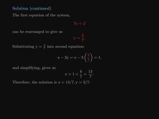
77. Solution (continued)
The first equation of the system,
7y = 2
can be rearranged to give us
y =
2
7
.
Substituting y = 2
7
into second equation:
x − 3y = x − 3
2
7
= 1,

78. Solution (continued)
The first equation of the system,
7y = 2
can be rearranged to give us
y =
2
7
.
Substituting y = 2
7
into second equation:
x − 3y = x − 3
2
7
= 1,
and simplifying, gives us
x = 1 +
6
7
=
13
7
.

79. Solution (continued)
The first equation of the system,
7y = 2
can be rearranged to give us
y =
2
7
.
Substituting y = 2
7
into second equation:
x − 3y = x − 3
2
7
= 1,
and simplifying, gives us
x = 1 +
6
7
=
13
7
.
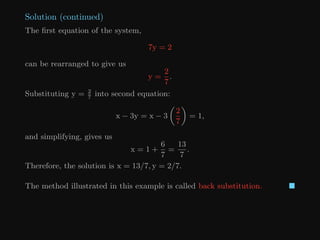
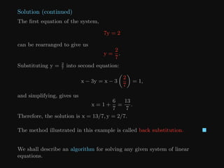
Therefore, the solution is x = 13/7, y = 2/7.

80. Solution (continued)
The first equation of the system,
7y = 2
can be rearranged to give us
y =
2
7
.
Substituting y = 2
7
into second equation:
x − 3y = x − 3
2
7
= 1,
and simplifying, gives us
x = 1 +
6
7
=
13
7
.
Therefore, the solution is x = 13/7, y = 2/7.
The method illustrated in this example is called back substitution.

81. Solution (continued)
The first equation of the system,
7y = 2
can be rearranged to give us
y =
2
7
.
Substituting y = 2
7
into second equation:
x − 3y = x − 3
2
7
= 1,
and simplifying, gives us
x = 1 +
6
7
=
13
7
.
Therefore, the solution is x = 13/7, y = 2/7.
The method illustrated in this example is called back substitution.
We shall describe an algorithm for solving any given system of linear
equations.