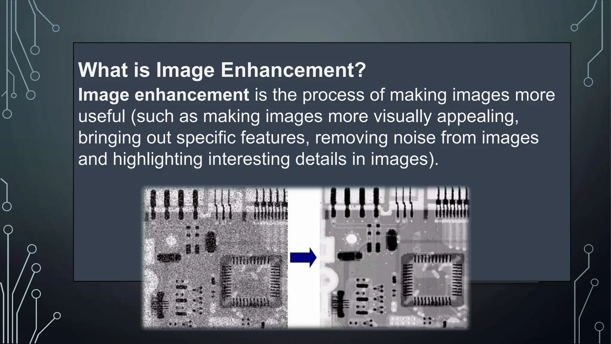
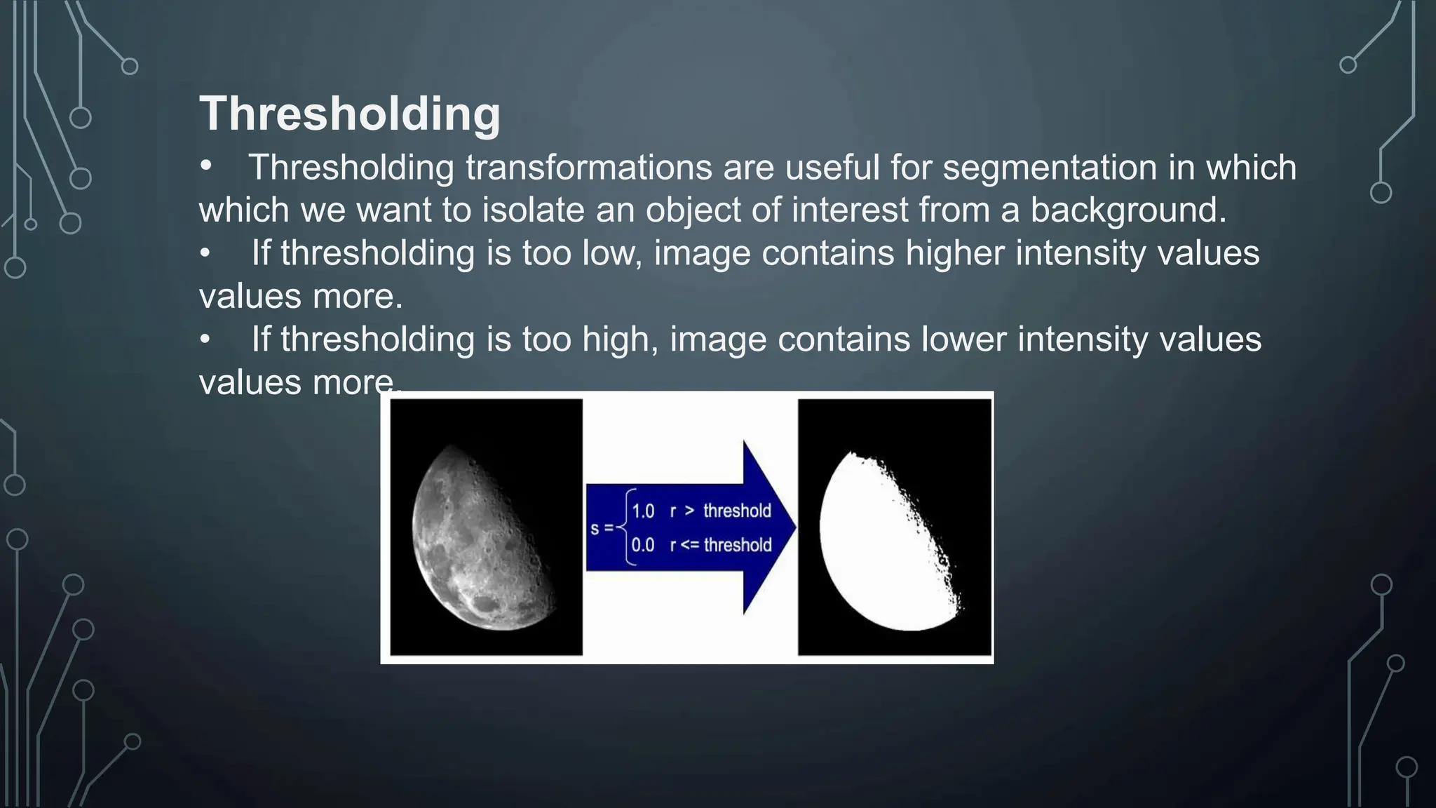
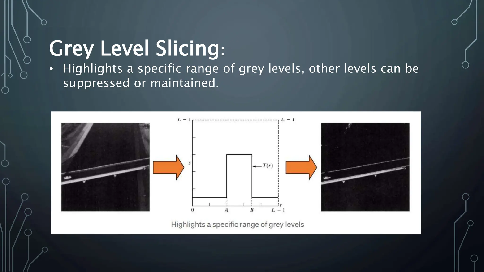
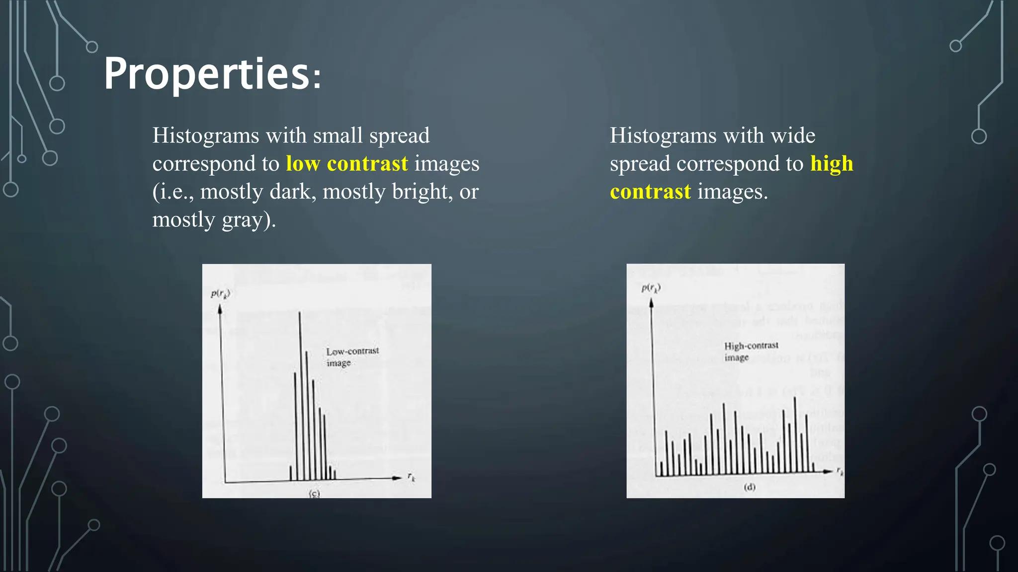
The document discusses image enhancement, defining it as the process of making images more useful and visually appealing. It outlines various techniques such as spatial and frequency domain methods, along with specific operations like histogram equalization and grey level transformations. The future trends in image enhancement include applications of artificial intelligence, real-time processing, and integration with augmented and virtual reality.

1. IMAGE ENHANCEMENT
PRESENTED TO: DR. SAFIULLAH

2. CONTENTS
Introduction
Techniques
Applications
Future Trends

3. SAIRA EJAZ
23015956-017

4. What is Image Enhancement?
Image enhancement is the process of making images more
useful (such as making images more visually appealing,
bringing out specific features, removing noise from images
and highlighting interesting details in images).

5. TECHNIQUES
Spatial
domain
Frequency
domain

6. • Spatial domain techniques: manipulates the pixels of
an image directly. This process happens in the image’s
coordinate system, also known as the spatial domain.
• Frequency domain techniques: transforms an image
from the spatial domain to the frequency domain. In this
process, Mathematical transformations (such as the Fourier
transform) are used. The image can be modified by
manipulating its frequency components.

7. Most spatial domain
enhancement operations can
be reduced to the form g (x, y)
= T[ f (x, y)] where f (x, y) is
the input image, g (x, y) is the
processed image and T is
some operator defined over
some neighbourhood of (x,
y). For example- operation
T(say, addition of 5 to all the
pixel) is carried out in I(x,y)
which means that each pixel
value is increased by 5. where,
I’(x,y) is the new intensity
after adding 5 to I(x,y)

8. Point Processing Techniques
1. Negative Images
2. Thresholding
3. Some of The Grey Level
Transformations

9. Negative Images:
• Negative images are useful for
enhancing details.
• s = intensity_max — r

10. Thresholding
• Thresholding transformations are useful for segmentation in which
which we want to isolate an object of interest from a background.
• If thresholding is too low, image contains higher intensity values
values more.
• If thresholding is too high, image contains lower intensity values
values more.

11. HIJAB ZAINAB
23015956-004

12. Some Of Grey Level Transformations:
• Linear
Negative/Identity
• Logarithmic
Log/Inverse log
• Power law
nth power/ nth root

13. Identity:
Each value of the input image is directly mapped to
the corresponding value of the output image. That
results in the same input image and output image.

14. Logarithmic:
• The general form of the log transformation is
• The log transformation maps a narrow range of low input
grey level values into a wider range of output values.
• The inverse log transformation performs the opposite
transformation.
• Log functions are particularly useful when the input grey
level values may have an extremely large range of values.
( ) ( )
r
c
r
T
s +
=
= 1
log

15. Power Law (Gamma Correction):
• Power law transformations have the following form:
• Map a narrow range of dark input values into a wider range
of output values or vice versa.
• Varying γ gives a whole family of curves.

16. Power Law:

17. Piecewise Linear Transformation
Functions:
Contrast Stretching or Compression
o Stretch gray-level ranges where we desire more information
(slope > 1)
o Compress gray-level ranges that are of little interest
(0 < slope < 1)

18. Grey Level Slicing:
• Highlights a specific range of grey levels, other levels can be
suppressed or maintained.

19. Bit Plane Slicing:
• By isolating particular bits of the pixel values in an image we
can highlight interesting aspects of that image.
• Higher-order bits usually contain most of the significant
visual information.
• Lower-order bits contain subtle details.

20. Bit Plane Slicing:

21. SALVA SADIQ
23015956-014

22. Histogram Equalization:
• Histogram equalization is a technique used to
improve the contrast of an image by redistributing
its pixel intensity values.
Goal:
• To achieve a uniform distribution of intensities,
thereby enhancing the overall contrast of the
image.
• A graphical representation of the distribution of
pixel intensity values in an image.
• X-axis represents the intensity values (from 0 to
255 for an 8-bit image)
• Y-axis represents the number of pixels with each

23. Steps in Histogram Equalization:
• Calculate Histogram: Compute the histogram of the
input image.
• Compute Cumulative Distribution Function (CDF):
Calculate the cumulative distribution function for
the histogram.
• Normalize CDF: Scale the CDF to match the
intensity range (0 to 255 for an 8-bit image).
• Map Intensity Values: Use the normalized CDF to
remap the intensity values of the input image,
resulting in the equalized image.

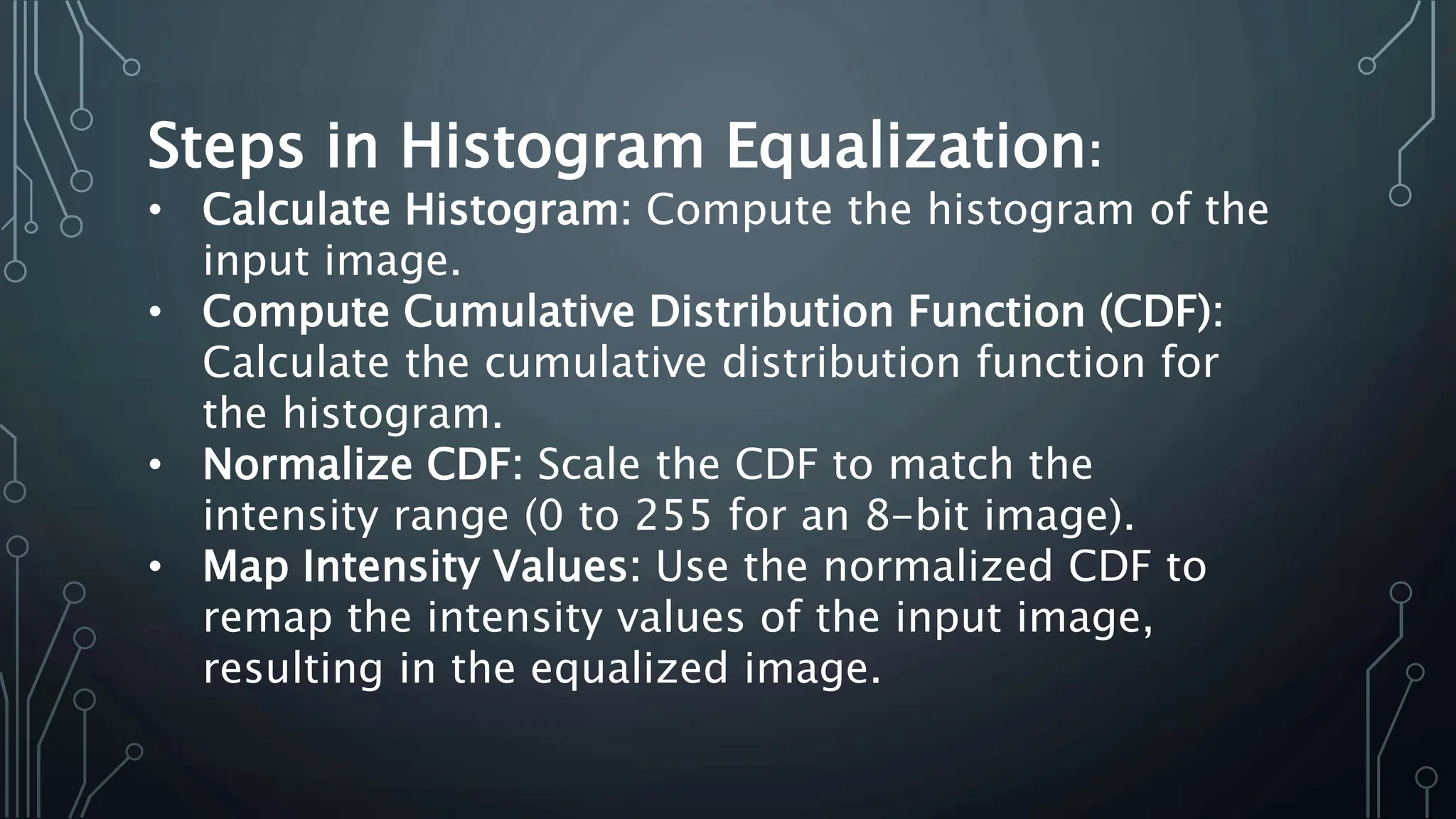
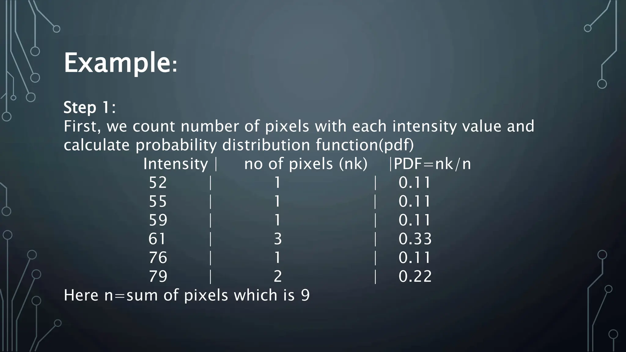
24. Example:
Consider this 3x3 grayscale image with intensity values
ranging from 0-255
Original Image:
[
[52, 55, 61],
[59, 79, 61],
[76, 61, 79]
]

25. Example:
Step 1:
First, we count number of pixels with each intensity value and
calculate probability distribution function(pdf)
Intensity | no of pixels (nk) |PDF=nk/n
52 | 1 | 0.11
55 | 1 | 0.11
59 | 1 | 0.11
61 | 3 | 0.33
76 | 1 | 0.11
79 | 2 | 0.22
Here n=sum of pixels which is 9

26. Example:
Step 2: Compute the Cumulative Distribution Function (CDF)
Next, we calculate the cumulative sum of the
histogram values:
Intensity | nk | PDF |CDF
52 | 1 | 0.11 |0.11
55 | 1 | 0.11 | 0.22
59 | 1 | 0.11 |0.33
61 | 3 | 0.33 |0.66
76 | 1 | 0.11 |0.77
79 | 2 | 0.22 |0.99

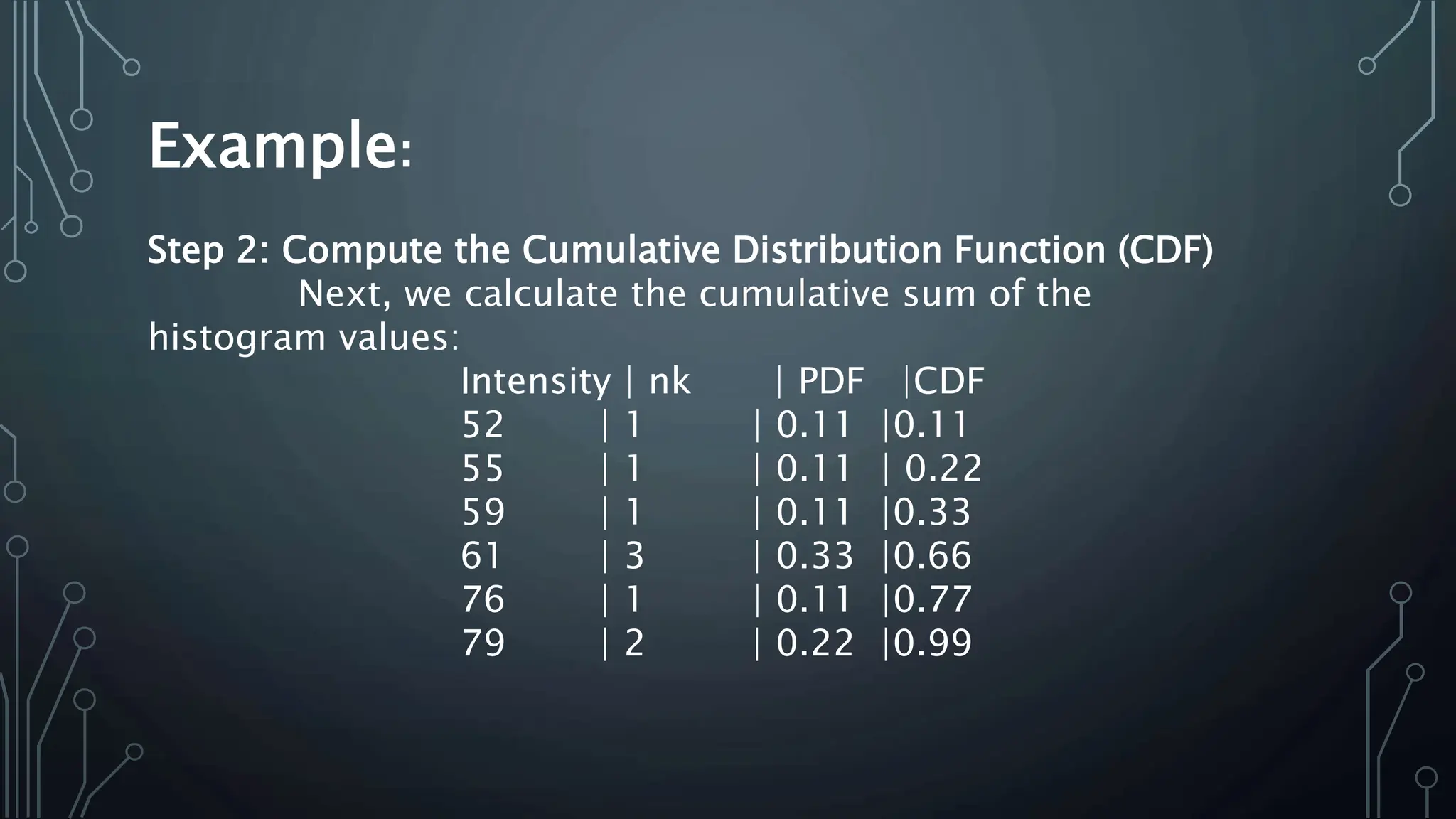
27. Example:
Step 3: Normalize the CDF
Normalize the CDF to the range [0, 255].
Intensity | nk | PDF |CDF |CDF X 255
52 | 1 | 0.11 |0.11 |28.05 ≈ 28
55 | 1 | 0.11 | 0.22 |56.1 ≈ 56
59 | 1 | 0.11 |0.33 |84.15 ≈84
61 | 3 | 0.33 |0.66 |168.3 ≈168
76 | 1 | 0.11 |0.77 |196.35 ≈ 196
79 | 2 | 0.22 |0.99 |252.45 ≈ 253

28. Example:
Step 4: Map the Intensity Values
Original | Equalized
52 | 28
55 | 32
59 | 56
61 | 168
76 | 196
79 | 253
SO
input image is
[
[52, 55, 61],
[59, 79, 61],
[76, 61, 79]
]
output image is
[
[28, 32, 168],
[56, 253, 168],
[196, 168, 253]
]

29. Properties:
Histograms clustered at
the low end correspond
to dark images.
Histograms clustered at
the high end correspond
to bright images.

30. Properties:
Histograms with small spread
correspond to low contrast images
(i.e., mostly dark, mostly bright, or
mostly gray).
Histograms with wide
spread correspond to high
contrast images.

31. Applications and Future Trends:
• Artificial Intelligence and Deep Learning
• Real-Time Processing
• High Dynamic Range (HDR) Imaging
• Adaptive and Context-Aware Enhancement
• Super-Resolution Imaging
• Integration with Augmented Reality (AR) and Virtual Reality
(VR)
• Ethical and Responsible Enhancement

32. THANKYO
U!