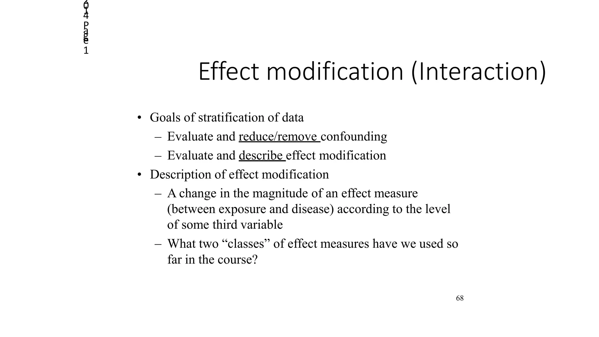
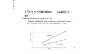
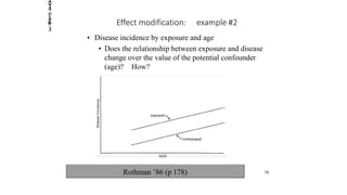
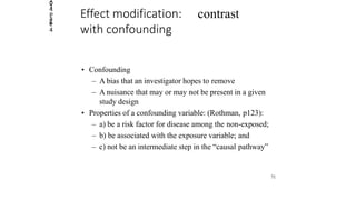
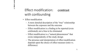
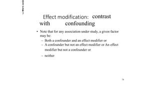
This document discusses effect modification and how it differs from confounding. It defines effect modification as a change in the magnitude of the effect of an exposure on an outcome according to levels of a third variable. Effect modification provides a more detailed description of the relationship between exposure and outcome, whereas confounding is a bias to be eliminated. The document contrasts effect modification and confounding, and provides examples to illustrate the concepts. It also discusses testing for effect modification using tests of homogeneity and how the interpretation of effect modification depends on the choice of effect measure.
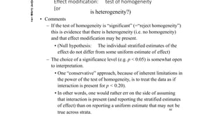
Bias, confounding and causality in p'coepidemiological researchsamthamby79
A brief description of three issues (Bias, Confounding and Causality) commonly encountered while performing pharmacoepidemiological research. A big THANK YOU to Mr. Strom and Mr. Kimmel.
Bias, confounding and causality in p'coepidemiological researchsamthamby79
A brief description of three issues (Bias, Confounding and Causality) commonly encountered while performing pharmacoepidemiological research. A big THANK YOU to Mr. Strom and Mr. Kimmel.
These annotated slides will help you interpret an OR or RR in clinical terms. Please download these slides and view them in PowerPoint so you can view the annotations describing each slide.
Declaration: The materials incorporated in this document have come from variety of sources and compiler bears no responsibilities for any information contained herein. The compiler acknowledges all the sources although references have not been explicitly cited for all the contents in this document.
Multiple Linear Regression II and ANOVA IJames Neill
Explains advanced use of multiple linear regression, including residuals, interactions and analysis of change, then introduces the principles of ANOVA starting with explanation of t-tests.
correlation or dependence is any statistical relationship, whether causal or not, between two random variables or bivariate data. Although in the broadest sense, "correlation" may indicate any type of association, in statistics it normally refers to the degree to which a pair of variables are linearly related. Familiar examples of dependent phenomena include the correlation between the height of parents and their offspring, and the correlation between the price of a good and the quantity the consumers are willing to purchase, as it is depicted in the so-called demand curve.
Correlations are useful because they can indicate a predictive relationship that can be exploited in practice. For example, an electrical utility may produce less power on a mild day based on the correlation between electricity demand and weather. In this example, there is a causal relationship, because extreme weather causes people to use more electricity for heating or cooling. However, in general, the presence of a correlation is not sufficient to infer the presence of a causal relationship (i.e., correlation does not imply causation).
Formally, random variables are dependent if they do not satisfy a mathematical property of probabilistic independence. In informal parlance, correlation is synonymous with dependence. However, when used in a technical sense, correlation refers to any of several specific types of mathematical operations between the tested variables and their respective expected values. Essentially, correlation is the measure of how two or more variables are related to one another. There are several correlation coefficients, often denoted
ρ
\rho or
r
r, measuring the degree of correlation. The most common of these is the Pearson correlation coefficient, which is sensitive only to a linear relationship between two variables (which may be present even when one variable is a nonlinear function of the other). Other correlation coefficients – such as Spearman's rank correlation – have been developed to be more robust than Pearson's, that is, more sensitive to nonlinear relationships.[1][2][3] Mutual information can also be applied to measure dependence between two variables.
BUS 308 Week 5 Lecture 3 A Different View Effect Sizes .docxcurwenmichaela
BUS 308 Week 5 Lecture 3
A Different View: Effect Sizes
Expected Outcomes
After reading this lecture, the student should be familiar with:
1. What effect size measures exist for different statistical tests.
2. How to interpret an effect size measure.
3. How to calculate an effect size measure for different tests.
Overview
While confidence intervals can give us a sense of how much variation is in our decisions,
effect size measures help us understand the practical significance of our decision to reject the
null hypothesis. Not all statistically significant results are of the same importance in decision
making. A difference in means of 25 cents is more important with means around a dollar than
with means in the millions of dollars, yet with the right sample size both groups can have this
difference be statistically significant.
Effect size measures help us understand the practice importance of our decision to reject
the null hypothesis.
Excel has limited functions available for us to use on Effect Size measures. We generally
need to take the output from the other functions and generate our Effect Size values.
Effect Sizes
One issue many have with statistical significance is the influence of sample size on the
decision to reject the null hypothesis. If the average difference in preference for a soft drink was
found to be ½ of 1%; most of us would not expect this to be statistically significant. And,
indeed, with typical sample sizes (even up to 100), a statistical test is unlikely to find any
significant difference. However, if the sample size were much larger; for example, 100,000; we
would suddenly find this miniscule difference to be significant!
Statistical significance is not the same as practical significance. If for example, our
sample of 100,000 was 1% more in favor of an expensive product change, would it really be
worthwhile making the change? Regardless of how large the sample was, it does not seem
reasonable to base a business decision on such a small difference.
Enter the idea of Effect Size. The name is descriptive but at the same time not very
illuminating on what this measure does. We will get to specific measures shortly, but for now,
let’s look at how an Effect Size measure can help us understand our findings. First, the name:
Effect Size. What effect? What size? In very general terms, the effect we are monitoring is the
effect that occurs when we change one of the variables. For example, is there an effect on the
average compa-ratio when we change from male to female. Certainly, but not all that much, as
we found no significant difference between the average male and female compa-ratios. Is there
an effect when we change from male to female on the average salary? Definitely. And it is
much larger than what we observed on the compa-ratio means. We found a significant
difference in the average salary for males than females – around $14,000.
The Effect Siz.
Overview of Multivariate Statistical MethodsThomasUttaro1
This is an overview of advanced multivariate statistical methods which have become very relevant in many domains over the last few decades. These methods are powerful and can exploit the massive datasets implemented today in meaningful ways. Typically analytics platforms do not deploy these statistical methods, in favor of straightforward metrics and machine learning, and thus they are often overlooked. Additional references are available as documented.
Model Attribute Check Company Auto PropertyCeline George
In Odoo, the multi-company feature allows you to manage multiple companies within a single Odoo database instance. Each company can have its own configurations while still sharing common resources such as products, customers, and suppliers.
Operation “Blue Star” is the only event in the history of Independent India where the state went into war with its own people. Even after about 40 years it is not clear if it was culmination of states anger over people of the region, a political game of power or start of dictatorial chapter in the democratic setup.
The people of Punjab felt alienated from main stream due to denial of their just demands during a long democratic struggle since independence. As it happen all over the word, it led to militant struggle with great loss of lives of military, police and civilian personnel. Killing of Indira Gandhi and massacre of innocent Sikhs in Delhi and other India cities was also associated with this movement.
Embracing GenAI - A Strategic ImperativePeter Windle
Artificial Intelligence (AI) technologies such as Generative AI, Image Generators and Large Language Models have had a dramatic impact on teaching, learning and assessment over the past 18 months. The most immediate threat AI posed was to Academic Integrity with Higher Education Institutes (HEIs) focusing their efforts on combating the use of GenAI in assessment. Guidelines were developed for staff and students, policies put in place too. Innovative educators have forged paths in the use of Generative AI for teaching, learning and assessments leading to pockets of transformation springing up across HEIs, often with little or no top-down guidance, support or direction.
This Gasta posits a strategic approach to integrating AI into HEIs to prepare staff, students and the curriculum for an evolving world and workplace. We will highlight the advantages of working with these technologies beyond the realm of teaching, learning and assessment by considering prompt engineering skills, industry impact, curriculum changes, and the need for staff upskilling. In contrast, not engaging strategically with Generative AI poses risks, including falling behind peers, missed opportunities and failing to ensure our graduates remain employable. The rapid evolution of AI technologies necessitates a proactive and strategic approach if we are to remain relevant.
June 3, 2024 Anti-Semitism Letter Sent to MIT President Kornbluth and MIT Cor...Levi Shapiro
Letter from the Congress of the United States regarding Anti-Semitism sent June 3rd to MIT President Sally Kornbluth, MIT Corp Chair, Mark Gorenberg
Dear Dr. Kornbluth and Mr. Gorenberg,
The US House of Representatives is deeply concerned by ongoing and pervasive acts of antisemitic
harassment and intimidation at the Massachusetts Institute of Technology (MIT). Failing to act decisively to ensure a safe learning environment for all students would be a grave dereliction of your responsibilities as President of MIT and Chair of the MIT Corporation.
This Congress will not stand idly by and allow an environment hostile to Jewish students to persist. The House believes that your institution is in violation of Title VI of the Civil Rights Act, and the inability or
unwillingness to rectify this violation through action requires accountability.
Postsecondary education is a unique opportunity for students to learn and have their ideas and beliefs challenged. However, universities receiving hundreds of millions of federal funds annually have denied
students that opportunity and have been hijacked to become venues for the promotion of terrorism, antisemitic harassment and intimidation, unlawful encampments, and in some cases, assaults and riots.
The House of Representatives will not countenance the use of federal funds to indoctrinate students into hateful, antisemitic, anti-American supporters of terrorism. Investigations into campus antisemitism by the Committee on Education and the Workforce and the Committee on Ways and Means have been expanded into a Congress-wide probe across all relevant jurisdictions to address this national crisis. The undersigned Committees will conduct oversight into the use of federal funds at MIT and its learning environment under authorities granted to each Committee.
• The Committee on Education and the Workforce has been investigating your institution since December 7, 2023. The Committee has broad jurisdiction over postsecondary education, including its compliance with Title VI of the Civil Rights Act, campus safety concerns over disruptions to the learning environment, and the awarding of federal student aid under the Higher Education Act.
• The Committee on Oversight and Accountability is investigating the sources of funding and other support flowing to groups espousing pro-Hamas propaganda and engaged in antisemitic harassment and intimidation of students. The Committee on Oversight and Accountability is the principal oversight committee of the US House of Representatives and has broad authority to investigate “any matter” at “any time” under House Rule X.
• The Committee on Ways and Means has been investigating several universities since November 15, 2023, when the Committee held a hearing entitled From Ivory Towers to Dark Corners: Investigating the Nexus Between Antisemitism, Tax-Exempt Universities, and Terror Financing. The Committee followed the hearing with letters to those institutions on January 10, 202
How to Make a Field invisible in Odoo 17Celine George
It is possible to hide or invisible some fields in odoo. Commonly using “invisible” attribute in the field definition to invisible the fields. This slide will show how to make a field invisible in odoo 17.
Exploiting Artificial Intelligence for Empowering Researchers and Faculty, In...Dr. Vinod Kumar Kanvaria
Exploiting Artificial Intelligence for Empowering Researchers and Faculty,
International FDP on Fundamentals of Research in Social Sciences
at Integral University, Lucknow, 06.06.2024
By Dr. Vinod Kumar Kanvaria
Acetabularia Information For Class 9 .docxvaibhavrinwa19
Acetabularia acetabulum is a single-celled green alga that in its vegetative state is morphologically differentiated into a basal rhizoid and an axially elongated stalk, which bears whorls of branching hairs. The single diploid nucleus resides in the rhizoid.
Macroeconomics- Movie Location
This will be used as part of your Personal Professional Portfolio once graded.
Objective:
Prepare a presentation or a paper using research, basic comparative analysis, data organization and application of economic information. You will make an informed assessment of an economic climate outside of the United States to accomplish an entertainment industry objective.
1. 2014
Page
1
68
Effect modification (Interaction)
• Goals of stratification of data
– Evaluate and reduce/remove confounding
– Evaluate and describe effect modification
• Description of effect modification
– A change in the magnitude of an effect measure
(between exposure and disease) according to the level
of some third variable
– What two “classes” of effect measures have we used so
far in the course?
2. exampleEffect modification:
#1
• Disease incidence by exposure and age
– Does the relationship between exposure and disease change
over the value of the potential confounder (age)? How?
69
2014
Page
2
3. Effect modification: example #2
• Disease incidence by exposure and age
• Does the relationship between exposure and disease
change over the value of the potential confounder
(age)? How?
Rothman ’86 (p 178)
2014
Page
3
70
4. 2014
Page
4
contrastEffect modification:
with confounding
• Confounding
– A bias that an investigator hopes to remove
– A nuisance that may or may not be present in a given
study design
• Properties of a confounding variable: (Rothman, p123):
– a) be a risk factor for disease among the non-exposed;
– b) be associated with the exposure variable; and
– c) not be an intermediate step in the “causal pathway”
71
5. 2014
Page
5
contrastEffect modification:
with confounding
• Effect modification
– A more detailed description of the “true” relationship
between the exposure and the outcome
– Effect modification is a finding to be reported (even
celebrated), not a bias to be eliminated
– Effect modification is a “natural phenomenon” that
exists independently of the study design
– The presence and interpretation of effect modification
depends upon the choice of effect measure (ratio vs.
difference)
72
7. 2014
Page
7
Effect modification: contrast
with confounding
• Note that for any association under study, a given factor
may be:
– Both a confounder and an effect modifier or
– A confounder but not an effect modifier or An effect
modifier but not a confounder or
– neither
74
10. Effect modification: test of
homogeneity
• Null hypothesis: The individual stratified estimates of the effect do not
differ from some uniform estimate of effect (such as a Mantel Haenszel
estimator)
• Notation:
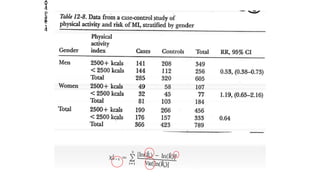
– N is the number of strata (N=2 in our smoking/matches example);
–
MH
ln^Ri is the natural logarithm of the estimated (hence the “^”) effect
measure for each stratum (ORi in our example);
– ln^R is the natural logarithm of the uniform effect estimate (e.g. OR in
– X2
(N-1)
is chi-square with (N-1) degrees of freedom;
our example—the computer will use the maximum likelihood estimate)
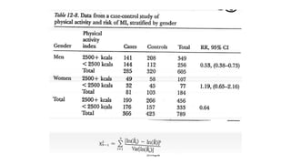
• One formula to test homogeneity:
X2
(N-1)
= ∑ [ln(^ Ri) – ln(RMH)]2
Var[ln(^
Ri)]
N
i= 1
78
JC: Comment on choice of signifciance level for test of homogeneity
2014
Page
10
11. 2014
Page
11
Paradox
• If effect modification is present, a uniform estimator of
effect (such as ORMH) cannot (or at least should not) be
reported.
• However, in order to determine if effect modification is
present, it is necessary to calculate the value of a uniform
estimator of effect (such as ORMH) because it is needed in
the calculation of the test of homogeneity.
79
12. 2014
Page
12
Effect modification: test of homogeneity
(or
is heterogeneity?)
• Comments
– If the test of homogeneity is “significant” (=“reject homogeneity”)
this is evidence that there is heterogeneity (i.e. no homogeneity)
and that effect modification may be present.
• (Null hypothesis: The individual stratified estimates of the
effect do not differ from some uniform estimate of effect)
– The choice of a significance level (e.g. p < 0.05) is somewhat open
to interpretation.
• One “conservative” approach, because of inherent limitations in
the power of the test of homogeneity, is to treat the data as if
interaction is present for p < 0.20).
• In other words, one would rather err on the side of assuming
that interaction is present (and reporting the stratified estimates
of effect) than on reporting a uniform estimate that may not be
true across strata.
80
15. Additive versus multiplicative scale effect modification
● Notation: RXZ
● No additive interaction if (R11 – R01) = (R10 – R00)
○ Rewrite as: (R11-R01)-(R10-R00)=0
● In words: Difference in risk for (X=1 vs. X=0) when Z=1 is
equal to difference in risk for (X=1 vs. X=0) when Z=0
● Note: the values R11, R10, etc. are risks (not counts)
2014
Page
15
16. Additive versus multiplicative scale effect modification
● Notation: RXZ
● No multiplicative interaction if (R11/R01)=(R10/R00)
Rewrite as: (R11/R01)/(R10/R00)=1
● In words: Ratio of risks/rates when X=1 vs. X=0 when
Z=1 is equal to ratio of risks/rates when X=1 vs. X=0
when Z=0
2014
Page
16
17. 2014
Page
17 Effect modification is scale-dependent
•Evidence for effect modification/statistical interaction
if the RR or the AR differs between two groups
•However, effect modification/statistical interaction is
scale-dependent
–If you do not have interaction on the additive scale (AR is
homogenous) then you will have interaction on the multiplicative
scale (RR must be heterogeneous)
–If you do not have interaction on the multiplicative scale (RR is
homogenous) then you will have interaction on the additive scale
(AR must be heterogeneous)
–Note: It is common to have evidence of interaction on both
scales.
18. Example
● No additive scale interaction if (R11-R01)-(R10-R00)=0
● No relative scale interaction if (R11/R01)/(R10/R00)=1
● Additive scale: (60-20) - (50-10) = 0
○ Interaction not present on the additive scale
● Relative scale: (60/20) / (50/10)=0.6
○ Interaction present on the relative scale
Z=1 Z=0
X=1 60 50
X=0 20 10
2014
Page
18
19. Example
● No additive scale interaction if (R11-R01)-(R10-R00)=0
● No relative scale interaction if (R11/R01)/(R10/R00)=1
● Additive scale: (60-20) - (30-10) = 20
○ Interaction present on the additive scale
● Relative scale: (60/20) / (30/10)=1
○ Interaction not present on the relative scale
Z=1 Z=0
X=1 60 30
X=0 20 10
2014 Page 100