The document discusses the differences and relationships between quadratic functions and quadratic equations. It notes that quadratic functions can take any real number as an input, while quadratic equations only have two solutions. The roots of a quadratic equation are also the x-intercepts of the graph of the corresponding quadratic function. The remainder theorem states that the value of a polynomial when a number is substituted for the variable is equal to the remainder when the polynomial is divided by the linear factor corresponding to that number. This connects the roots of quadratic equations to factors of quadratic functions. A quadratic can only have two distinct roots, as having three would mean it has an infinite number of roots.

1. QUADRATIC FUNCTIONS
The equation 𝑓(𝑥) = 𝑦 = 𝑎𝑥2
+ 𝑏𝑥 + 𝑐………………..(A)
Is called quadratic function. What is the difference between the
quadratic equation 𝑎𝑥2
+ 𝑏𝑥 + 𝑐 = 0 and the quadratic function
𝑓(𝑥) = 𝑦 = 𝑎𝑥2
+ 𝑏𝑥 + 𝑐 ? The quadratic equation (A) is valid
for only two values of the variable x, the two roots of the equation 𝛼, 𝛽
for which the value of the expression is 0. But for other values of x,
𝑓(𝑥) = 𝑦 ≠ 0.The independent variable x can take any value from
-∞ to ∞ in this case. The interval ] − ∞, ∞[ is called domain of the
function and the range (or codomain of function) is the set of values y
can take, which depends upon the coefficients a, b and c; here it is a
smaller set ,not interval ] − ∞, ∞[ . Obviously the roots 𝛼, 𝛽 depend
upon the coefficients and vice versa.
We could write the above quadratic function like
𝑎𝑥2
+ 𝑏𝑥 + (𝑐 − 𝑦) = 0,or, 𝑎𝑥2
+ 𝑏𝑥 + 𝐶 = 0,where
𝐶 = 𝑐 − 𝑦; so that for each value of the dependent variable 𝒚 the
quadratic function is a new quadratic equation.
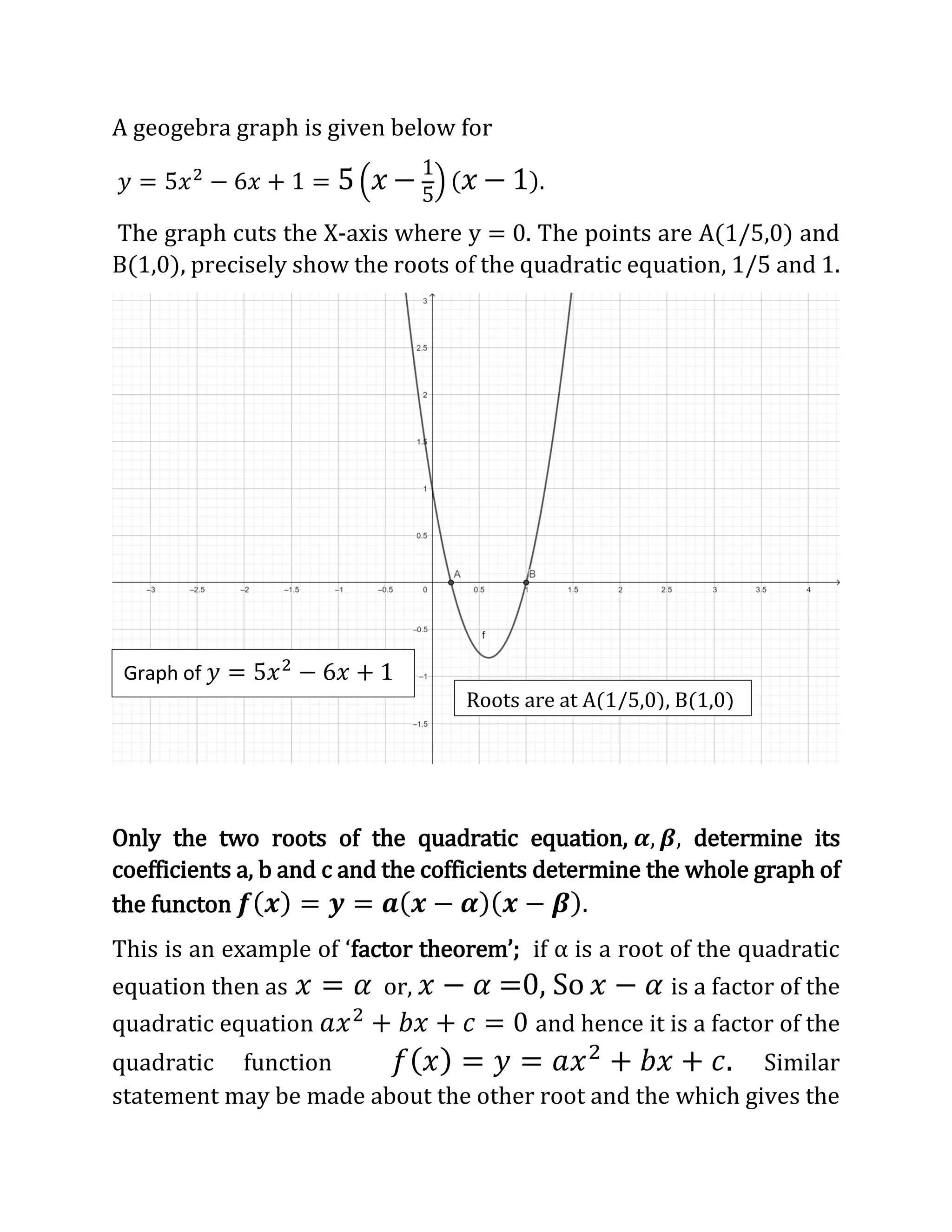
For a particular set of values of a, b and c ( say 5, – 6 and 1 for
example) we can write 𝑓(𝑥) = 𝑦 = 𝑎(𝑥 − 𝛼)(𝑥 − 𝛽)……..(B)
(in the particular case 𝑓(𝑥) = 𝑦 = 5 (𝑥 −
1
5
) (𝑥 − 1)).
The graph of quadratic function is a “curve” in the x-y Cartesian plane
whereas the quadratic equation stands for only two points in the
plane (𝛼, 0) and (𝛽, 0), when we put 𝑦 = 0 in the quadratic function.
These two points are the points where the graph of the quadratic
function cuts the X-axis (interception of the curve with X-axis).

2. A geogebra graph is given below for
𝑦 = 5𝑥2
− 6𝑥 + 1 = 5(𝑥 − 1
5
) (𝑥 − 1).
The graph cuts the X-axis where y = 0. The points are A(1/5,0) and
B(1,0), precisely show the roots of the quadratic equation, 1/5 and 1.
Only the two roots of the quadratic equation, 𝜶, 𝜷, determine its
coefficients a, b and c and the cofficients determine the whole graph of
the functon 𝒇(𝒙) = 𝒚 = 𝒂(𝒙 − 𝜶)(𝒙 − 𝜷).
This is an example of ‘factor theorem’; if α is a root of the quadratic
equation then as 𝑥 = 𝛼 or, 𝑥 − 𝛼 =0, So 𝑥 − 𝛼 is a factor of the
quadratic equation 𝑎𝑥2
+ 𝑏𝑥 + 𝑐 = 0 and hence it is a factor of the
quadratic function 𝑓(𝑥) = 𝑦 = 𝑎𝑥2
+ 𝑏𝑥 + 𝑐. Similar
statement may be made about the other root and the which gives the
Graph of 𝑦 = 5𝑥2
− 6𝑥 + 1
Roots are at A(1/5,0), B(1,0)

3. other factor. The fact shall be further clarified from ‘remainder
theorem’.
The remainder theorem (Euclidean polynomial remainder theorem)
says that if a polynomial function 𝑓(𝑥) is divided by a linear
polynomial −𝑟 , the remainder is 𝑓(𝑟); i.e., the function value when x
is replaced by r. Not only quadratic polynomials, this is valid for
polynomials of any positive integer degree. Observe the following:
𝑓(𝑥)
𝑥 − 𝑟
=
𝑎𝑥2
+ 𝑏𝑥 + 𝑐
𝑥 − 𝑟
=
𝑎𝑥2
− 𝑎𝑟𝑥 + 𝑎𝑟𝑥 + 𝑏𝑥 + 𝑐
𝑥 − 𝑟
=
𝑎𝑥(𝑥−𝑟)+𝑥(𝑏+𝑎𝑟)+𝑐
𝑥−𝑟
= 𝑎𝑥 +
(𝑥−𝑟)(𝑏+𝑎𝑟)+𝑟(𝑏+𝑎𝑟)+𝑐
𝑥−𝑟
=𝑎𝑥 + 𝑏 + 𝑎𝑟 +
𝑎𝑟2+𝑏𝑟+𝑐
𝑥−𝑟
= 𝑎𝑥 + 𝑏 + 𝑎𝑟 +
𝑓(𝑟)
𝑥−𝑟
Evidently 𝑎𝑟2
+ 𝑏𝑟 + 𝑐 = 𝑓(𝑟), is the value of 𝒇(𝒙) when x is
replaced by r. And 𝑎𝑟2
+ 𝑏𝑟 + 𝑐 = 𝑓(𝑟), is also the remainder
when 𝑓(𝑥) is divided by 𝑥 − 𝑟. The things will be more vivid if 𝑎𝑥2
+
𝑏𝑥 + 𝑐 is divided by 𝑥 − 𝑟 in long division process. This is not only
true of quadratic polynomials but all polynomials of higher integer
degrees.
Let 𝑓(𝑥) be a polynomial of any integer higher degree. Let the
quotient be 𝑄(𝑥) when it is divided by 𝑥 − 𝑟 and R be the remainder.
We can write 𝒇(𝒙) = 𝑸(𝒙)(𝒙 − 𝒓) + 𝑹. This is division algorithm.

4. The general statement of the division algorithm is
Let 𝑓(𝑥) be a polynomial of any integer higher degree. Let the
quotient be 𝑄(𝑥) when it is divided by 𝑔(𝑥), where degree of 𝑔(𝑥) is
less than degree of 𝑓(𝑥) and 𝑅(𝑥) be the remainder and degree
of 𝑅(𝑥) is less than that of 𝑔(𝑥) . We can write 𝒇(𝒙) = 𝑸(𝒙)𝒈(𝒙) +
𝑹(𝒙).
If 𝑔(𝑥) divides (𝑥) , we et get 𝑓(𝑟) = 𝑄(𝑟). 0 + 𝑅
The factor theorem reduces to be a particular case of the remainder
theorem; 𝑓(𝑥) = 0 if 𝑥 = 𝑟 and in any quadratic equation.
This finally explains the difference and similarity between the
quadratic function and quadratic equation. We can calculate the value
of say𝑓(3), for 𝑥 = 3 without any tedious calculation or without
undertaking the actual long division process.
This would be 𝑓(3) = 𝑎. 32
+ 𝑏. 3 + 𝑐 without actually calculating
it.
Roots of the quadratic function or quadratic equation
The roots 𝛼, 𝛽 of the quadratic equation 𝑎𝑥2
+ 𝑏𝑥 + 𝑐 = 0 are also
called the roots of the quadratic function 𝑦 = 𝑓(𝑥) = 𝑎𝑥2
+ 𝑏𝑥 + 𝑐.
As per Fundamental theorem of algebra every polynomial equation
has a root.
If 𝛼 is a root of 𝑓(𝑥) = 𝑎𝑥2
+ 𝑏𝑥 + 𝑐, then 𝑥 − 𝛼 is a factor of the
function 𝑓(𝑥) = 𝑎𝑥2
+ 𝑏𝑥 + 𝑐. Now divide this by 𝑥 − 𝛼 by long

5. division process and get 𝑓(𝑥) = (𝑎𝑥 + 𝑎𝛼 + 𝑏)(𝑥 − 𝛼) + 𝑅 , where
𝑓(𝛼) = 𝑅 = 0 by remainder theorem, putting 𝑥 = 𝛼 throughout.
Then 𝑓(𝑥) = (𝑎𝑥 + 𝑎𝛼 + 𝑏)(𝑥 − 𝛼), which is also 0
when 𝑎𝑥 + 𝑎𝛼 + 𝑏 = 0. This gives 𝑥 − (−𝛼 −
𝑏
𝑎
) = 0.
Thus −𝛼 −
𝑏
𝑎
is another root of the function 𝑓(𝑥) = 𝑎𝑥2
+ 𝑏𝑥 + 𝑐.
So, observe that −𝛼 −
𝑏
𝑎
= 𝛽, the other root of the equation the
quadratic equation must have two roots, for 𝛼 + 𝛽 = −
𝑏
𝑎
, as we
already know. In some special case to be discussed later, both the
roots may be equal or coincident. In this way it could be shown that
a polynomial equation of degree n shall have n roots i.e. it may be
decomposed into product of n linear factors
What the fundamental theorem of algebra means is this. We may
multiply any two factors 𝑥 − 𝛼, and 𝑥 − 𝛽 for any two arbitrary
numbers 𝛼 and 𝛽 and their product
(𝑥 − 𝛼)(𝑥 − 𝛽) = 𝑥2
− (𝛼 + 𝛽)𝑥 + 𝛼𝛽 is a quadratic expression.
Fundamental theorem of algebra tells us just the reverse. Given any
quadratic expression 𝑝𝑥2
+ 𝑞𝑥 + 𝑟, p, q, r being numbers
whatsoever, this expression can be expressed as multiplication of
two linear 𝒙 − 𝜸 and 𝒙 − 𝜹such as 𝒂(𝒙 − 𝜸)(𝒙 − 𝜹), but the
theorem does not tell us anything about how these factors may be
found out, nor the theorem tells us about the nature of these roots;
what kinds of numbers they may be. This theorem was first proved
by Gauss three times in his life time in different ways, although it
was known much earlier. This is one of the important proofs of the
millennium.

6. In this manner we may show that a polynomial of degree n must
have at least one root, by fundamental theorem of algebra, and
eventually must have n roots, whether distinct or not.
We doubly emphasize this point, a quadratic equation cannot have
more than two distinct roots, and in the same vein, a polynomial of
degree n cannot have more than n distinct roots. If not, see the
consequence.
If possible, let the quadratic equation 𝑎𝑥2
+ 𝑏𝑥 + 𝑐 = 0 have 3
distinct roots, 𝛼, 𝛽, 𝛾 such that 𝛼 ≠ 𝛽 ≠ 𝛾. So we have,
𝑎𝛼2
+ 𝑏𝛼 + 𝑐 = 0………………………………..(a)
𝑎𝛽2
+ 𝑏𝛽 + 𝑐 = 0………………………………..(b)
𝑎𝛾2
+ 𝑏𝛾 + 𝑐 = 0………………………………..(c)
Subtracting (b) from (a), 𝑎(𝛼2
− 𝛽2) + 𝑏(𝛼 − 𝛽) = 0
Or, (𝛼 − 𝛽)(𝑎𝛼 + 𝑎𝛽 + 𝑏) = 0
Or, 𝑎𝛼 + 𝑎𝛽 + 𝑏 = 0 since 𝛼 ≠ 𝛽…………………(d)
Subtracting (c) from (a), 𝑎(𝛼2
− 𝛾2) + 𝑏(𝛼 − 𝛾) = 0
In the same way we get 𝑎𝛼 + 𝑎𝛾 + 𝑏 = 0 since 𝛼 ≠ 𝛾………(e)
Subtracting (e) from (d), we get, 𝑎(𝛽 − 𝛾) = 0………………..(f)
If 𝛽 ≠ 𝛾, we have to accept that a = 0, Similarly we can show that b
=0 and c = 0. Thus 𝑎𝑥2
+ 𝑏𝑥 + 𝑐 = 0 becomes 0.𝑥2
+ 0𝑥 + 0 = 0,
which is no more a quadratic equation, even it is not an equation. It
is true for any value of x, 𝛼, 𝛽, 𝛾, 𝛿, 𝜀, …, anything . We call this is an
identity, which is true for every value of the variable. In other words,
if a quadratic equation has three distinct roots, it has infinite
number of different roots.

7. Example 1
Show that
𝑎2−𝑥2
(𝑎−𝑏)(𝑎−𝑐)
+
𝑏2−𝑥2
(𝑏−𝑐)(𝑏−𝑎)
+
𝑐2−𝑥2
(𝑐−𝑎)(𝑐−𝑏)
− 1 = 0 is
an identity.
Solution:, Put x = a in the expression and see that it reduces to 0. So
a is a root of the equation. Similarly show that b and c are also roots
of the equation. Since we have not assumed 𝑎 = 𝑏 = 𝑐, they are
different from each other and the quadratic equation has 3 different
roots. So it must be identically 0.
Example 2
Show that
𝑎2(𝑥−𝑏)(𝑥−𝑐)
(𝑎−𝑏)(𝑎−𝑐)
+
𝑏2(𝑥−𝑐)(𝑥−𝑎)
(𝑏−𝑐)(𝑏−𝑎)
+
𝑐2(𝑥−𝑎)(𝑥−𝑏)
(𝑐−𝑎)(𝑐−𝑏)
− 𝑥2
= 0 is an identity.
Solution:, Put x = a in the expression and see that it reduces to 0. So
a is a root of the equation. Similarly show that b and c are also roots
of the equation. Since we have not assumed 𝑎 = 𝑏 = 𝑐, they are
different from each other and the quadratic equation has 3 different
roots. So it must be identically 0.