Downloaded 39 times


![Parametric Curves
•Separate equation for each spatial variable
x=x(u)
y=y(u)
z=z(u)
• For umax ≥ u ≥ umin we trace out a curve in two or three
dimensions
9
p(u)=[x(u), y(u), z(u)]T
p(u)
p(umin)
p(umax)](https://image.slidesharecdn.com/ds3tu6or4ehnkpn5cmpn-signature-07c8814cc3b9b0aa65ed4e20d314240a678be73835f52dff908a264ad08c8a05-poli-170406094108/75/Curves-and-Surfaces-9-2048.jpg)


![Parametric Surfaces
• Surfaces require 2 parameters
x=x(u,v)
y=y(u,v)
z=z(u,v)
p(u,v) = [x(u,v), y(u,v), z(u,v)]T
• Want same properties as curves:
• Smoothness
• Differentiability
• Ease of evaluation
12
x
y
z p(u,0)
p(1,v)
p(0,v)
p(u,1)](https://image.slidesharecdn.com/ds3tu6or4ehnkpn5cmpn-signature-07c8814cc3b9b0aa65ed4e20d314240a678be73835f52dff908a264ad08c8a05-poli-170406094108/75/Curves-and-Surfaces-12-2048.jpg)


![Curve Segments
•After normalizing u, each curve is written
p(u)=[x(u), y(u), z(u)]T
, 1 ≥ u ≥ 0
•In classical numerical methods, we design a single
global curve
•In computer graphics and CAD, it is better to design
small connected curve segments
16
p(u)
q(u)
p(0)
q(1)
join point p(1) = q(0)](https://image.slidesharecdn.com/ds3tu6or4ehnkpn5cmpn-signature-07c8814cc3b9b0aa65ed4e20d314240a678be73835f52dff908a264ad08c8a05-poli-170406094108/75/Curves-and-Surfaces-16-2048.jpg)


![Cubic Polynomial Surfaces
20
vucvu ji
i j
ij∑∑= =
=
3
0
3
0
),(p
p(u,v)=[x(u,v), y(u,v), z(u,v)]T
where
p is any of x, y or z
Need 48 coefficients ( 3 independent sets of 16) to
determine a surface patch](https://image.slidesharecdn.com/ds3tu6or4ehnkpn5cmpn-signature-07c8814cc3b9b0aa65ed4e20d314240a678be73835f52dff908a264ad08c8a05-poli-170406094108/75/Curves-and-Surfaces-20-2048.jpg)

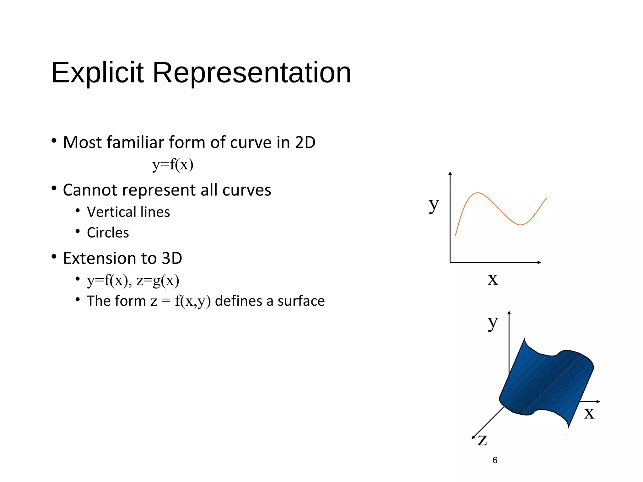
1. The document introduces different types of curves and surfaces including explicit, implicit, and parametric representations. It discusses their strengths and weaknesses. 2. Parametric curves and surfaces are presented as flexible representations that can approximate or interpolate data using functions that are smooth, differentiable, and easy to evaluate. 3. The document provides examples of parametric representations for lines, planes, spheres, and polynomial curves and surfaces. It emphasizes the importance of continuity between connected curve segments.