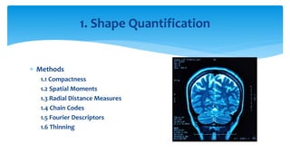
1. The document discusses various methods for quantifying two-dimensional shapes and textures in medical images, including statistical moments, spatial moments, radial distance measures, chain codes, Fourier descriptors, thinning, and texture measures. 2. Compactness, calculated using perimeter and area, quantifies how close a shape is to a circle. Spatial moments provide quantitative measurements of point distributions and shapes. Radial distance measures analyze boundary curvature. Chain codes represent boundary points. 3. Fourier descriptors and thinning/skeletonization reduce shapes to descriptors and graphs for analysis. Texture is quantified using statistical moments, co-occurrence matrices, spectral measures, and fractal dimensions.

1. Two-Dimensional Shape and Texture
Quantification
Medical Image Processing-BM4300
120405P
Shashika Chamod Munasingha

2.  Giving a numerical representation for a special attribute that maps the
human sense
 Ex: Let’s think of the shape circle. Radius/diameter is a quantitative value to
represent how big the circle is.
Quantification
r1
r2

3.  Methods
1.1 Compactness
1.2 Spatial Moments
1.3 Radial Distance Measures
1.4 Chain Codes
1.5 Fourier Descriptors
1.6 Thinning
1. Shape Quantification

4.  Computed using the perimeter (P) and the area (A) of the segmented region
 𝑪 = 𝑷 𝟐/𝑨
 Quantifies how close a shape is to the smoothest shape; circle
 When the C is getting larger for a particular shape, it moves away from the shape
circle.
 Perfect circle has the smallest value for C
 More details: ‘State of the Art of Compactness and Circularity Measures’ by Raul S. Montero
and Ernesto Bribiesca, 2009
1.1 Compactness (C)

5.  Calculating C
1.1 Compactness
𝐶 =
(2𝜋𝑟)2
𝜋𝑟2
𝐶 = 4𝜋
𝐶 = 12.57
r
a
a
𝐶 =?

6.  ITK Implementation
1.1 Compactness
 Region growing segmentation
 Shape attributes class
 Get the area and perimeter
 Calculate the compactness

7.  Advantages
 Invariant descriptor for
scale, rotation and
translation.
 Computational simplicity
 Often a good estimation
for shape roughness
1.1 Compactness
 Drawbacks
 Not always a robust
estimator of shape
complexity
C=15.4 C=27.6

8.  Quantitative measurement of the distribution and the shape of set of
points
 A 2D digital image can be represented by 3 parameters (i ,j ,f ) ;
 ( i , j ) spatial coordinates and f( i, j ) be the intensity of pixels
 More details : ‘Application of Shape Analysis to Mammographic Calcifications’ by Liang
Shen, Rangaraj M. Rangayyan, and J. E. Leo Desautels
1.2 Spatial Moments

9.  The first moments of a 2D image
 Infinite set of moment coefficients
 Can be retrieved the original image
 But not practical
 Finite set of moments can be used to retain useful information about the
image
 For binary images it quantifies the shape
 For gray scale images it quantifies the shape as well as the intensity
distribution
1.2 Spatial Moments

10.  Central moments
 Translation invariant
 Think of an image scaled by a factor of s (>1), the central moment will be
 How could we have a scale invariant descriptor?
 Scale down the image axes by a factor of µ00
( µ00
=area of the
object),then calculate the central moments or
 Direct calculation
1.2 Spatial Moments

11. What's more?
 Scale , translation and rotation invariant descriptor
 Orientation of a shape
 Eccentricity of a shape
1.2 Spatial Moments

12.  Results
1.2 Spatial Moments
X 2
Rotation
New : ‘Carotid artery image segmentation using modified spatial fuzzy c-means and ensemble clustering’, by Mehdi
Hassan ,Asmatullah Chaudhry, Asifullah Khan & Jin Young Kim (2012)

13.  Shape analyzing using its boundary ; variations and its curvature
Calculating the radial distance
 Let (x(n),y(n)) be the boundary pixel values
 (𝑥 𝑐 , 𝑦𝑐) = Centroid of the
segmented area
 The normalized radial distance(r(n)) can be obtained by dividing the d(n)
by the maximum d(n) value.
1.3 Radial Distance Measures

14.  The r(n) sequence can be used to obtain the statistical moments
First moments
Central moments
1.3 Radial Distance Measures

15.  Normalized moments
 Invariant to translation, rotation and scaling
 Important: The moment orders greater than 4 are not used as they are highly
sensitive to noise
1.3 Radial Distance Measures

16.  Results
1.3 Radial Distance Moments
X 2
Rotation

17. More..
 The features,
 Invariant as well as 𝑓21 = 𝑓2 − 𝑓1 monotonic increase with the shape complexity.
1.3 Radial Distance Measures

18.  The number of times the r(n) signal crosses the mean is a measurement of the
shape smoothness.
 The r(n) can also be analyzed in Fourier domain (spectral) .
 Coefficients with the highest value contain the essential shape information.
1.3 Radial Distance Measures
C
r(n)
1
N-1
n
r(n)
1
n

19.  Also a shape boundary measurement
 A shape can be quantified by the relative position of consecutive points in its
boundary
Method
 Each point in the boundary is assigned a label according to the relative position
from the previous point
 Clockwise or counter clockwise walking can be chosen
 4- connectivity or 8-connectivity base can be used
1.4 Chain Codes
3 2 1
4 P 0
5 6 7
1
2 P 0
3

20.  High resolution grid is not suitable in obtaining the chain codes
Why?
 Because high resolution means high sensitivity to noise as well
 Hence low resolution grid is imposed on the extracted boundary of the shape
1.4 Chain Codes
Tip like
structure is due
to the noise

21.  Example : 8-connected chain code in counter clockwise direction
What about the starting point (s) of the chain code?
When S changes the chain code will also be changed
Hence the chain code which gives the minimum value for the sum is considered to be chain code of that
shape .
1.4 Chain Codes
4 3
4 6 2
6 0 2 0
s 0
0 -> 2 ->0 ->2 ->3 ->4 ->6 ->4 ->6 ->0

22.  A rotation invariant code can be obtained using the first difference of the chain
code.
 Counter clockwise direction – Positive
 Clockwise direction – Negative
 Different for different boundaries, hence it can be used to distinguish different shapes.
 But cannot be used to compare the scale
1.4 Chain Codes
2, -2, 2, 1, 1, 2, -2, 2, -6

23. Is that all?
 If the differential chain code shows very small values (0,1) over a local section of
a boundary that section tends to be smoother.
 If the shape is symmetric or nearly symmetric, the differential chain code will
also have symmetric parts too.
 Concave and Convex regions can also be identified using differential chain code
 Continuous positive differences – Convex region
 Continuous negative differences – Concave region
New:
 ‘A measure of tortuosity based on chain coding’ by E Bribiesca - Pattern Recognition, 2013 – Elsevier
 ‘An automated lung segmentation approach using bidirectional chain codes to improve nodule detection
accuracy’ by S Shen, AAT Bui, J Cong, W Hsu - Computers in biology and medicine, 2015 - Elsevier
1.4 Chain Codes

24.  Each pixel on a selected contour can be represented by a complex number.
 The DFT
 Inverse DFT
 Except the first coefficient d(0) in DFT (centroid), all other coefficients are translation
invariant
 Important information is on lower order coefficients of d(u)
1.5 Fourier Descriptors

25.  d(u) is dependent upon the starting point of pixel array
𝑑 𝑠=coefficients after moving the starting point by 𝑛 𝑠 pixels
 FT properties can be effectively used in obtaining invariant descriptors
 The rotation of the object by angle 𝜃, shift of the starting point and scale by a factor
of a yields the DFT series
1.5 Fourier Descriptors

26.  The starting point, translation, scale and rotation invariant descriptors can be
obtained with
 The magnitudes of the normalized descriptors are scale invariant
 The descriptor so call the ‘shape factor (FF)’ is invariant to all above , low
sensitive to noise and a good quantifier of shape complexity/roughness.
1.5 Fourier Descriptors

27. We have talked a lot about Fourier Descriptors. But,
 All the results are based on the assumption; equidistance between pixel values of the
contour
 Can be achieved by 4-connected pixels
 Then the diagonal orientations are over estimated.
 If the region is large enough equidistance points can be selected along the contour, not
necessarily be the adjacent pixels
New: ‘Thermography based breast cancer analysis using statistical features and fuzzy classification’ by
Gerald Schaefer
1.5 Fourier Descriptors

28.  The essential shape information can be represented by reducing the shape to a
graph(skeleton)
 Skeleton is made of the medial lines along the main shape
 Medial lines are obtained via the medial axis transformation (MAT).
 The computational complexity is high for the MAT algorithm.
 Some iterative algorithms are introduced to reduce the computational
complexity
 Algorithm by Zhang and Suen is the widely used one among them
1.6 Thinning/Skeleton

29. Zhang and Suen Algorithm
 Iterative method to remove the boundary pixels of a shape and obtain the
skeleton
 The segmented area/shape should be converted to binary image where inside
of the contour is black (value 1) and outside is white (value 0) or the inverse.
1.6 Thinning
0 1

30. Z & S algorithm conti..
 Talking about two sums
 Non –zero neighbor sum n(𝑝1)
 0 to 1 transitions sum s(𝑝1)
 Ex:
1.6 Thinning
n(𝑝1) = 4
s(𝑝1) = 2
Pixel labels

31. Z & S algorithm conti..
 Step 1 : Determining the boundary pixels
 1 valued pixel with at least a 0 valued neighbor pixel is a boundary pixel
 Step 2: Delete the pixel, if following 4 conditions are satisfied simultaneously
 Condition 1: 𝟐 ≤ 𝒏(𝒑 𝟏) ≤ 𝟔
if 𝑛(𝑝1) = 1 then the pixel is an end pixel
if 𝑛(𝑝1) = 7 then the deleting may split the region
1.6 Thinning
0 1 1
1 1 1
0 1 1
0 0 0
0 1 0
0 1 0

32. Z & S algorithm conti..
 Condition 2: s(𝒑 𝟏) = 1
 If more than 0 to 1 transitions ,deleting 𝒑 𝟏 may lead to split the region
 Condition 3: 𝒑 𝟐 ∗ 𝒑 𝟒 ∗ 𝒑 𝟔 = 𝟎
 Condition 4: 𝒑 𝟒 ∗ 𝒑 𝟔 ∗ 𝒑 𝟖 = 𝟎
 Mark 𝒑 𝟏for deletion (Do not delete!) -> Delete after evaluation of all the pixels
1.6 Thinning
𝒑 𝟔 = 0 or 𝒑 𝟒 = 𝟎 or 𝒑 𝟖 = 𝒑 𝟐 = 𝟎
𝒑 𝟒 = 𝟎
East border
𝒑 𝟔 = 0
South border
𝒑 𝟒 = 𝒑 𝟐 = 𝟎
Northwest corner

33.  Step 3 :Apply the step2, first two conditions along with the new two conditions to the
result of the step2
 Condition 3: 𝒑 𝟐 ∗ 𝒑 𝟒 ∗ 𝒑 𝟖 = 𝟎
 Condition 4: 𝒑 𝟐 ∗ 𝒑 𝟔 ∗ 𝒑 𝟖 = 𝟎
 These two conditions yield the north, west borders and the southeast corner in the similar
manner
 Mark for deletion
 Delete the marked after running the step 3 to all the boundary pixels
 Iteratively apply the step 2 to the results of step 3
 Iteration stops when no pixel is marked in both step 2 and step 3
1.6 Thinning
𝒑 𝟐 = 0 or 𝒑 𝟖 = 𝟎 or 𝒑 𝟒 = 𝒑 𝟔 = 𝟎

34. Results
1.6 Thinning
Small section of an image After applying the
thinning algorithm
New:
‘Human body and posture recognition system based on an improved thinning algorithm’ by F Xie, G Xu, Y Cheng, Y Tian –
IET image processing, 2011 - ieeexplore.ieee.org

35.  Texture –
 A regular repetition of an element or pattern on a surface. (‘Statistical Texture Analysis’
by G. N. Srinivasan, and Shobha G.)
 The nature of a surface as defined by the irregularities on the surface.
Methods
2.1 Statistical Moments
2.2 Co-Occurrence Matrix Measures
2.3 Spectral Measures
2.4 Fractal Dimensions
2.5 Run-length Statistics
2. Texture Quantification

36. Based on,
 The smooth region contains pixel value close to each other
 Where as a rough region has wide variation in pixel values
 Intensity histograms
Consider an image with K gray levels (0,K-1).
Region with histogram h(k)
mean value of 𝜇 =
ℎ 𝑘 .𝑘𝐾−1
𝑘=0
ℎ 𝑘𝐾−1
𝑘=0
2.1 Statistical Moments

37.  The nth moment about the mean is defined as
 The second moment 𝒎 𝟐 (variance) is an important texture measurement.
 It correlates with the visual roughness perception.
 But,
 The third and fourth moments, skewness (symmetric nature) and kurtosis (Peakedness)
respectively cannot be used as texture measurements.
 Because they do not always correlate with texture
 In special cases where their potential value is pre quantified we can use them as well.
2.1 Statistical Moments

38. 2.1 Statistical Moments
Ultrasonic image of normal liver(left) , fatty liver(middle) and cirrhosis(right)

39. Drawbacks
 No spatial information
 Hence may lost important information like grainy structure
What about the following images? (50% white and 50% black pixels)
2.1 Statistical Moments
New:
‘Breast tissue classification using statistical feature extraction of mammograms’ by HS Sheshadri, A Kandaswamy

40.  ‘Gray Level Co-Occurrence Matrix’ (GLCM)
 Co-Occurrence matrix
 Pair of pixels with specific values
 In specific orientation and distance
 How often they occur
 Quantification the texture by extracting the statistical measures from the GLCM
 Typical orientation values 𝟎 𝒐
, 𝟗𝟎 𝒐
, 𝟒𝟓 𝒐
𝒂𝒏𝒅 𝟏𝟑𝟓 𝒐
 Typical distance values 𝒅 = 𝟏 (0 𝑜, 90 𝑜) and 𝒅 = 𝟐(45 𝑜, 135 𝑜)
2.2 C0-Occurrence Matrix Measures

41. Ex: Consider an image of 6x6=36 pixels (P) and 4 gray levels(K) (0,1,2 and 3)
 The matrix of 4x4 (based on gray levels) which contains count for specific d and 𝜽 H(d, 𝜽)
H( 𝟐, 𝟒𝟓 𝒐
)
2.2 C0-Occurrence Matrix Measures
This is not the GLCM𝒉𝒊𝒋

42. 2.2 Co-Occurrence Matrix Measures
Number of pixel pairs in H(d, 𝜽) < Number of pixels in the picture
P’ < P
(3+3+2+2+1+9+1+4 = 25) < 36
WHY?
The edge pixels do not contribute in creating pairs.
When d is getting larger and larger the lesser the # pairs
(large number of rows and columns will be omitted)
For M x N image,

43.  Co-occurrence matrix (C(d, 𝜽) )
 𝒄𝒊𝒋 = 𝒉𝒊𝒋/𝑷′ Showing the probability
 Size of Co-occurrence matrix depends on number of gray levels
 Very large number of gray levels  Computational time increases ? ? ?
 Solution
 Mapping into new smaller gray scale, but
 Larger steps at insignificant gray levels and smaller steps at critical gray levels
2.2 Co-Occurrence Matrix Measures

44. What is derived by Co-Occurrence Matrix ? ?
 Angular second moment (Energy) (Homogeneity)
 Inertia (Contrast)
 Entropy (Randomness)
2.2 Co-Occurrence Matrix Measures
Inhomogeneous (many intensity transformations) lesser value for 𝑡1
Homogeneous  lesser value for 𝑡2
Structured (less random)  less value for 𝑡4

45.  Co-Occurrence Matrix Marginal distributions Other texture matrices
 Marginal distributions
 Sum of probabilities of intensity sums and differences
2.2 Co-Occurrence Matrix Measures
Means and variances

46.  Results
2.2 Co-Occurrence Matrix Measures
Ultrasonic image of normal liver(left) , fatty liver(middle) and cirrhosis(right)
New: ‘Gray-Level Co-occurrence Matrix Bone Fracture Detection’ by HUM YAN CHAI, LAI KHIN WEE , TAN TIAN SWEE , SHEIKH HUSSAIN

47.  Some textures have periodic or almost periodic structure
 They can be quantified using the Fourier transform
 The DFT of M x N image f(x,y) given by
 Texture orientation, grain size and texture contrast information can be retrieved
from DFT
 Repetitive global patterns are hard to describe in spatial domain, but shown
peaks in spectrum
2.3 Spectral Measures

48.  Magnitude of the DFT (Power spectrum)
 Power spectrum  Polar coordinates
 𝑆 𝑢, 𝑣 ↔ 𝑄(𝑟, 𝜃)
 𝑟 = 𝑢2 + 𝑣2 = frequncy of the pixel
 𝜃 = tan−1(𝑣/𝑢) = 𝑜𝑟𝑖𝑒𝑛𝑡𝑎𝑡𝑖𝑜𝑛 𝑖𝑛 𝑡ℎ𝑒 𝑠𝑝𝑎𝑡𝑖𝑎𝑙 𝑑𝑜𝑚𝑎𝑖𝑛
 For a texture with given periodicity and direction, spectrum exhibits peak at that (r, 𝜃)
2.3 Spectral Measures

49.  The presence of a texture with given periodicity(𝑟𝑡) in any direction
 Texture of any size in a desired orientation (𝜃𝑡)
New: ‘Automated Diagnosis of Glaucoma Using Texture and Higher Order Spectra Features’ by U. Rajendra Acharya ,
Ngee Ann, Sumeet Dua, 2011
2.3 Spectral Moments

50.  The known Euclidean spaces - 1D, 2D and 3D
2.4 Fractal Dimensions
𝑁 = 𝑙 𝐷
log 𝑁 = log 𝑙 𝐷
𝐷 =
log 𝑁
log 𝑙
= Hausdroff dimension
N = Copies
l = Scale
D= dimension
a
𝜀

51. 2.4 Fractal Dimensions
Sierpinski triangle
𝑁 = 𝑙 𝐷
log 𝑁 = log 𝑙 𝐷
𝐷 =
log 𝑁
log 𝑙
𝐷 =
log 3
log 2
= 1.585 ? ? ?
(Between a 1D line and 2D
shape)
D = Fractal Dimensions
When curve roughness increases the fractal dimension’s
fractional part increases.

52. * The same observation is applied to the 3D space as well.
* An image can be represented in 3D space  (2 dimensions and intensity associated)
* The area of this intensity surface
* The FD (=D) can be estimated by linear regression on the above graph (𝐴(𝜀)) can be
calculated by box-counting concept)
2.4 Fractal Dimensions

53. Another method to calculate FD
 Fractional Brownian Motion model
 Distance between two pixels
 Absolute difference of intensity values
 Above two values are related with
 FD
 Imp: 𝐻 𝑖𝑠 𝑐𝑎𝑙𝑐𝑢𝑙𝑎𝑡𝑒𝑑 𝑏𝑦 𝑎𝑝𝑝𝑙𝑦𝑖𝑛𝑔 𝑙𝑖𝑛𝑒𝑎𝑟 𝑟𝑒𝑔𝑟𝑒𝑠𝑠𝑖𝑜𝑛 𝑡𝑜
 Rough textures  large values for D
2.4 Fractal Dimensions
E= Expectation Operator
b= proportionality constant
H= Hurst coefficient

54. 2.4 Fractal Dimensions
Fractal Dimension analysis of images of human eye retina
(IJRET: International Journal of Research in Engineering and Technology)
New: ‘Detection of glaucomatous eye via color fundus images using fractal dimensions’
R Kolar, J Jan - radioengineering, 2008 - dspace.vutbr.cz

55.  A run – String of consecutive pixels with same gray values in a given orientation
 Orientation is same as the Co-Occurrence matrix (𝟎 𝒐, 𝟗𝟎 𝒐, 𝟒𝟓 𝒐 𝒂𝒏𝒅 𝟏𝟑𝟓 𝒐)
Run length Matrix
 Defined by specifying direction and then count the occurrence of runs for each gray levels
and length in this direction
 i = gray level j = run
2.5 Run-length Statistics
ℎ 𝜃 𝑗, 𝑖 = 𝐻𝑖𝑠𝑡𝑜𝑔𝑟𝑎𝑚 𝑟𝑒𝑝𝑟𝑒𝑠𝑒𝑛𝑡𝑎𝑡𝑖𝑜𝑛

56.  Longest run occurs in the direction of striation
 Shortest run occurs is orthogonal to that
 Texture quantification by analyzing run-length histograms of different
orientations
 The run percentage
 𝑝 𝜃 =
1
𝑁
ℎ 𝜃 𝑗, 𝑖𝑀
𝑗=1
𝐾
𝑖=1
 Four 𝑝 𝜃 values form a feature vector
 Mean and S.D. can be used for texture quantification
2.5 Run-length Statistics

57. Thank you!