Download to read offline


![SELECT x
FROM R(x,y)
WHERE
[S(x,y) AND T(x)] OR NOT U(y,x)
SGF Query
6
1 Guard Atom
Conditional Atoms
Boolean Combination
(x,y) IN S
• Basic (BSGF): no nesting
• Semi-join algebra](https://image.slidesharecdn.com/presentationvldb-160906170211/75/Parallel-Evaluation-of-Multi-Semi-Joins-8-2048.jpg)
![MapReduce (in Hadoop)
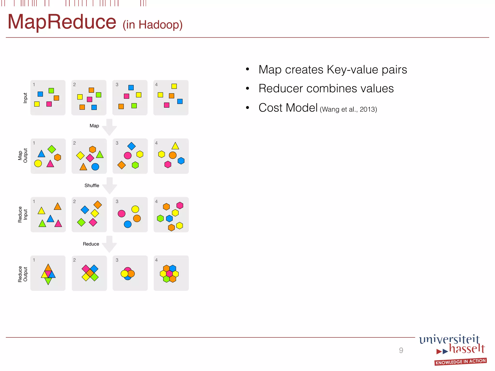
• Map creates Key-value pairs
• Reducer combines values
• Cost Model (Wang et al., 2013)
9
Map
Shuffle
Reduce
1 2 3 4
1 2 3 4
1 2 3 4
1 2 3 4
Input
Map
Output
Reduce
Input
Reduce
Output
Let I1 ∪ · · · ∪ Ik denote the partition of the input tuples
such that the mapper behaves uniformly1
on every data item
in Ii. Let Ni be the size (in MB) of Ii, and let Mi be the
size (in MB) of the intermediate data output by the mapper
on Ii. The cost of the map phase on Ii is:
costmap(Ni, Mi) = hrNi + mergemap(Mi) + lwMi,
where mergemap(Mi), denoting the cost of sort and merge in
the map stage, is expressed by
mergemap(Mi) = (lr + lw)Mi logD
(Mi+Mi)/mi
buf map
.
See Table 1 for the meaning of the variables hr, lw, lr, lw,
D, Mi, mi, and buf map.2
The total cost incurred in the map
phase equals the sum
k
i=1
costmap(Ni, Mi). (2)
Note that the cost model in [27, 36] defines the total cost
incurred in the map phase as
costmap
k
i=1
Ni,
k
i=1
Mi . (3)
The latter is not always accurate. Indeed, consider for in-
stance an MR job whose input consists of two relations R
and S where the map function outputs many key-value pairs
for each tuple in R and at most one key-value pair for each
tuple in S, e.g., because of filtering. This difference in map
output may lead to a non-proportional contribution of both
input relations to the total cost. Hence, as shown by Equa-
tion (2), we opt to consider different inputs separately. This
cannot be captured by map cost calculation of Equation (3),
as it considers the global average map output size in the cal-
culation of the merge cost. In Section 5, we illustrate this
problem by means of an experiment that confirms the effec-
tiveness of the proposed adjustment.
To analyze the cost in the reduce phase, let M = k
i=1 Mi.
The reduce stage involves (i) transferring the intermediate
data (i.e., the output of the map function) to the correct
reducer, (ii) merging the key-value pairs locally for each re-
ducer, (iii) applying the reduce function, and (iv) writing
the output to hdfs. Its cost will be
costred(M, K) = tM + mergered(M) + hwK,
where K is the size of the output of the reduce function (in
MB). The cost of merging equals
mergered(M) = (lr + lw)M logD
M/r
buf red
.
The total cost of an MR job equals the sum
costh +
k
costmap(Ni, Mi) + costred(M, K),
i=1 i=1
The latter is not always accurate. Indeed, consider for in-
stance an MR job whose input consists of two relations R
and S where the map function outputs many key-value pairs
for each tuple in R and at most one key-value pair for each
tuple in S, e.g., because of filtering. This difference in map
output may lead to a non-proportional contribution of both
input relations to the total cost. Hence, as shown by Equa-
tion (2), we opt to consider different inputs separately. This
cannot be captured by map cost calculation of Equation (3),
as it considers the global average map output size in the cal-
culation of the merge cost. In Section 5, we illustrate this
problem by means of an experiment that confirms the effec-
tiveness of the proposed adjustment.
To analyze the cost in the reduce phase, let M = k
i=1 Mi.
The reduce stage involves (i) transferring the intermediate
data (i.e., the output of the map function) to the correct
reducer, (ii) merging the key-value pairs locally for each re-
ducer, (iii) applying the reduce function, and (iv) writing
the output to hdfs. Its cost will be
costred(M, K) = tM + mergered(M) + hwK,
where K is the size of the output of the reduce function (in
MB). The cost of merging equals
mergered(M) = (lr + lw)M logD
M/r
buf red
.
The total cost of an MR job equals the sum
costh +
k
i=1
costmap(Ni, Mi) + costred(M, K),
where costh is the overhead cost of starting an MR job.
1 2 3
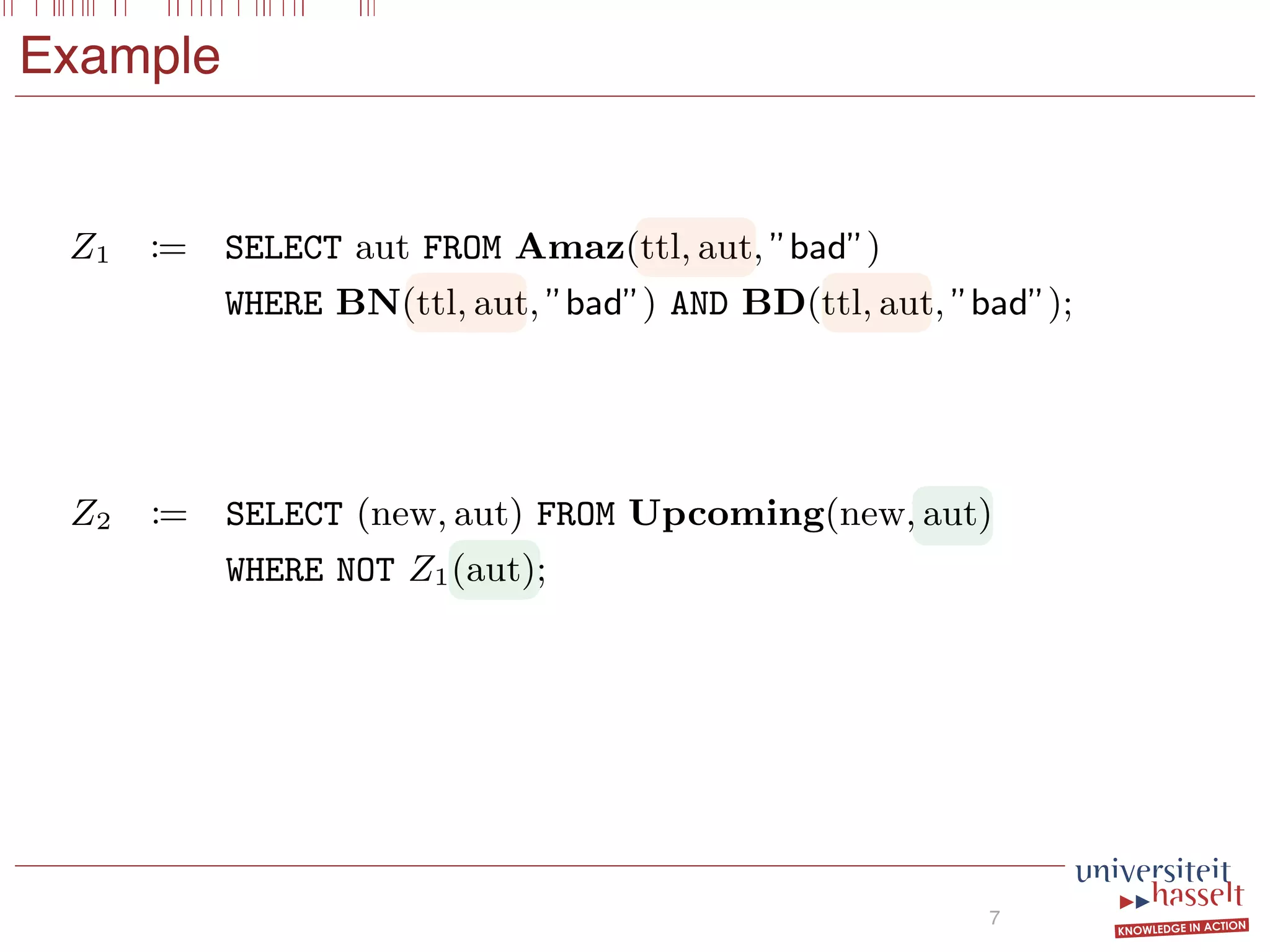
the atoms occurring in C are called the
We interpret Z as the output relation of
DB, the BSGF query (1) defines a new
ing all tuples ¯a for which there is a substi-
ariables occurring in ¯t such that σ(¯x) = ¯a,
d C evaluates to true in DB under substi-
he evaluation of C in DB under σ is de-
on the structure of C. If C is C1 OR C2,
T C1, the semantics is the usual boolean
C is an atom T(¯v) then C evaluates to
) T(¯v), i.e., if there exists a T-atom in
(σ(¯t)) on those positions where R(¯t) and
es.
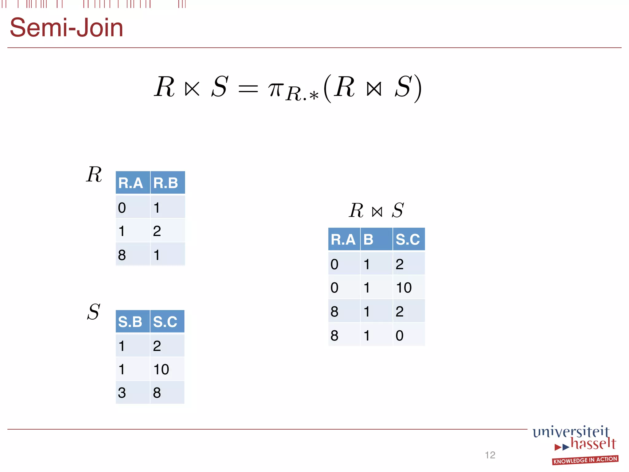
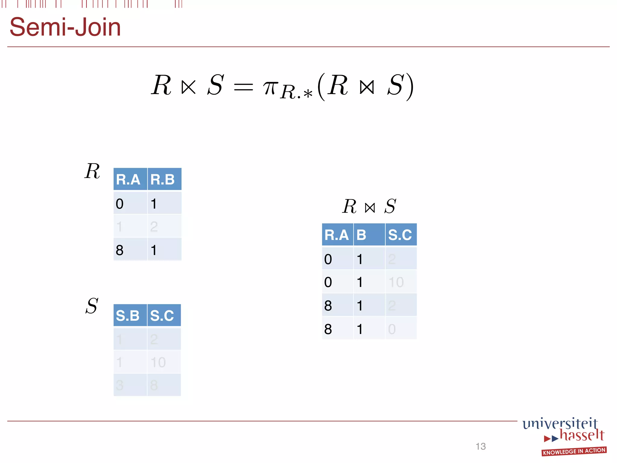
e intersection Z1 := R ∩ S and the dif-
− S between two relations R and S are
ws:
LECT ¯x FROM R(¯x) WHERE S(¯x);
LECT ¯x FROM R(¯x) WHERE NOT S(¯x);
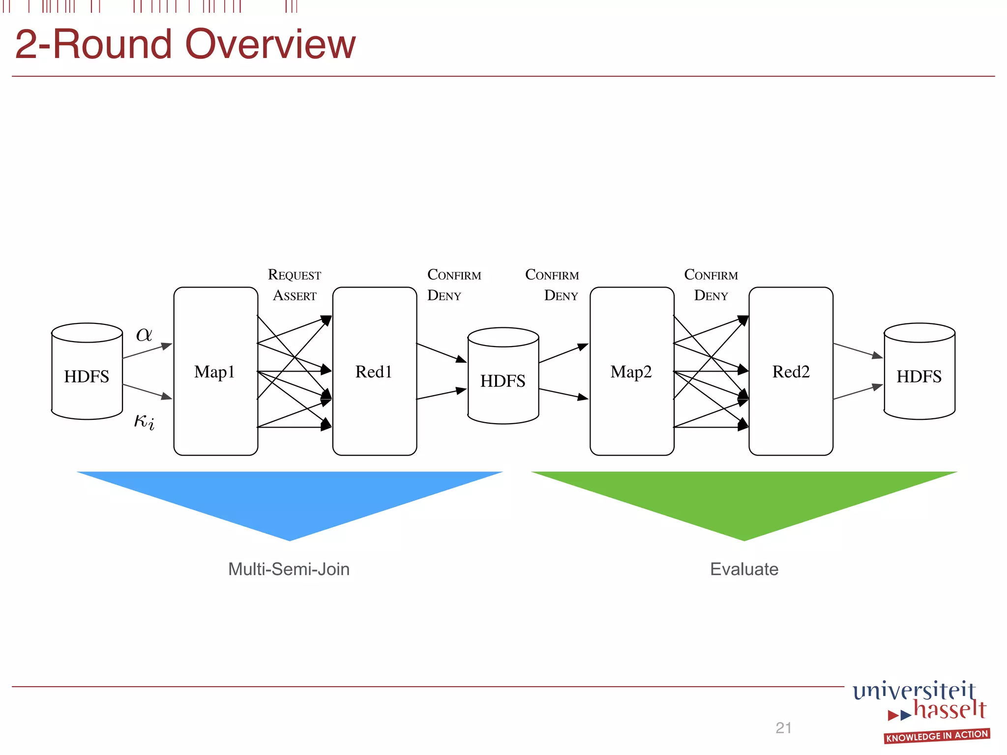
Input Intermediate Data Output
Map Phase
read → map → sort → merge →
Reduce Phase
trans. → merge → reduce → write
Figure 1: A depiction of the inner workings of Hadoop MR.
Remark 1. The syntax we use here differs from the tra-
ditional syntax of the Guarded Fragment [20], and is ac-
tually closer in spirit to join trees for acyclic conjunctive
queries [9, 11], although we do allow disjunction and nega-
tion in the where clause. In the traditional syntax, a pro-
jection in the guarded fragment is only allowed in the form
∃ ¯wR(¯x)∧ϕ(¯z) where all variables in ¯z must occur in ¯x. One
can obtain a query in the traditional syntax of the guarded
fragment from our syntax by adding extra projections for
the atoms in C. For example,
SELECT x FROM R(x, y) WHERE S(x, z1) AND NOT S(y, z2)
632 4 51
4
5
5
2](https://image.slidesharecdn.com/presentationvldb-160906170211/75/Parallel-Evaluation-of-Multi-Semi-Joins-12-2048.jpg)


![SELECT x,y FROM R(x,y)
WHERE [S(x,y) OR S(y,x)] AND T(x,z)
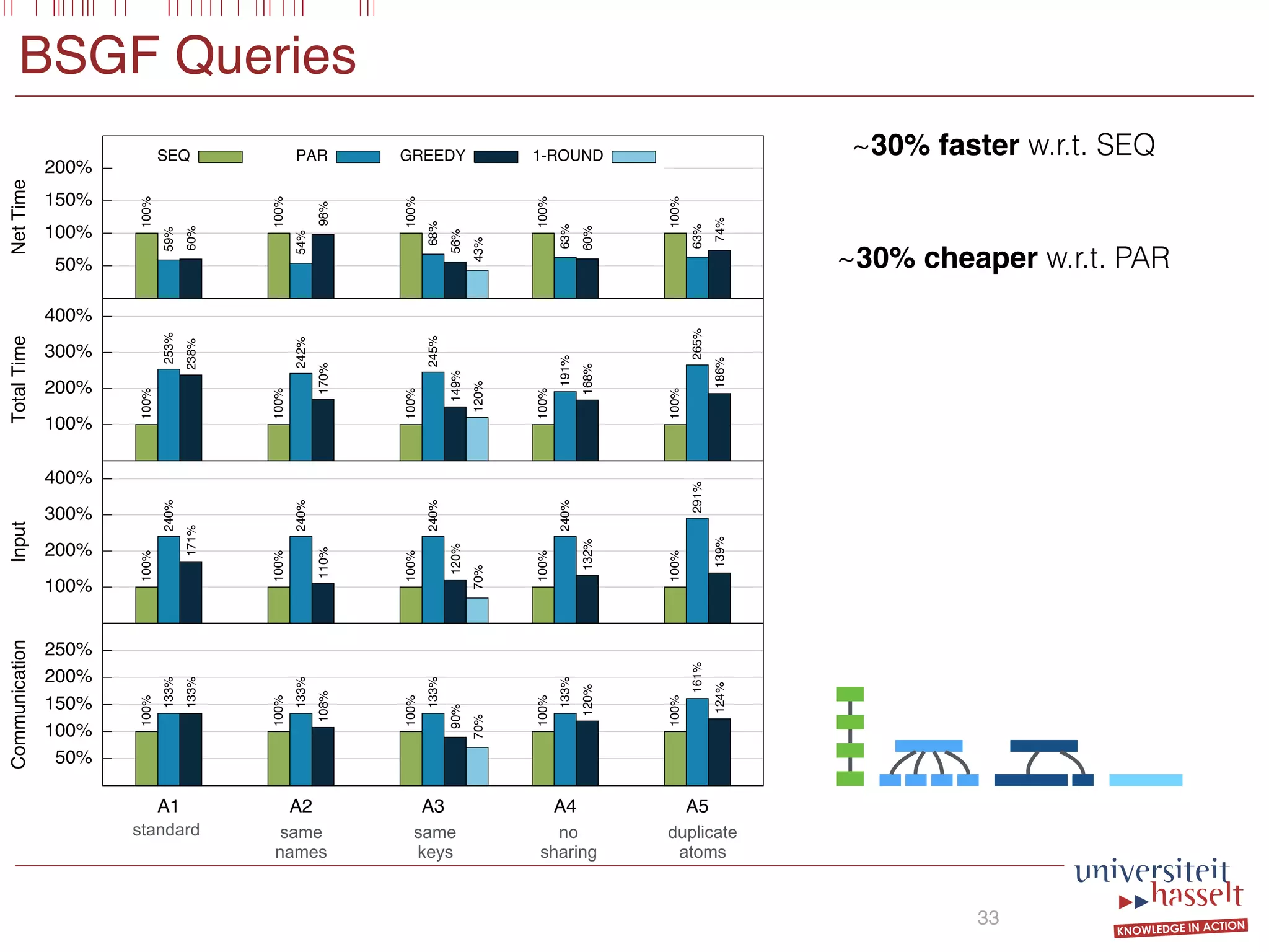
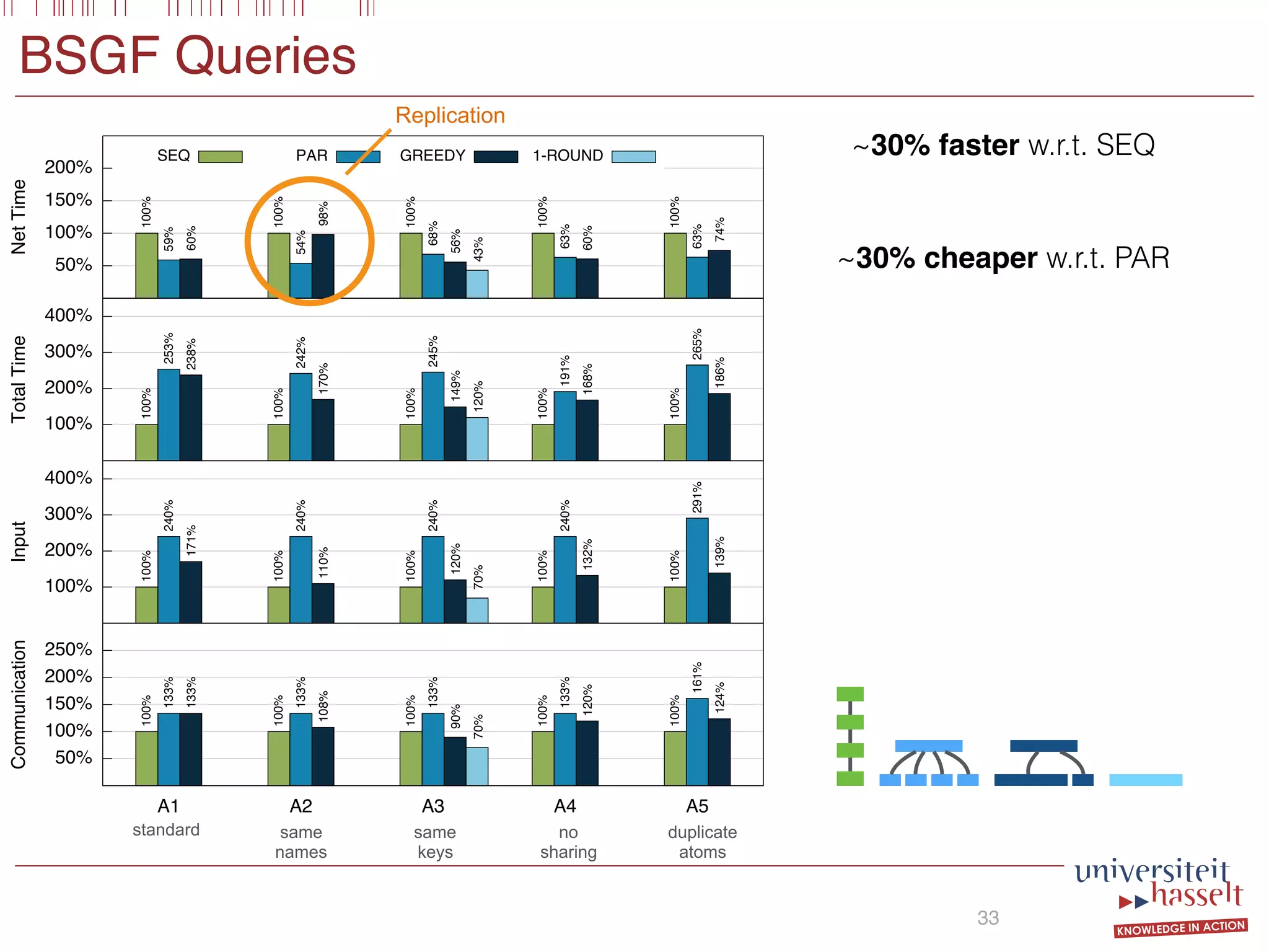
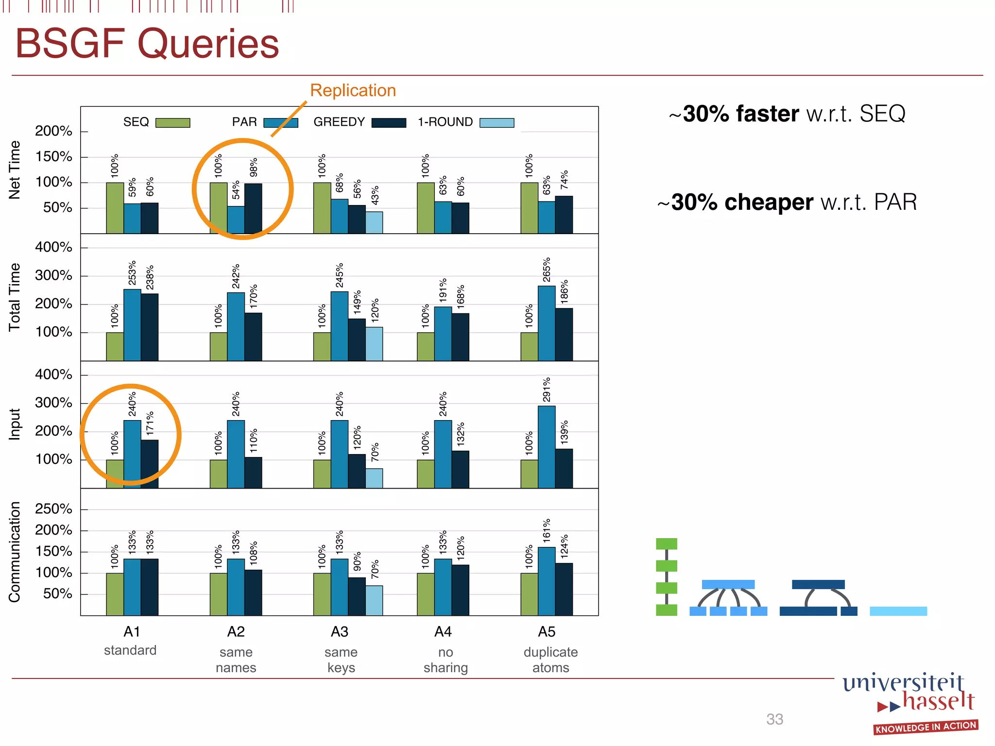
BSGF Queries
18
massively
g., [2–5, 7,
d in terms
me, amount
he number
m to bring
query end
important
no longer
ces such as
the cost is
Attribution-
view a copy
-nd/4.0/. For
n by emailing
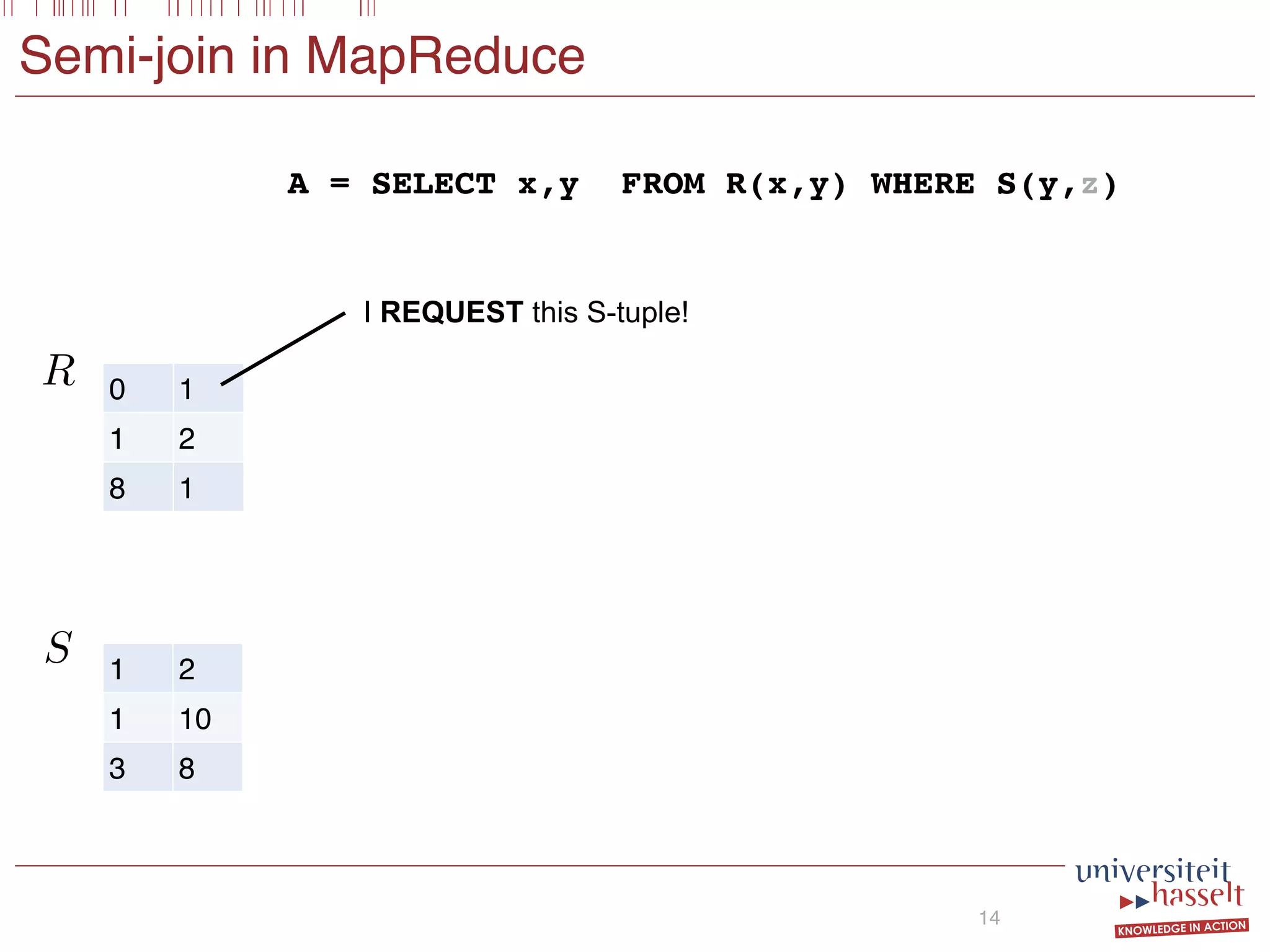
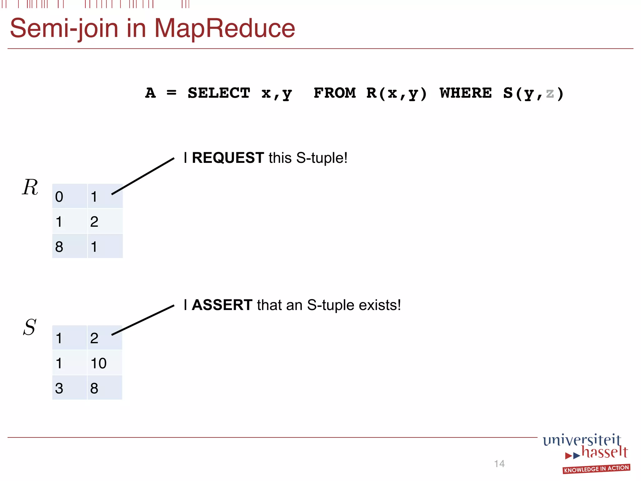
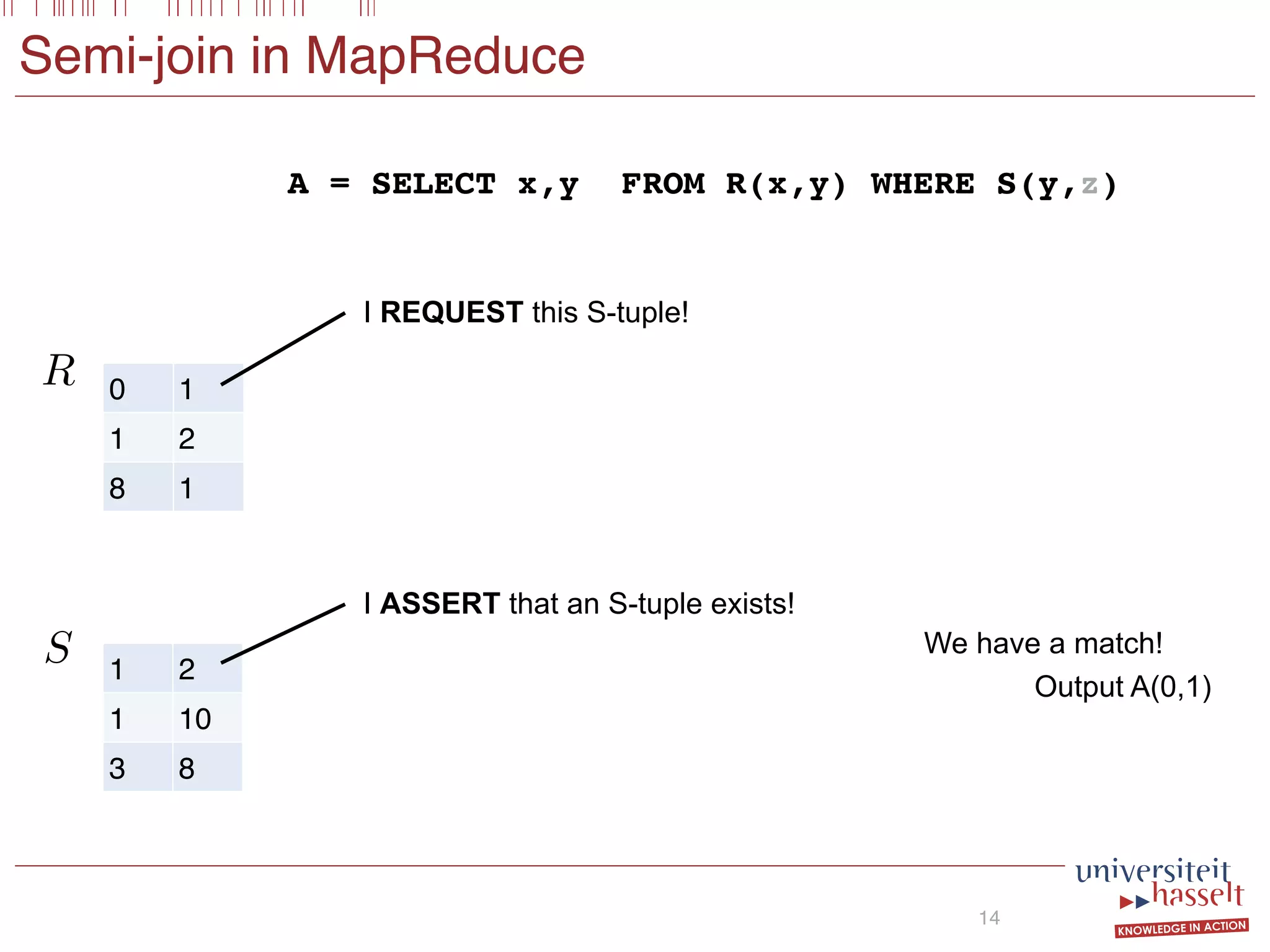
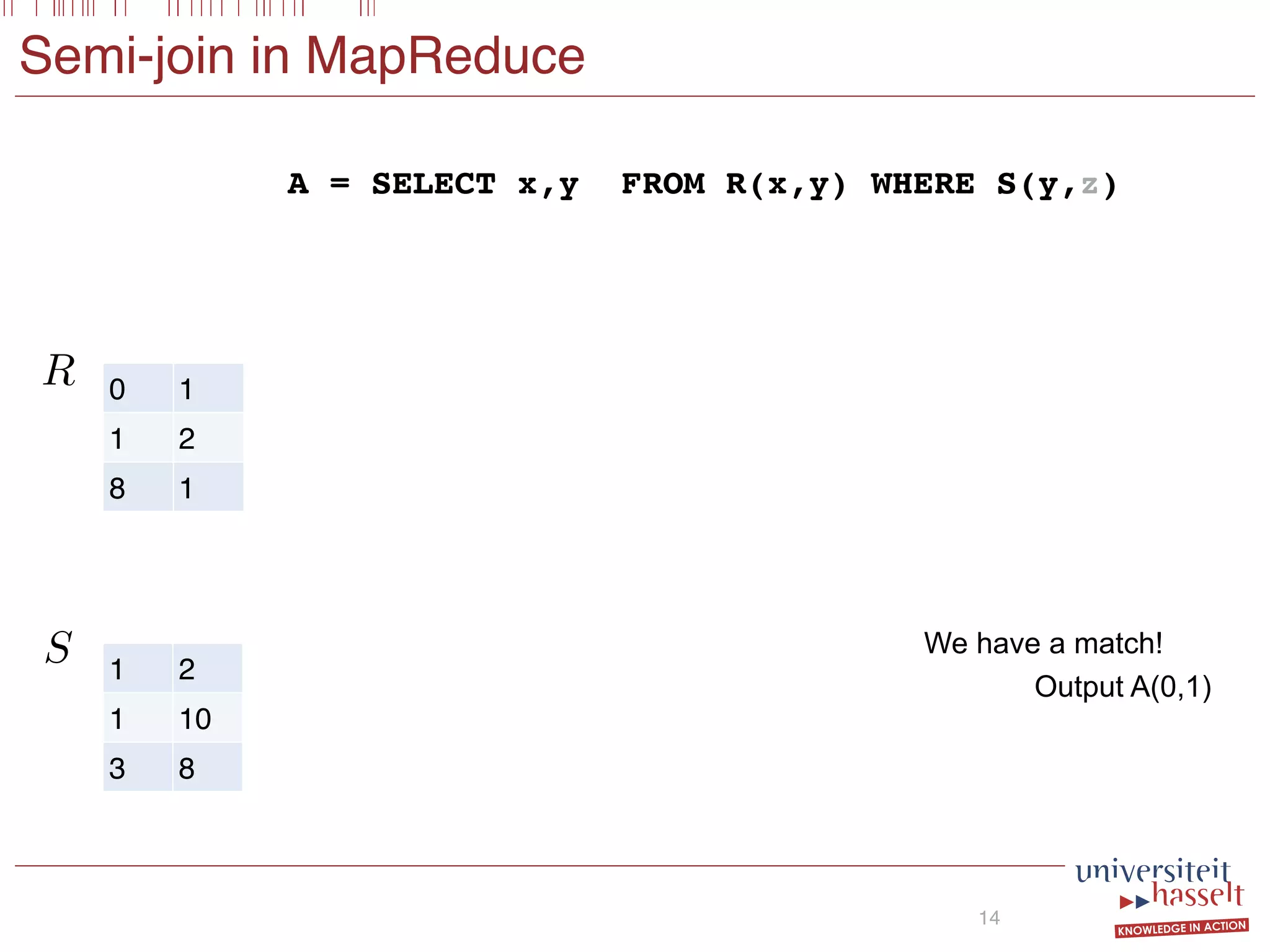
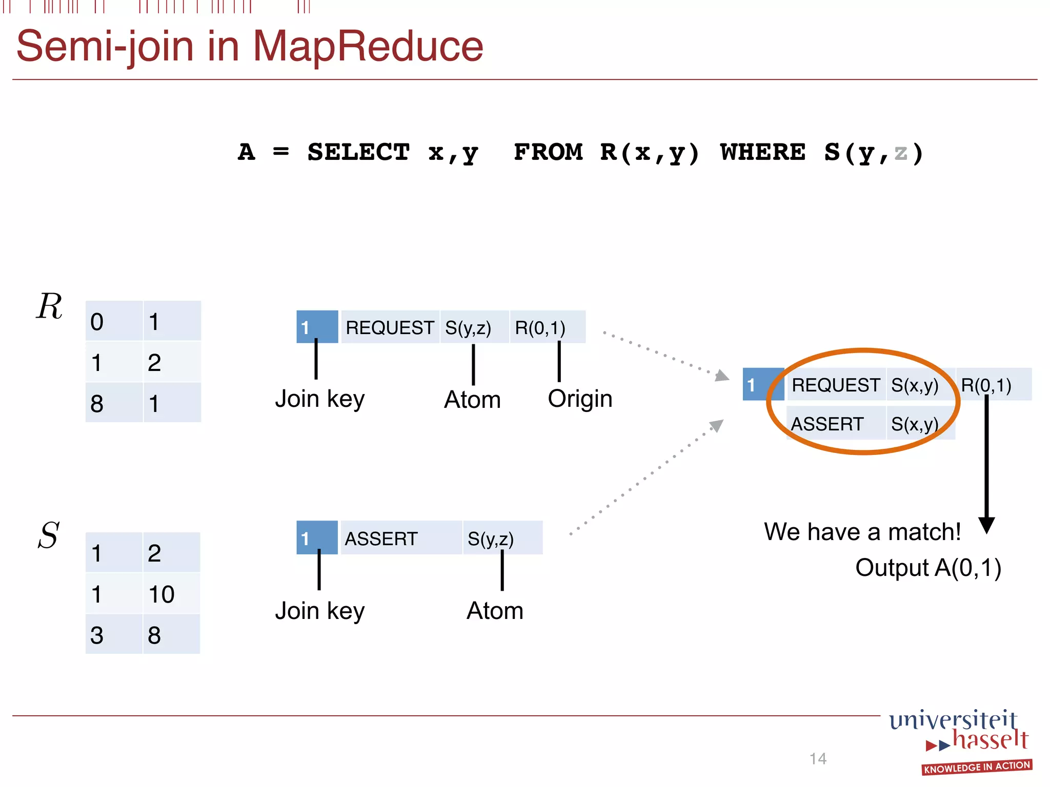
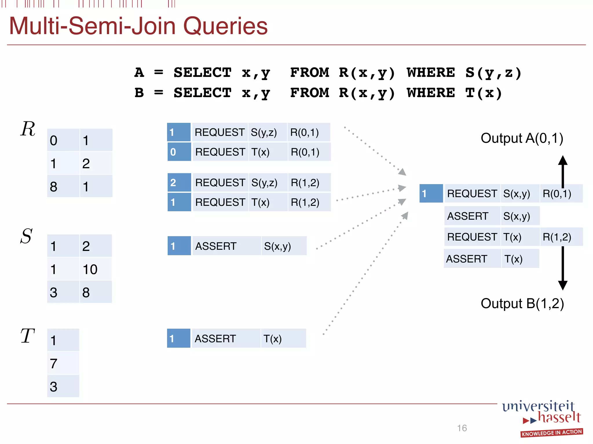
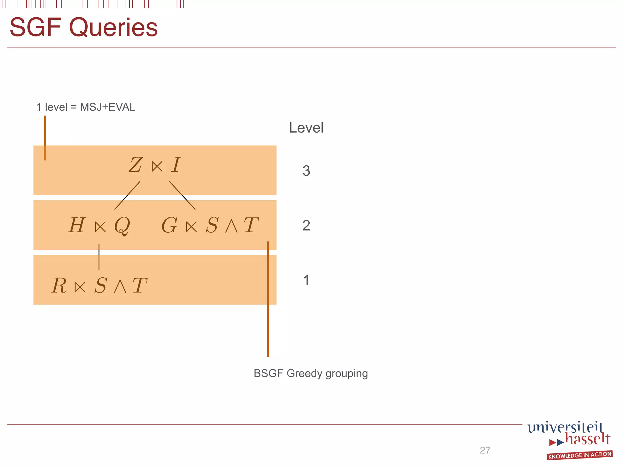
Consider the following SGF query Q:
SELECT (x, y) FROM R(x, y)
WHERE S(x, y) OR S(y, x) AND T(x, z)
Intuitively, this query asks for all pairs (x, y) in R for which
there exists some z such that (1) (x, y) or (y, x) occurs in
S and (2) (x, z) occurs in T. To evaluate Q it suffices to
compute the following semi-joins
X1 := R(x, y) S(x, y);
X2 := R(x, y) S(y, x);
X3 := R(x, y) T(x, z);
store the results in the binary relations X1, X2, or X3, and
subsequently compute ϕ := (X1 ∪X2)∩X3. Our multi-semi-
join operator MSJ(S) (defined in Section 4.2) takes a number
of semi-join-equations as input and exploits commonalities
between them to optimize evaluation. In our framework, a
possible query plan for query Q is of the form:
EVAL(R, ϕ)
MSJ(X1, X2) MSJ(X3)
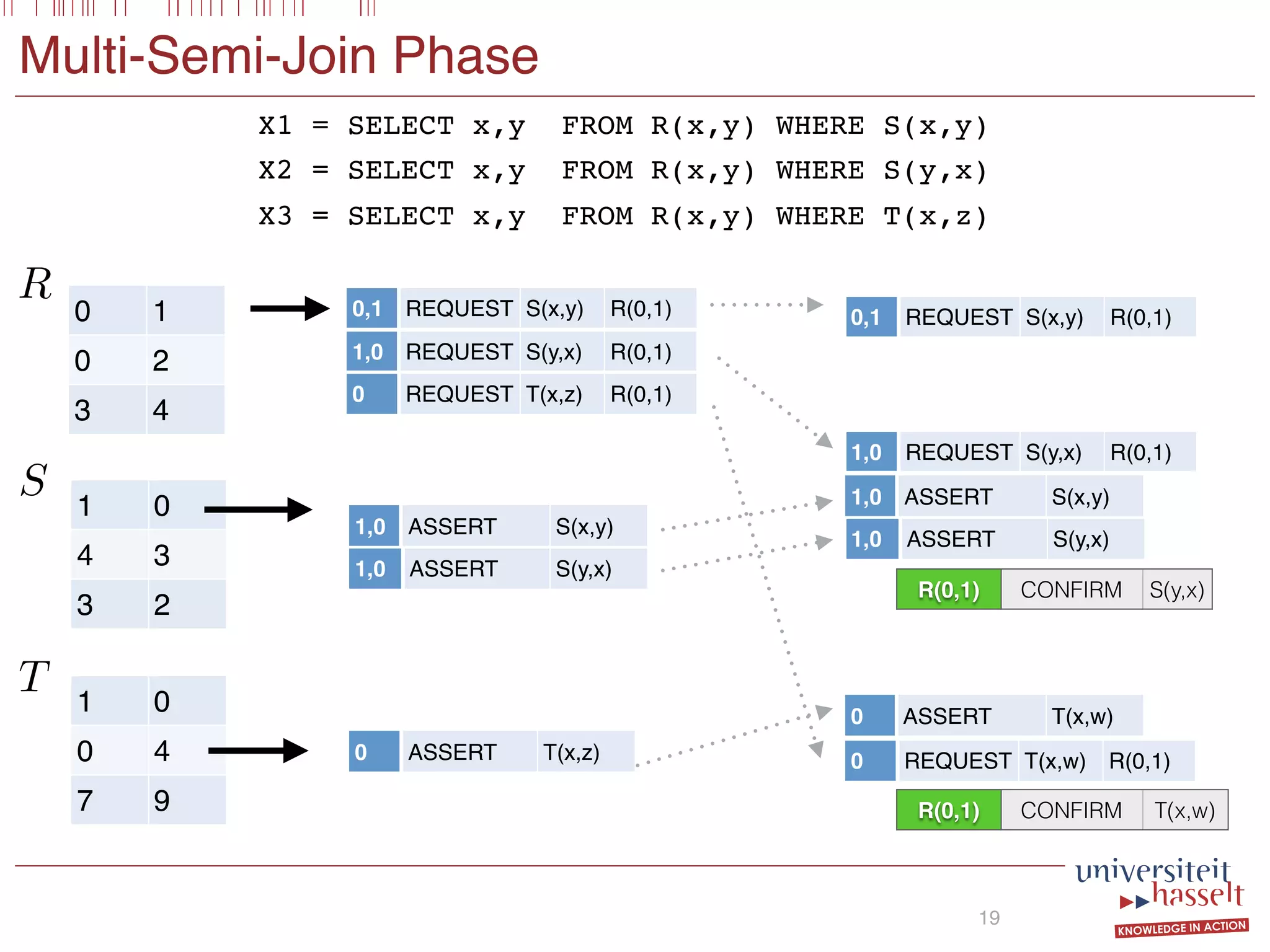
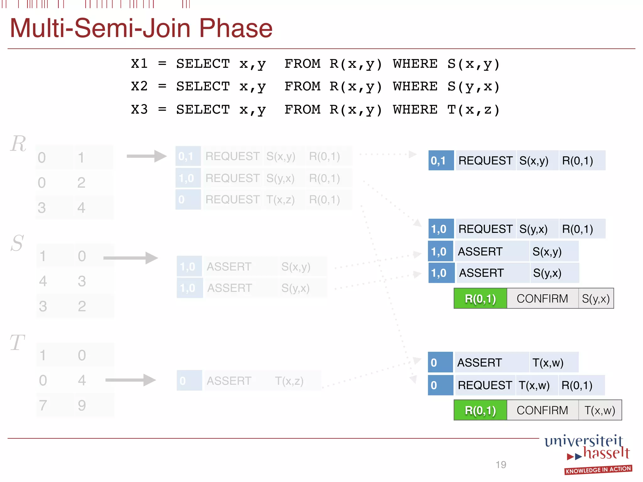
X1 = SELECT x,y FROM R(x,y) WHERE S(x,y)
X2 = SELECT x,y FROM R(x,y) WHERE S(y,x)
X3 = SELECT x,y FROM R(x,y) WHERE T(x,z)
SELECT x,y FROM R(x,y)
WHERE [X1(x,y) OR X2(x,y)] AND X3(x,y)
Semi-Joins
Boolean
Combination](https://image.slidesharecdn.com/presentationvldb-160906170211/75/Parallel-Evaluation-of-Multi-Semi-Joins-26-2048.jpg)
![EVAL Phase
20
R(0,1) CONFIRM S(y,x)
R(0,1) DENY S(x,y)
R(0,1) CONFIRM T(x,z)
R(3,4) CONFIRM S(y,x)
R(0,2) DENY S(y,x)
R(0,2) DENY S(x,y)
R(0,2) CONFIRM T(x,z)
R(3,4) DENY S(x,y)
R(3,4) DENY T(x,w)
R(0,1) CONFIRM S(y,x)
R(0,1) CONFIRM T(x,z)
R(3,4) CONFIRM S(y,x)
R(0,2) CONFIRM T(x,z)
(False _ True) ^ True ⌘ True
Z(0, 1)output
SELECT x,y FROM R(x,y)
WHERE [S(x,y) OR S(y,x)] AND T(x,z)
Implicit](https://image.slidesharecdn.com/presentationvldb-160906170211/75/Parallel-Evaluation-of-Multi-Semi-Joins-29-2048.jpg)
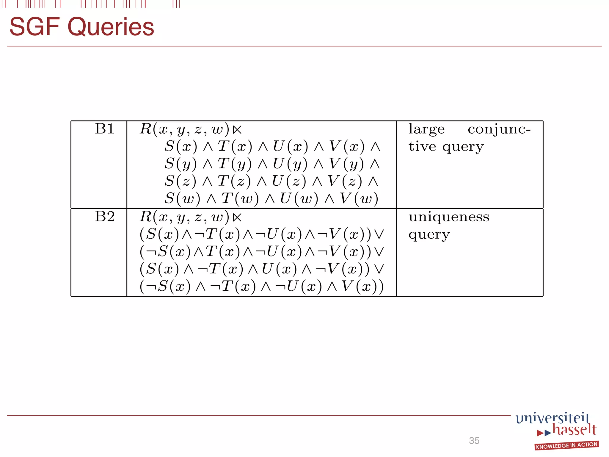
![Optimal Plan (BSGF)
23
136 Parallel Evaluation of Multi-Semi-Joins
EVAL
Z := X1 ^ (X2 _ ¬X3)
MSJ
X1 := R(x, y) n S(x, z)
MSJ
X2 := R(x, y) n T(y)
MSJ
X3 := R(x, y) n U(x)
(a)
EVAL
Z := X1 ^ (X2 _ ¬X3)
MSJ
X1 := R(x, y) n S(x, z)
X3 := R(x, y) n U(x)
MSJ
X2 := R(x, y) n T(y)
(b)
EVAL
Z := X1 ^ (X2 _ ¬X3)
MSJ
X1 := R(x, y) n S(x, z)
X2 := R(x, y) n T(y)
X3 := R(x, y) n U(x)
(c)
Figure 4.5: Some MapReduce query plan alternatives for the query given in
Example 4.13.
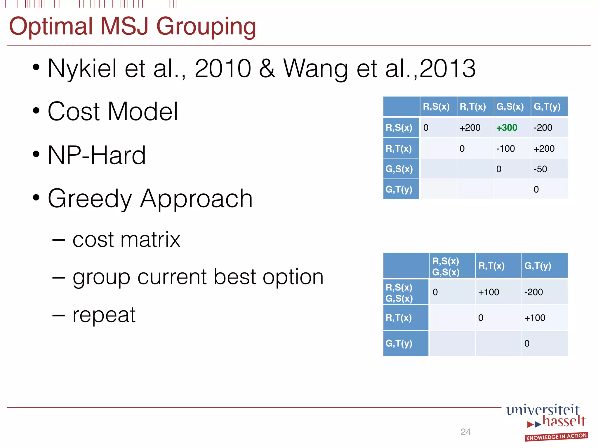
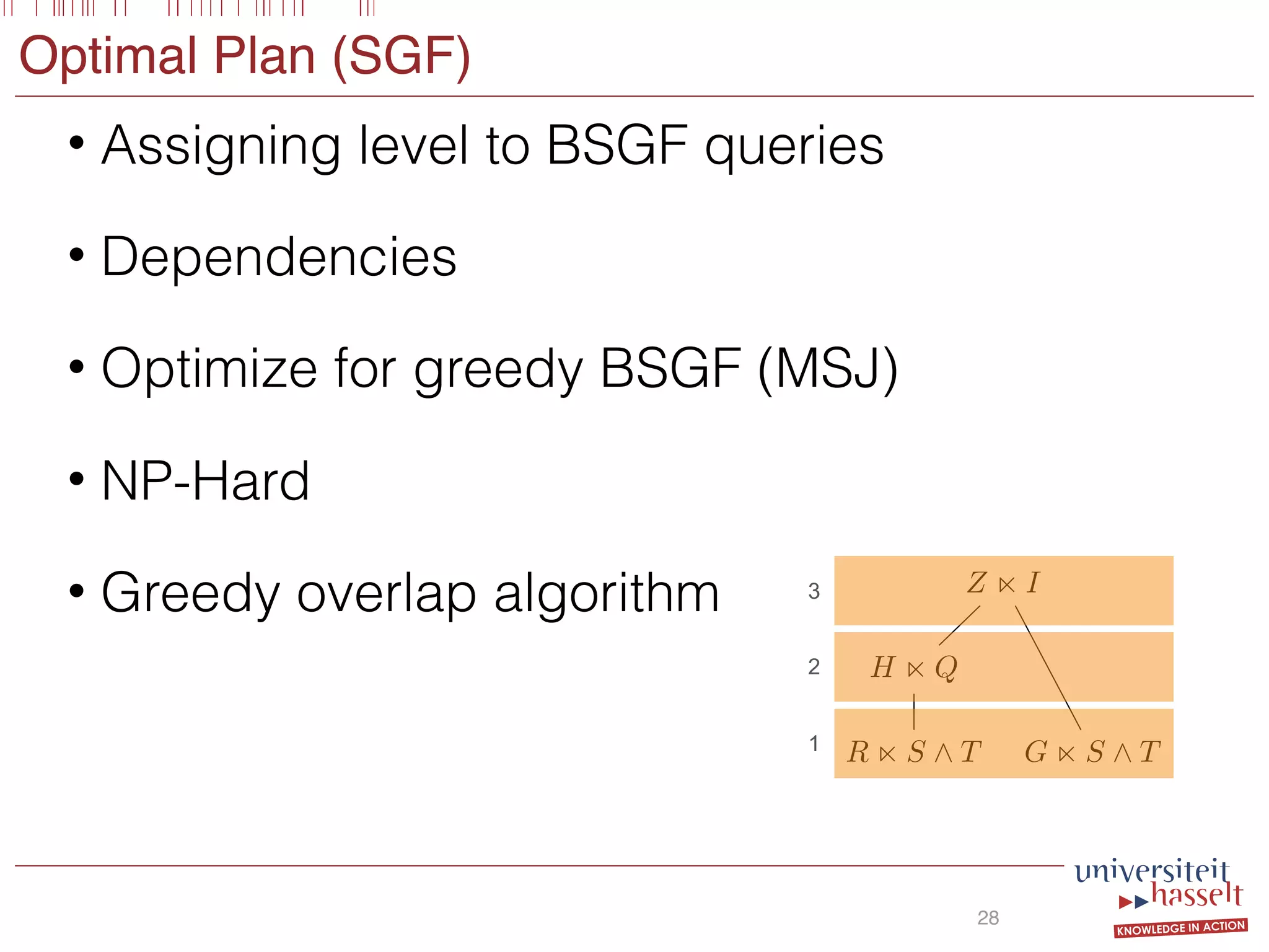
such that its total cost as computed in Equation (4.12) is minimal. The Scan-
Shared Optimal Grouping, which is known to be np-hard, is reducible to
this problem (see Nykiel et al. [139]). Stating it formally, we have:
Theorem 4.14. The decision variant of BSGF-Opt is np-complete.
136 Parallel Evaluation of Multi-Semi-Joins
EVAL
Z := X1 ^ (X2 _ ¬X3)
MSJ
X1 := R(x, y) n S(x, z)
MSJ
X2 := R(x, y) n T(y)
MSJ
X3 := R(x, y) n U(x)
(a)
EVAL
Z := X1 ^ (X2 _ ¬X3)
MSJ
X1 := R(x, y) n S(x, z)
X3 := R(x, y) n U(x)
MSJ
X2 := R(x, y) n T(y)
(b)
EVAL
Z := X1 ^ (X2 _ ¬X3)
MSJ
X1 := R(x, y) n S(x, z)
X2 := R(x, y) n T(y)
X3 := R(x, y) n U(x)
(c)
Figure 4.5: Some MapReduce query plan alternatives for the query given in
Example 4.13.
such that its total cost as computed in Equation (4.12) is minimal. The Scan-
136 Parallel Evaluation of Multi-Semi-Joins
EVAL
Z := X1 ^ (X2 _ ¬X3)
MSJ
X1 := R(x, y) n S(x, z)
MSJ
X2 := R(x, y) n T(y)
MSJ
X3 := R(x, y) n U(x)
(a)
EVAL
Z := X1 ^ (X2 _ ¬X3)
MSJ
X1 := R(x, y) n S(x, z)
X3 := R(x, y) n U(x)
MSJ
X2 := R(x, y) n T(y)
(b)
EVAL
Z := X1 ^ (X2 _ ¬X3)
MSJ
X1 := R(x, y) n S(x, z)
X2 := R(x, y) n T(y)
X3 := R(x, y) n U(x)
(c)
Figure 4.5: Some MapReduce query plan alternatives for the query given in
Example 4.13.
such that its total cost as computed in Equation (4.12) is minimal. The Scan-](https://image.slidesharecdn.com/presentationvldb-160906170211/75/Parallel-Evaluation-of-Multi-Semi-Joins-34-2048.jpg)
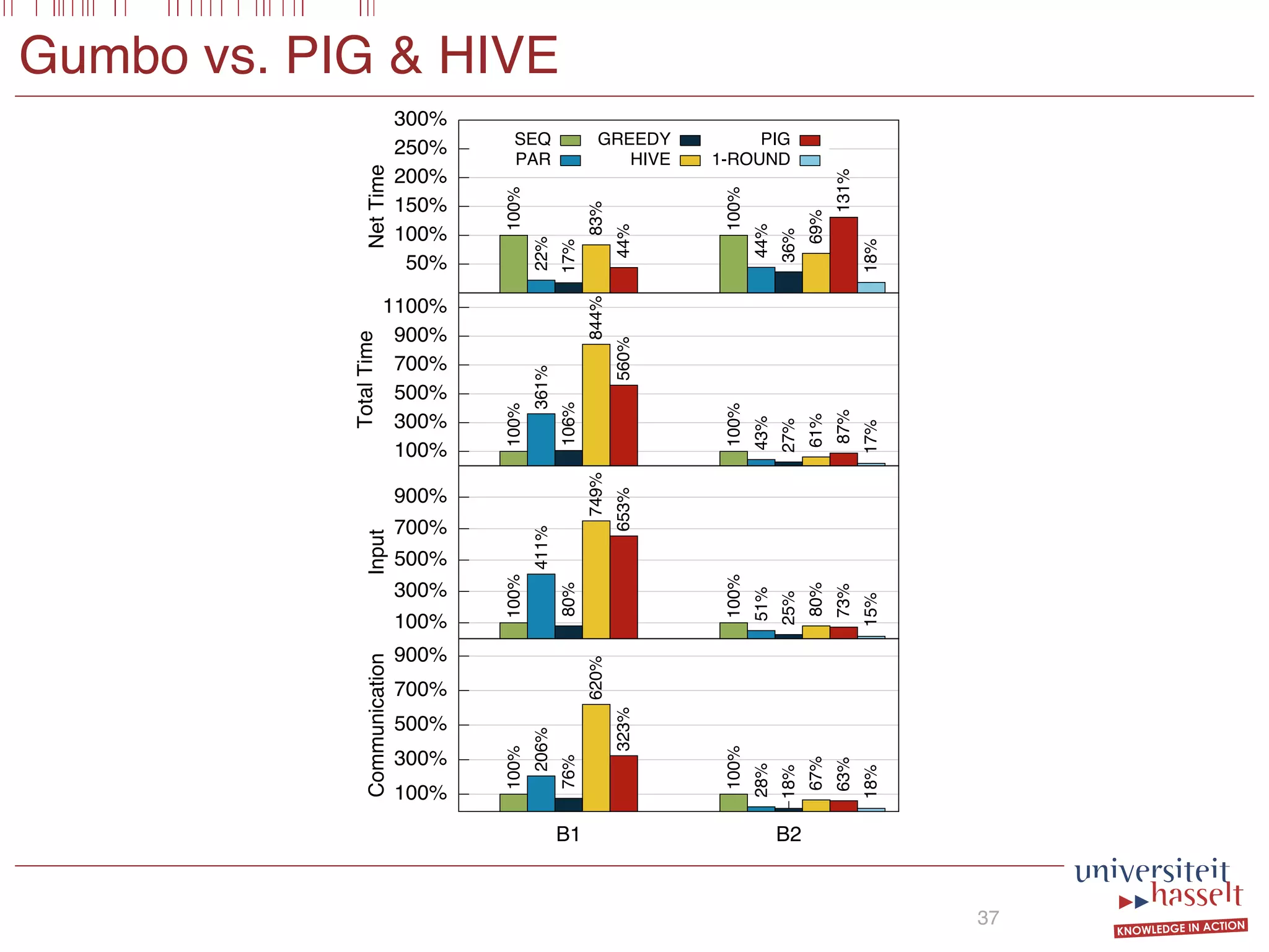


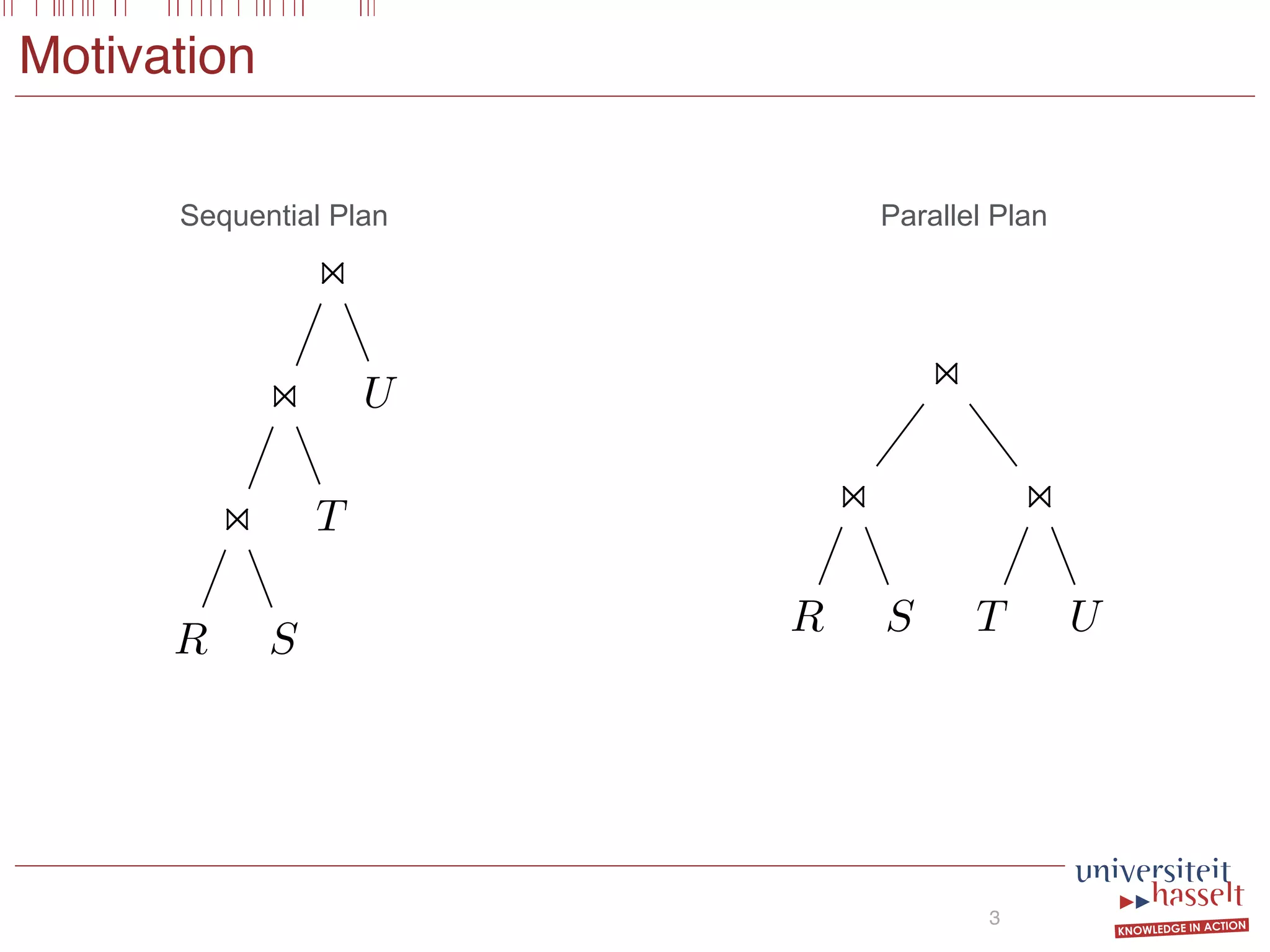
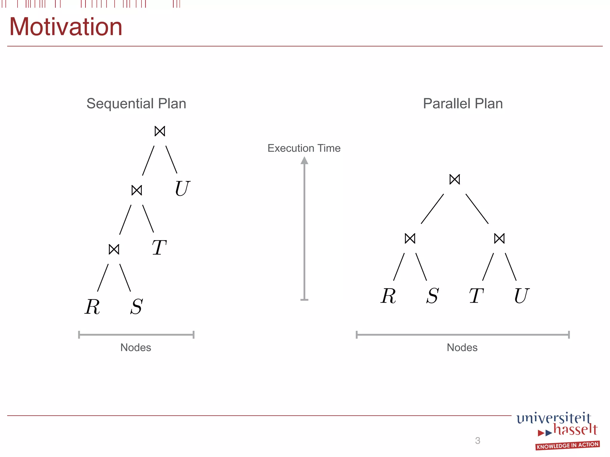
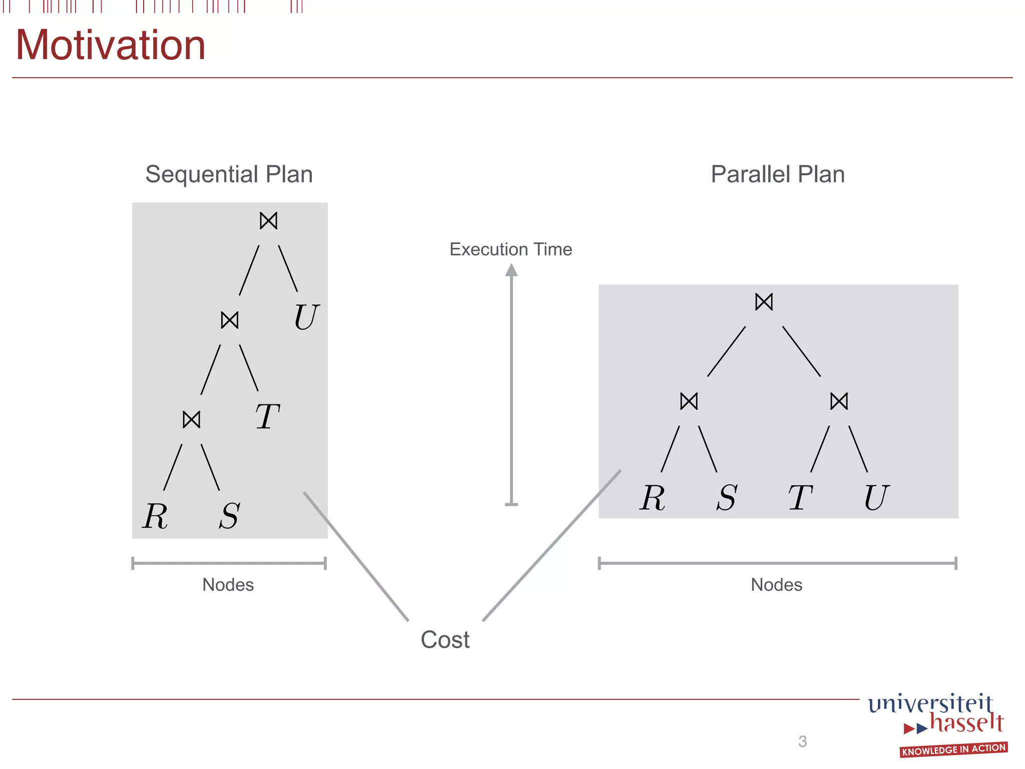
This document discusses the parallel evaluation of multi-semi-joins, highlighting techniques utilizing MapReduce to optimize query execution time and cost through a strictly guarded fragment (SGF) query language. It demonstrates the evaluation process for semi-joins, multi-semi-joins, and provides a cost model for the MapReduce framework. The document also emphasizes the importance of separating different inputs during the map phase to ensure accurate cost calculation and presents experimental results to validate the proposed adjustments.


![[DSC Europe 25] Dusan Nesic - Securing Tomorrow’s Infrastructure: Why Cyber-P...](https://cdn.slidesharecdn.com/ss_thumbnails/qikbszfftyowjm2q6duw-1-251211083848-8f2ead6b-thumbnail.jpg?width=640&height=640&fit=bounds)


![[DSC Europe 25] Uros Pesic - The Reality of AI in Marketing.pdf](https://cdn.slidesharecdn.com/ss_thumbnails/rtkodnmtycovsllvzsyn-9-251215095918-b0c6bfe3-thumbnail.jpg?width=640&height=640&fit=bounds)

![[DSC Europe 25] Jon Dajci - Bridging TradFi and DeFi: Building the Future of ...](https://cdn.slidesharecdn.com/ss_thumbnails/fqmhfvlbqhkihjvqvhmu-7-251211083849-6af7e325-thumbnail.jpg?width=640&height=640&fit=bounds)

![[DSC Europe 25] Nikolay Burlutskiy - Best Practices for Building Enterprise M...](https://cdn.slidesharecdn.com/ss_thumbnails/uirvaiuvq8y1w8hzd9tx-7-251212103249-2619edb4-thumbnail.jpg?width=640&height=640&fit=bounds)
![[DSC Europe 25] Dunja Adzic Jovanovic - AI and Cybersecurity: Defending Data ...](https://cdn.slidesharecdn.com/ss_thumbnails/o1zylpbhrtwnixxq2xj8-7-251211083048-185086f6-thumbnail.jpg?width=640&height=640&fit=bounds)
![[DSC Europe 25] Branko Urosevic -Rethinking Financial Talent: Integrating Cod...](https://cdn.slidesharecdn.com/ss_thumbnails/8jjrus8ttko6qj64f58f-3-251212103250-642c6374-thumbnail.jpg?width=640&height=640&fit=bounds)
![[DSC Europe 25] Jovan Bogicevic - Legacy to AI-Driven Defense: Transforming D...](https://cdn.slidesharecdn.com/ss_thumbnails/rsarluadt563hntyfc8q-3-251211083849-3e7bc4c0-thumbnail.jpg?width=640&height=640&fit=bounds)
