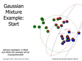
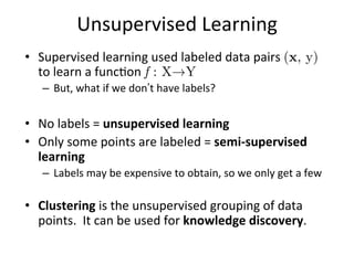
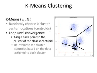
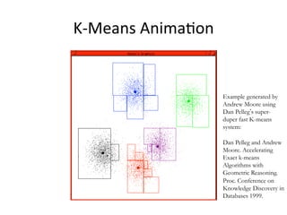
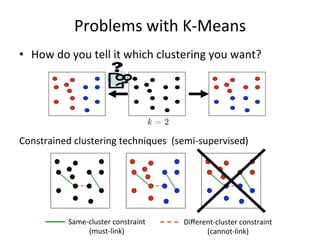
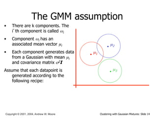
This document discusses unsupervised learning techniques for clustering data, specifically K-Means clustering and Gaussian Mixture Models. It explains that K-Means clustering groups data by assigning each point to the nearest cluster center and iteratively updating the cluster centers. Gaussian Mixture Models assume the data is generated from a mixture of Gaussian distributions and uses the Expectation-Maximization algorithm to estimate the parameters of the mixture components.


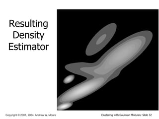
![Clustering with Gaussian Mixtures: Slide 20
Copyright © 2001, 2004, Andrew W. Moore
E.M. for General GMMs
Iterate. On the t’th iteration let our estimates be
λt = { µ1(t), µ2(t) … µc(t), Σ1(t), Σ2(t) … Σc(t), p1(t), p2(t) … pc(t) }
E-step: Compute “expected” clusters of all datapoints
( ) ( ) ( )
( )
( )
( )
∑
=
Σ
Σ
=
= c
j
j
j
j
j
k
i
i
i
i
k
t
k
t
i
t
i
k
t
k
i
t
p
t
t
w
x
t
p
t
t
w
x
x
w
w
x
x
w
1
)
(
)
(
),
(
,
p
)
(
)
(
),
(
,
p
p
P
,
p
,
P
µ
µ
λ
λ
λ
λ
M-step: Estimate µ, Σ given our data’s class membership distributions
pi(t) is shorthand
for estimate of
P(ωi) on t’th
iteration
( )
( )
( )
∑
∑
=
+
k
t
k
i
k
k
t
k
i
i
x
w
x
x
w
t
λ
λ
,
P
,
P
1
µ ( )
( ) ( )
[ ] ( )
[ ]
( )
∑
∑ +
−
+
−
=
+
Σ
k
t
k
i
T
i
k
i
k
k
t
k
i
i
x
w
t
x
t
x
x
w
t
λ
µ
µ
λ
,
P
1
1
,
P
1
( )
( )
R
x
w
t
p k
t
k
i
i
∑
=
+
λ
,
P
1 R = #records
Just evaluate a
Gaussian at xk](https://image.slidesharecdn.com/13unsupervisedlearning-231023094004-cfb60bf2/85/13_Unsupervised-Learning-pdf-20-320.jpg)