Download to read offline
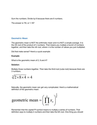

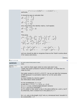
![set. For example, the geometric mean of 5, 7, 2, 1 is (5 × 7 × 2 × 1)1/4
= 2.893.
Alternatively, if you log transform each of the individual units the geometric will be the
exponential of the arithmetic mean of these log-transformed values. So, reusing the
example above, exp [ ( ln(5) + ln(7) + ln(2) + ln(1) ) / 4 ] = 2.893.
Geometric Mean
Arithmetic Mean
An arithmetic average is the sum of a series of numbers divided by the count of that
series of numbers.
If you were asked to find the class (arithmetic) average of test scores, you would simply
add up all the test scores of the students, and then divide that sum by the number of
students. For example, if five students took an exam and their scores were 60%, 70%,
80%, 90% and 100%, the arithmetic class average would be 80%.
This would be calculated as: (0.6 + 0.7 + 0.8 + 0.9 + 1.0) / 5 = 0.8.
The reason you use an arithmetic average for test scores is that each test score is an
independent event. If one student happens to perform poorly on the exam, the next
student's chances of doing poor (or well) on the exam isn't affected. In other words,
each student's score is independent of the all other students' scores. However, there
are some instances, particularly in the world of finance, where an arithmetic mean is not
an appropriate method for calculating an average.
Consider your investment returns, for example. Suppose you have invested your
savings in the stock market for five years. If your returns each year were 90%, 10%,
20%, 30% and -90%, what would your average return be during this period? Well,
taking the simple arithmetic average, you would get an answer of 12%. Not too shabby,
you might think.
However, when it comes to annual investment returns, the numbers are not](https://image.slidesharecdn.com/1561-maths-161031144107/85/1561-maths-4-320.jpg)
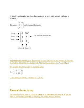
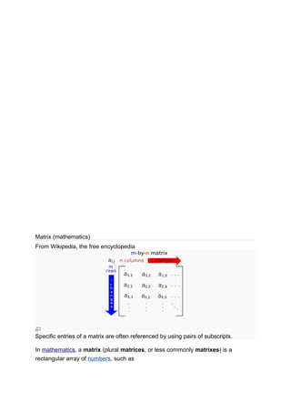
![independent of each other. If you lose a ton of money one year, you have that much
less capital to generate returns during the following years, and vice versa. Because of
this reality, we need to calculate the geometric average of your investment returns in
order to get an accurate measurement of what your actual average annual return over
the five-year period is.
To do this, we simply add one to each number (to avoid any problems with negative
percentages). Then, multiply all the numbers together, and raise their product to the
power of one divided by the count of the numbers in the series. And you're finished -
just don't forget to subtract one from the result!
That's quite a mouthful, but on paper it's actually not that complex. Returning to our
example, let's calculate the geometric average: Our returns were 90%, 10%, 20%, 30%
and -90%, so we plug them into the formula as [(1.9 x 1.1 x 1.2 x 1.3 x 0.1) ^ 1/5] - 1.
This equals a geometric average annual return of -20.08%. That's a heck of a lot worse
than the 12% arithmetic average we calculated earlier, and unfortunately it's also the
number that represents reality in this case.
It may seem confusing as to why geometric average returns are more accurate than
arithmetic average returns, but look at it this way: if you lose 100% of your capital in one
year, you don't have any hope of making a return on it during the next year. In other
words, investment returns are not independent of each other, so they require a
geometric average to represent their mean.](https://image.slidesharecdn.com/1561-maths-161031144107/85/1561-maths-5-320.jpg)
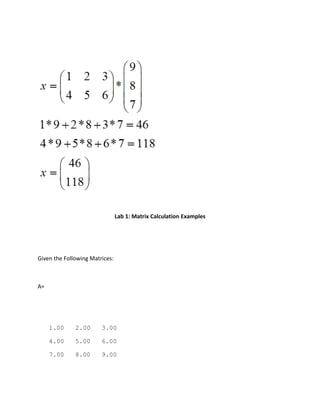
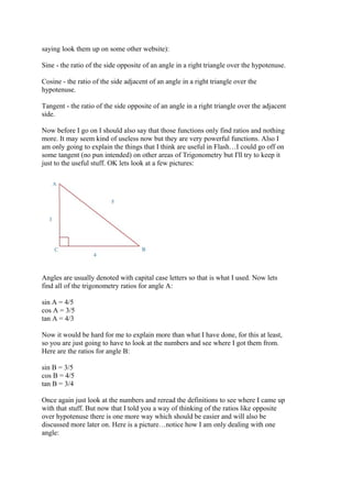
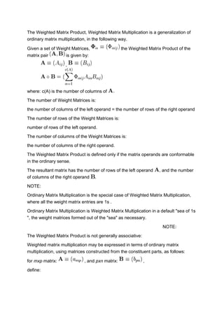
![Each element is defined by its position in the matrix.
In a matrix A, an element in row i and column j is represented by aij
Example:
a11 (read as ‘a one one ’)= 2 (first row, first column)
a12 (read as ‘a one two') = 4 (first row, second column)
a13 = 5, a21 = 7, a22 = 8, a23 = 9
Matrix Multiplication
There are two matrix operations
which we will use in our matrix transformations, multiplying (concatenating) two matrices,
and transforming a vector by a matrix. We will now examine the first of these two
operations, matrix multiplication.
Matrix multiplication is the operation by which one matrix is transformed by another. A very
important thing to remember is that matrix multiplication is not commutative. That is, [a] *
[b] != [b] * [a]. For now, it will suffice to say that a matrix multiplication stores the results
of the sum of the products of matrix rows and columns. Here is some example code of a
matrix multiplication routine which multiplies matrix [a] * matrix [b], then copies the result
to matrix a.
void matmult(float a[4][4], float b[4][4])](https://image.slidesharecdn.com/1561-maths-161031144107/85/1561-maths-7-320.jpg)
![{
float temp[4][4]; // temporary matrix for storing result
int i, j; // row and column counters
for (j = 0; j < 4; j++) // transform by columns first
for (i = 0; i < 4; i++) // then by rows
temp[i][j] = a[i][0] * b[0][j] + a[i][1] * b[1][j] +
a[i][2] * b[2][j] + a[i][3] * b[3][j];
for (i = 0; i < 4; i++) // copy result matrix into matrix a
for (j = 0; j < 4; j++)
a[i][j] = temp[i][j];
}
I have been informed that there is a faster way of multiplying matrices, which involves
taking the dot product of rows and columns. However, I have yet to implement such a
method, so I will not discuss it here at this time.
Transforming a Vector by a Matrix
This is the second operation
which is required for our matrix transformations. It involves projecting a stationary vector
onto transformed axis vectors using the dot product. One dot product is performed for each
coordinate axis.
x = x0 * matrix[0][0] + y0 * matrix[1][0] + z0 * matrix[2][0] +
w0 * matrix[3][0];
y = x0 * matrix[0][1] + y0 * matrix[1][1] + z0 * matrix[2][1] +
w0 * matrix[3][1];
z = x0 * matrix[0][2] + y0 * matrix[1][2] + z0 * matrix[2][2] +
w0 * matrix[3][2];
The x0, y0, etc. coordinates are the original object space coordinates for the vector. That is,
they never change due to transformation.
"Alright," you say. "Where did all the w coordinates come from???" Good question :) The w
coordinates come from what is known as a homogenous coordinate system, which is
basically a way to represent 3d space in terms of a 4d matrix. Because we are limiting
ourselves to 3d, we pick a constant, nonzero value for w (1.0 is a good choice, since
anything * 1.0 = itself). If we use this identity axiom, we can eliminate a multiply from each
of the dot products:
x = x0 * matrix[0][0] + y0 * matrix[1][0] + z0 * matrix[2][0] +
matrix[3][0];
y = x0 * matrix[0][1] + y0 * matrix[1][1] + z0 * matrix[2][1] +
matrix[3][1];](https://image.slidesharecdn.com/1561-maths-161031144107/85/1561-maths-8-320.jpg)
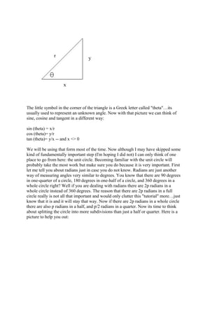
![z = x0 * matrix[0][2] + y0 * matrix[1][2] + z0 * matrix[2][2] +
matrix[3][2];
These are the formulas you should use to transform a vector by a matrix.
Object Space Transformations
Now that we know how to multiply matrices together, we can implement the actual formulas
used in our transformations. There are three operations performed on a vector by a matrix
transformation: translation, rotation, and scaling.
Translation can best be described as linear change in position. This change can be
represented by a delta vector [dx, dy, dz], where dx represents the change in the object's x
position, dy represents the change in its y position, and dz its z position.
If done correctly, object space translation allows objects to translate forward/backward,
left/right, and up/down, relative to the current orientation of the object. Using our airplane
as an example, if the nose of the airplane is oriented along the object's local z axis, then
translating the airplane in the +z direction will make the airplane move forward (the
direction in which its nose is pointing) regardless of the airplane's orientation.
Here is the translation matrix:
+= =+
| += =+ += =+ += =+ += += |
| | | | | | | | | |
| | 1 | | 0 | | 0 | | 0 | |
| | | | | | | | | |
| | | | | | | | | |
| | 0 | | 1 | | 0 | | 0 | |
| | | | | | | | | |
| | | | | | | | | |
| | 0 | | 0 | | 1 | | 0 | |
| += =+ += =+ += =+ | | |
| +===============+ | | |
| dy dx dz | 1 | |
| +===============+ += =+ |
+= =+
where [dx, dy, dz] is the displacement vector. After this operation, the object will have
moved in its own coordinate system, according to the displacement (translation) vector.
The next operation that is performed by our matrix transformation is rotation. Rotation can
be described as circular motion about some axis, in this case the axis is one of the object's
local axes. Since there are three axes in each object, we need to rotate around each of
them. Here are the matrices for rotation about each axis:
about the x axis:](https://image.slidesharecdn.com/1561-maths-161031144107/85/1561-maths-9-320.jpg)

![The cx, sx, cy, sy, cz, and sz variables are the values of the cosines and sines of the angles
of rotation about the x, y, and z axes, respectively. Remeber that the angles used represent
angular displacement just as the values used in the translation step denote a linear
displacement. Correct transformation CANNOT be accomplished with matrix multiplication if
you use the cumulative angles of rotation. I have been told that quaternions are able to
perform this operation correctly, however I know nothing of quaternions and how they are
implemented. The incremental angles used here represent rotation from the current object
orientation. In other words, by rotating 1 degree about the z axis, you are telling your
object "Rotate 1 degree about your z axis, regardless of your current orientation, and
regardless of how you got to that orientation." If you think about it a bit, you will realize
that this is how the real world operates. In object space, the series of rotations an object
undergoes to attain a certain orientation have no effect on the object space results of any
upcoming rotations.
Now that we know the matrix formulas for translation and rotation, we can combine them to
transform our objects. The formula for transformations in object space is
[O] = [O] * [T] * [X] * [Y] * [Z]
where O is the object's matrix, T is the translation matrix, and X, Y, and Z are the rotation
matrices for their respective axes. Remember, that order of matrix multiplication is very
important!
The recursive assignment of O poses a question: What is the original value of the object
matrix? To eliminate any terrible errors in transformation, the matrices which store an
object's orientation should always be initialized to identity.
Matrix Multiplication
You probably know what a matrix is already if you are interested in matrix multiplication.
However, a quick example won't hurt. A matrix is just a two-dimensional group of
numbers. Instead of a list, called a vector, a matrix is a rectangle, like the following:
You can set a variable to be a matrix just as you can set a variable to be a number. In
this case, x is the matrix containing those four numbers (in that particular order). Now,
suppose you have two matrices that you need to multiply. Multiplication for numbers is
pretty easy, but how do you do it for a matrix?](https://image.slidesharecdn.com/1561-maths-161031144107/85/1561-maths-11-320.jpg)


![algorithms can provide speedups; such matrices arise in the finite element
method, for example.
Definition
A matrix is a rectangular arrangement of numbers.[1]
For example,
An alternative notation uses large parentheses instead of box brackets:
The horizontal and vertical lines in a matrix are called rows and columns,
respectively. The numbers in the matrix are called its entries or its elements. To
specify a matrix's size, a matrix with m rows and ncolumns is called an m-by-n matrix
or m × n matrix, while m and n are called its dimensions. The above is a 4-by-3
matrix.
A matrix with one row (a 1 × n matrix) is called a row vector, and a matrix with one
column (an m × 1 matrix) is called a column vector. Any row or column of a matrix
determines a row or column vector, obtained by removing all other rows respectively
columns from the matrix. For example, the row vector for the third row of the above
matrix A is
When a row or column of a matrix is interpreted as a value, this refers to the
corresponding row or column vector. For instance one may say that two different
rows of a matrix are equal, meaning they determine the same row vector. In some
cases the value of a row or column should be interpreted just as a sequence of
values (an element of Rn
if entries are real numbers) rather than as a matrix, for
instance when saying that the rows of a matrix are equal to the corresponding
columns of its transpose matrix.
Most of this article focuses on real and complex matrices, i.e., matrices whose
entries are real or complex numbers. More general types of entries are
discussed below.](https://image.slidesharecdn.com/1561-maths-161031144107/85/1561-maths-29-320.jpg)
![[edit]Notation
The specifics of matrices notation varies widely, with some prevailing trends.
Matrices are usually denoted using upper-case letters, while the
corresponding lower-case letters, with two subscript indices, represent the entries. In
addition to using upper-case letters to symbolize matrices, many authors use a
special typographical style, commonly boldface upright (non-italic), to further
distinguish matrices from other variables. An alternative notation involves the use of
a double-underline with the variable name, with or without boldface style, (e.g., ).
The entry that lies in the i-th row and the j-th column of a matrix is typically referred
to as the i,j, (i,j), or (i,j)th
entry of the matrix. For example, the (2,3) entry of the above
matrix A is 7. The (i, j)th
entry of a matrix A is most commonly written as ai,j.
Alternative notations for that entry are A[i,j] or Ai,j.
Sometimes a matrix is referred to by giving a formula for its (i,j)th
entry, often with
double parenthesis around the formula for the entry, for example, if the (i,j)th
entry of
A were given by aij, A would be denoted ((aij)).
An asterisk is commonly used to refer to whole rows or columns in a matrix. For
example, ai,
∗
refers to the ith
row of A, and a
∗
,j refers to the jth
column of A. The set of
all m-by-n matrices is denoted (m,n).
A common shorthand is
A = [ai,j]i=1,...,m; j=1,...,n or more briefly A = [ai,j]m×n
to define an m × n matrix A. Usually the entries ai,j are defined separately for all
integers 1 ≤ i ≤ m and 1 ≤ j ≤ n. They can however sometimes be given by one
formula; for example the 3-by-4 matrix
can alternatively be specified by A = [i − j]i=1,2,3; j=1,...,4, or simply A = ((i-j)), where the
size of the matrix is understood.
Some programming languages start the numbering of rows and columns at zero, in
which case the entries of an m-by-n matrix are indexed by 0 ≤ i ≤ m − 1 and 0
≤ j ≤ n − 1.[2]
This article follows the more common convention in mathematical
writing where enumeration starts from 1.](https://image.slidesharecdn.com/1561-maths-161031144107/85/1561-maths-30-320.jpg)
![[edit]Basic operations
Main articles: Matrix addition, Scalar multiplication, Transpose, and Row operations
There are a number of operations that can be applied to modify matrices
called matrix addition, scalar multiplication and transposition.[3]
These form the basic
techniques to deal with matrices.
Operation Definition Example
Addition
The sum A+B of two m-
by-n matrices A and B is
calculated entrywise:
(A + B)i,j = Ai,j + Bi
,j, where 1
≤ i ≤ m and 1
≤ j ≤ n.
Scalar
multiplicati
on
The scalar
multiplication cA of
a matrix A and a
number c (also
called a scalar in
the parlance
ofabstract algebra)
is given by
multiplying every
entry of A by c:
(cA)i,j = c · Ai,j.
Transp
ose
The transpose
of an m-by-
n matrix A is
the n-by-m m
atrix AT
(also
denoted Atr
or
t
A) formed by
turning rows
into columns
and vice
versa:](https://image.slidesharecdn.com/1561-maths-161031144107/85/1561-maths-31-320.jpg)
![(AT
)i,j = Aj,i.
Familiar properties of numbers extend to these operations of matrices: for example,
addition is commutative, i.e. the matrix sum does not depend on the order of the
summands: A + B = B + A.[4]
The transpose is compatible with addition and scalar
multiplication, as expressed by (cA)T
= c(AT
) and (A + B)T
= AT
+ BT
. Finally,
(AT
)T
= A.
Row operations are ways to change matrices. There are three types of row
operations: row switching, that is interchanging two rows of a matrix, row
multiplication, multiplying all entries of a row by a non-zero constant and finally row
addition which means adding a multiple of a row to another row. These row
operations are used in a number of ways including solving linear equations and
finding inverses.
[edit]Matrix multiplication, linear equations and linear transformations
Main article: Matrix multiplication
Schematic depiction of the matrix product AB of two matrices A and B.
Multiplication of two matrices is defined only if the number of columns of the left
matrix is the same as the number of rows of the right matrix. If A is an m-by-n matrix
and B is an n-by-p matrix, then their matrix product AB is the m-by-p matrix whose
entries are given by dot-product of the corresponding row of A and the corresponding
column of B:
where 1 ≤ i ≤ m and 1 ≤ j ≤ p.[5]
For example (the underlined entry 1 in the product is
calculated as the product 1 · 1 + 0 · 1 + 2 · 0 = 1):](https://image.slidesharecdn.com/1561-maths-161031144107/85/1561-maths-32-320.jpg)
![Matrix multiplication satisfies the rules (AB)C = A(BC) (associativity), and
(A+B)C = AC+BC as well as C(A+B) = CA+CB (left and right distributivity),
whenever the size of the matrices is such that the various products are defined.
[6]
The product AB may be defined without BA being defined, namely
if A and B are m-by-n and n-by-k matrices, respectively, and m ≠ k. Even if both
products are defined, they need not be equal, i.e. generally one has
AB ≠ BA,
i.e., matrix multiplication is not commutative, in marked contrast to (rational, real, or
complex) numbers whose product is independent of the order of the factors. An
example of two matrices not commuting with each other is:
whereas
The identity matrix In of size n is the n-by-n matrix in which all the elements on
the main diagonal are equal to 1 and all other elements are equal to 0, e.g.
It is called identity matrix because multiplication with it leaves a matrix
unchanged: MIn = ImM = M for any m-by-n matrix M.
Besides the ordinary matrix multiplication just described, there exist other less
frequently used operations on matrices that can be considered forms of
multiplication, such as the Hadamard product and theKronecker product.[7]
They arise
in solving matrix equations such as the Sylvester equation.
[edit]Linear equations
Main articles: Linear equation and System of linear equations
A particular case of matrix multiplication is tightly linked to linear equations:
if x designates a column vector (i.e. n×1-matrix) of n variables x1, x2, ..., xn, and A is
an m-by-n matrix, then the matrix equation](https://image.slidesharecdn.com/1561-maths-161031144107/85/1561-maths-33-320.jpg)
![Ax = b,
where b is some m×1-column vector, is equivalent to the system of linear equations
A1,1x1 + A1,2x2 + ... + A1,nxn = b1
...
Am,1x1 + Am,2x2 + ... + Am,nxn = bm .[8]
This way, matrices can be used to compactly write and deal with multiple linear
equations, i.e. systems of linear equations.
[edit]Linear transformations
Main articles: Linear transformation and Transformation matrix
Matrices and matrix multiplication reveal their essential features when related
to linear transformations, also known as linear maps. A real m-by-n matrix A gives
rise to a linear transformation Rn
→ Rm
mapping each vector x in Rn
to the (matrix)
product Ax, which is a vector in Rm
. Conversely, each linear
transformation f: Rn
→ Rm
arises from a unique m-by-n matrix A: explicitly, the (i, j)-
entry of A is theith
coordinate of f(ej), where ej = (0,...,0,1,0,...,0) is the unit vector with
1 in the jth
position and 0 elsewhere. The matrix A is said to represent the linear
map f, and A is called the transformation matrix of f.
The following table shows a number of 2-by-2 matrices with the associated linear
maps of R2
. The blue original is mapped to the green grid and shapes, the origin
(0,0) is marked with a black point.
Vertical
shear with
m=1.25.
Horizontal flip
Squeeze
mapping with
r=3/2
Scaling by a
factor of 3/2
Rotation by π/6R
= 30°](https://image.slidesharecdn.com/1561-maths-161031144107/85/1561-maths-34-320.jpg)
![Under the 1-to-1 correspondence between matrices and linear maps, matrix
multiplication corresponds to composition of maps:[9]
if a k-by-m matrix B represents
another linear map g : Rm
→ Rk
, then the composition g ∘ f is represented
by BA since
(g ∘ f)(x) = g(f(x)) = g(Ax) = B(Ax) = (BA)x.
The last equality follows from the above-mentioned associativity of matrix
multiplication.
The rank of a matrix A is the maximum number of linearly independent row vectors of
the matrix, which is the same as the maximum number of linearly independent
column vectors.[10]
Equivalently it is thedimension of the image of the linear map
represented by A.[11]
The rank-nullity theorem states that the dimension of the kernel
of a matrix plus the rank equals the number of columns of the matrix.[12]
Square matrices
A square matrix is a matrix which has the same number of rows and columns. An n-
by-n matrix is known as a square matrix of order n. Any two square matrices of the
same order can be added and multiplied. A square matrix A is
called invertible or non-singular if there exists a matrix B such that
AB = In.[13]
This is equivalent to BA = In.[14]
Moreover, if B exists, it is unique and is called
the inverse matrix of A, denoted A−1
.
The entries Ai,i form the main diagonal of a matrix. The trace, tr(A) of a square
matrix A is the sum of its diagonal entries. While, as mentioned above, matrix
multiplication is not commutative, the trace of the product of two matrices is
independent of the order of the factors: tr(AB) = tr(BA).[15]
If all entries outside the main diagonal are zero, A is called a diagonal matrix. If
only all entries above (below) the main diagonal are zero, A is called a
lower triangular matrix (upper triangular matrix, respectively). For example, if n =
3, they look like](https://image.slidesharecdn.com/1561-maths-161031144107/85/1561-maths-35-320.jpg)
![(diagonal), (lower) and
(upper triangular matrix).
[edit]Determinant
Main article: Determinant
A linear transformation on R2
given by the indicated matrix. The determinant
of this matrix is −1, as the area of the green parallelogram at the right is 1,
but the map reverses theorientation, since it turns the counterclockwise
orientation of the vectors to a clockwise one.
The determinant det(A) or |A| of a square matrix A is a number encoding
certain properties of the matrix. A matrix is invertible if and only if its
determinant is nonzero. Its absolute value equals the area (in R2
) or volume
(in R3
) of the image of the unit square (or cube), while its sign corresponds
to the orientation of the corresponding linear map: the determinant is
positive if and only if the orientation is preserved.
The determinant of 2-by-2 matrices is given by
the determinant of 3-by-3 matrices involves 6 terms (rule of Sarrus). The more
lengthy Leibniz formula generalises these two formulae to all dimensions.[16]
The determinant of a product of square matrices equals the product of their
determinants: det(AB) = det(A) · det(B).[17]
Adding a multiple of any row to another
row, or a multiple of any column to another column, does not change the
determinant. Interchanging two rows or two columns affects the determinant by
multiplying it by −1.[18]
Using these operations, any matrix can be transformed to a
lower (or upper) triangular matrix, and for such matrices the determinant equals the](https://image.slidesharecdn.com/1561-maths-161031144107/85/1561-maths-36-320.jpg)
![product of the entries on the main diagonal; this provides a method to calculate the
determinant of any matrix. Finally, the Laplace expansion expresses the determinant
in terms of minors, i.e., determinants of smaller matrices.[19]
This expansion can be
used for a recursive definition of determinants (taking as starting case the
determinant of a 1-by-1 matrix, which is its unique entry, or even the determinant of a
0-by-0 matrix, which is 1), that can be seen to be equivalent to the Leibniz formula.
Determinants can be used to solve linear systems using Cramer's rule, where the
division of the determinants of two related square matrices equates to the value of
each of the system's variables.[20]
[edit]Eigenvalues and eigenvectors
Main article: Eigenvalues and eigenvectors
A number λ and a non-zero vector v satisfying
Av = λv
are called an eigenvalue and an eigenvector of A, respectively.[nb 1][21]
The number λ
is an eigenvalue of an n×n-matrix A if and only if A−λIn is not invertible, which
is equivalent to
[22]
The function pA(t) = det(A−tI) is called the characteristic polynomial of A,
its degree is n. Therefore pA(t) has at most n different roots, i.e., eigenvalues of the
matrix.[23]
They may be complex even if the entries of A are real. According to
the Cayley-Hamilton theorem, pA(A) = 0, that is to say, the characteristic polynomial
applied to the matrix itself yields the zero matrix.
[edit]Symmetry
A square matrix A that is equal to its transpose, i.e. A = AT
, is a symmetric matrix; if
it is equal to the negative of its transpose, i.e. A = −AT
, then it is a skew-symmetric
matrix. In complex matrices, symmetry is often replaced by the concept of Hermitian
matrices, which satisfy A
∗
= A, where the star or asterisk denotes the conjugate
transpose of the matrix, i.e. the transpose of the complex conjugateof A.
By the spectral theorem, real symmetric matrices and complex Hermitian matrices
have an eigenbasis; i.e., every vector is expressible as a linear combination of
eigenvectors. In both cases, all eigenvalues are real.[24]
This theorem can be
generalized to infinite-dimensional situations related to matrices with infinitely many
rows and columns, see below.](https://image.slidesharecdn.com/1561-maths-161031144107/85/1561-maths-37-320.jpg)
![[edit]Definiteness
Matrix A; definiteness; associated quadratic form QA(x,y);
set of vectors (x,y) such that QA(x,y)=1
positive definite indefinite
1/4 x2
+ y2
1/4 x2
− 1/4 y2
Ellipse Hyperbola
A symmetric n×n-matrix is called positive-definite (respectively negative-definite;
indefinite), if for all nonzero vectors x ∈ Rn
the associatedquadratic form given by
Q(x) = xT
Ax
takes only positive values (respectively only negative values; both some negative
and some positive values).[25]
If the quadratic form takes only non-negative
(respectively only non-positive) values, the symmetric matrix is called positive-
semidefinite (respectively negative-semidefinite); hence the matrix is indefinite
precisely when it is neither positive-semidefinite nor negative-semidefinite.
A symmetric matrix is positive-definite if and only if all its eigenvalues are positive.
[26]
The table at the right shows two possibilities for 2-by-2 matrices.
Allowing as input two different vectors instead yields the bilinear form associated
to A:
BA (x, y) = xT
Ay.[27]
[edit]Computational aspects
In addition to theoretical knowledge of properties of matrices and their relation to
other fields, it is important for practical purposes to perform matrix calculations
effectively and precisely. The domain studying these matters is called numerical
linear algebra.[28]
As with other numerical situations, two main aspects are](https://image.slidesharecdn.com/1561-maths-161031144107/85/1561-maths-38-320.jpg)
![the complexity of algorithms and theirnumerical stability. Many problems can be
solved by both direct algorithms or iterative approaches. For example, finding
eigenvectors can be done by finding a sequence of vectors xn converging to an
eigenvector when n tends to infinity.[29]
Determining the complexity of an algorithm means finding upper bounds or estimates
of how many elementary operations such as additions and multiplications of scalars
are necessary to perform some algorithm, e.g. multiplication of matrices. For
example, calculating the matrix product of two n-by-n matrix using the definition
given above needs n3
multiplications, since for any of the n2
entries of the
product, n multiplications are necessary. The Strassen algorithm outperforms this
"naive" algorithm; it needs only n2.807
multiplications.[30]
A refined approach also
incorporates specific features of the computing devices.
In many practical situations additional information about the matrices involved is
known. An important case are sparse matrices, i.e. matrices most of whose entries
are zero. There are specifically adapted algorithms for, say, solving linear
systems Ax = b for sparse matrices A, such as the conjugate gradient method.[31]
An algorithm is, roughly speaking, numerical stable, if little deviations (such as
rounding errors) do not lead to big deviations in the result. For example, calculating
the inverse of a matrix via Laplace's formula(Adj (A) denotes the adjugate
matrix of A)
A−1
= Adj(A) / det(A)
may lead to significant rounding errors if the
determinant of the matrix is very small.
The norm of a matrix can be used to capture
the conditioning of linear algebraic problems,
such as computing a matrix' inverse.[32]
Although most computer languages are not designed with commands or libraries for
matrices, as early as the 1970s, some engineering desktop computers such as
the HP 9830 had ROM cartridges to add BASIC commands for matrices. Some
computer languages such as APL were designed to manipulate matrices,
and various mathematical programs can be used to aid computing with matrices.[33]
[edit]Matrix decomposition methods
Main articles: Matrix decomposition, Matrix diagonalization, and Gaussian
elimination
There are several methods to render matrices into a more easily accessible form.
They are generally referred to as matrix transformation or matrix](https://image.slidesharecdn.com/1561-maths-161031144107/85/1561-maths-39-320.jpg)
![decomposition techniques. The interest of all these decomposition techniques is that
they preserve certain properties of the matrices in question, such as determinant,
rank or inverse, so that these quantities can be calculated after applying the
transformation, or that certain matrix operations are algorithmically easier to carry
out for some types of matrices.
The LU decomposition factors matrices as a product of lower (L) and an
upper triangular matrices (U).[34]
Once this decomposition is calculated, linear
systems can be solved more efficiently, by a simple technique called forward and
back substitution. Likewise, inverses of triangular matrices are algorithmically easier
to calculate. The Gaussian elimination is a similar algorithm; it transforms any matrix
to row echelon form.[35]
Both methods proceed by multiplying the matrix by
suitable elementary matrices, which correspond to permuting rows or columns and
adding multiples of one row to another row. Singular value decomposition expresses
any matrix A as a product UDV
∗
, where U and V are unitary matrices and D is a
diagonal matrix.
A matrix in Jordan normal form. The grey blocks are called Jordan blocks.
The eigendecomposition or diagonalization expresses A as a product VDV−1
,
where D is a diagonal matrix and V is a suitable invertible matrix.[36]
If A can be
written in this form, it is called diagonalizable. More generally, and applicable to all
matrices, the Jordan decomposition transforms a matrix into Jordan normal form,
that is to say matrices whose only nonzero entries are the eigenvalues λ1 to λn of A,
placed on the main diagonal and possibly entries equal to one directly above the
main diagonal, as shown at the right.[37]
Given the eigendecomposition, the nth
power
of A (i.e. n-fold iterated matrix multiplication) can be calculated via
An
= (VDV−1
)n
= VDV−1
VDV−1
...VDV−1
= VDn
V−1](https://image.slidesharecdn.com/1561-maths-161031144107/85/1561-maths-40-320.jpg)
![and the power of a diagonal matrix can be calculated by taking the corresponding
powers of the diagonal entries, which is much easier than doing the exponentiation
for Ainstead. This can be used to compute the matrix exponential eA
, a need
frequently arising in solving linear differential equations, matrix
logarithms and square roots of matrices.[38]
To avoid numerically ill-
conditioned situations, further algorithms such as the Schur decomposition can be
employed.[39]
[edit]Abstract algebraic aspects and
generalizations
Matrices can be generalized in different ways. Abstract algebra uses matrices with
entries in more general fields or even rings, while linear algebra codifies properties of
matrices in the notion of linear maps. It is possible to consider matrices with infinitely
many columns and rows. Another extension are tensors, which can be seen as
higher-dimensional arrays of numbers, as opposed to vectors, which can often be
realised as sequences of numbers, while matrices are rectangular or two-
dimensional array of numbers.[40]
Matrices, subject to certain requirements tend to
form groups known as matrix groups.
[edit]Matrices with more general entries
This article focuses on matrices whose entries are real or complex
numbers. However, matrices can be considered with much more general types of
entries than real or complex numbers. As a first step of generalization, any field, i.e.
a set where addition, subtraction, multiplication and division operations are defined
and well-behaved, may be used instead of R or C, for example rational
numbers or finite fields. For example, coding theory makes use of matrices over
finite fields. Wherever eigenvalues are considered, as these are roots of a
polynomial they may exist only in a larger field than that of the coefficients of the
matrix; for instance they may be complex in case of a matrix with real entries. The
possibility to reinterpret the entries of a matrix as elements of a larger field (e.g., to
view a real matrix as a complex matrix whose entries happen to be all real) then
allows considering each square matrix to possess a full set of eigenvalues.
Alternatively one can consider only matrices with entries in an algebraically closed
field, such as C, from the outset.
More generally, abstract algebra makes great use of matrices with entries in
a ring R.[41]
Rings are a more general notion than fields in that no division operation
exists. The very same addition and multiplication operations of matrices extend to
this setting, too. The set M(n, R) of all square n-by-n matrices over R is a ring
called matrix ring, isomorphic to the endomorphism ring of the left R-moduleRn
.[42]
If](https://image.slidesharecdn.com/1561-maths-161031144107/85/1561-maths-41-320.jpg)
![the ring R is commutative, i.e., its multiplication is commutative, then M(n, R) is a
unitary noncommutative (unless n = 1) associative algebra over R.
The determinant of square matrices over a commutative ring R can still be defined
using the Leibniz formula; such a matrix is invertible if and only if its determinant
is invertible in R, generalising the situation over a field F, where every nonzero
element is invertible.[43]
Matrices over superrings are called supermatrices.[44]
Matrices do not always have all their entries in the same ring - or even in any ring at
all. One special but common case is block matrices, which may be considered as
matrices whose entries themselves are matrices. The entries need not be quadratic
matrices, and thus need not be members of any ordinary ring; but their sizes must
fulfil certain compatibility conditions.
[edit]Relationship to linear maps
Linear maps Rn
→ Rm
are equivalent to m-by-n matrices, as described above. More
generally, any linear map f: V → W between finite-dimensional vector spaces can be
described by a matrix A = (aij), after choosing bases v1, ..., vn of V,
and w1, ..., wm of W (so n is the dimension of V and m is the dimension of W), which
is such that
In other words, column j of A expresses the image of vj in terms of the basis
vectors wi of W; thus this relationuniquely determines the entries of the matrix A.
Note that the matrix depends on the choice of the bases: different choices of bases
give rise to different, but equivalent matrices.[45]
Many of the above concrete notions
can be reinterpreted in this light, for example, the transpose matrix AT
describes
thetranspose of the linear map given by A, with respect to the dual bases.[46]
Graph theory](https://image.slidesharecdn.com/1561-maths-161031144107/85/1561-maths-42-320.jpg)
![An undirected graph with adjacency matrix
The adjacency matrix of a finite graph is a basic notion of graph theory.[62]
It saves
which vertices of the graph are connected by an edge. Matrices containing just two
different values (0 and 1 meaning for example "yes" and "no") are called logical
matrices. The distance (or cost) matrix contains information about distances of the
edges.[63]
These concepts can be applied to websites connected hyperlinks or cities
connected by roads etc., in which case (unless the road network is extremely dense)
the matrices tend to be sparse, i.e. contain few nonzero entries. Therefore,
specifically tailored matrix algorithms can be used in network theory.
[edit]Analysis and geometry
The Hessian matrix of a differentiable function ƒ: Rn
→ R consists of the second
derivatives of ƒ with respect to the several coordinate directions, i.e.[64]
It encodes information about the local growth behaviour of the function: given
a critical point x = (x1, ..., xn), i.e., a point where the first partial
derivatives of ƒ vanish, the function has a local minimum if the Hessian
matrix is positive definite. Quadratic programming can be used to find global
minima or maxima of quadratic functions closely related to the ones attached to
matrices (see above).[65]
At the saddle point (x = 0, y = 0) (red) of the function f(x,−y) = x2
− y2
, the
Hessian matrix is indefinite.](https://image.slidesharecdn.com/1561-maths-161031144107/85/1561-maths-43-320.jpg)
![Another matrix frequently used in geometrical situations is the Jacobi matrix of a
differentiable map f: Rn
→ Rm
. If f1, ..., fm denote the components of f, then the
Jacobi matrix is defined as [66]
If n > m, and if the rank of the Jacobi matrix attains its maximal value m, f is
locally invertible at that point, by the implicit function theorem.[67]
Partial differential equations can be classified by considering the matrix of
coefficients of the highest-order differential operators of the equation.
For elliptic partial differential equations this matrix is positive definite, which
has decisive influence on the set of possible solutions of the equation in
question.[68]
The finite element method is an important numerical method to solve partial
differential equations, widely applied in simulating complex physical
systems. It attempts to approximate the solution to some equation by
piecewise linear functions, where the pieces are chosen with respect to a
sufficiently fine grid, which in turn can be recast as a matrix equation.[69]
[edit]Probability theory and statistics
Two different Markov chains. The chart depicts the number of particles (of a
total of 1000) in state "2". Both limiting values can be determined from the
transition matrices, which are given by (red) and (black).
Stochastic matrices are square matrices whose rows are probability
vectors, i.e., whose entries sum up to one. Stochastic matrices are used to
define Markov chains with finitely many states.[70]
A row of the stochastic
matrix gives the probability distribution for the next position of some particle
which is currently in the state corresponding to the row. Properties of the](https://image.slidesharecdn.com/1561-maths-161031144107/85/1561-maths-44-320.jpg)
![Markov chain like absorbing states, i.e. states that any particle attains
eventually, can be read off the eigenvectors of the transition matrices.[71]
Statistics also makes use of matrices in many different forms.[72]
Descriptive
statistics is concerned with describing data sets, which can often be represented in
matrix form, by reducing the amount of data. The covariance matrix encodes the
mutual variance of several random variables.[73]
Another technique using matrices
are linear least squares, a method that approximates a finite set of pairs (x1, y1),
(x2, y2), ..., (xN, yN), by a linear function
yi ≈ axi + b, i = 1, ..., N
which can be formulated in terms of matrices, related to the singular value
decomposition of matrices.[74]
Random matrices are matrices whose entries are random numbers, subject to
suitable probability distributions, such as matrix normal distribution. Beyond
probability theory, they are applied in domains ranging from number
theory to physics.[75][76]
[edit]Symmetries and transformations in physics
Further information: Symmetry in physics
Linear transformations and the associated symmetries play a key role in modern
physics. For example, elementary particles in quantum field theory are classified as
representations of the Lorentz group of special relativity and, more specifically, by
their behavior under the spin group. Concrete representations involving the Pauli
matrices and more general gamma matrices are an integral part of the physical
description of fermions, which behave as spinors.[77]
For the three lightest quarks,
there is a group-theoretical representation involving the special unitary group SU(3);
for their calculations, physicists use a convenient matrix representation known as
the Gell-Mann matrices, which are also used for the SU(3) gauge group that forms
the basis of the modern description of strong nuclear interactions, quantum
chromodynamics. The Cabibbo–Kobayashi–Maskawa matrix, in turn, expresses the
fact that the basic quark states that are important for weak interactions are not the
same as, but linearly related to the basic quark states that define particles with
specific and distinct masses.[78]
[edit]Linear combinations of quantum states
The first model of quantum mechanics (Heisenberg, 1925) represented the theory's
operators by infinite-dimensional matrices acting on quantum states.[79]
This is also
referred to as matrix mechanics. One particular example is the density matrix that](https://image.slidesharecdn.com/1561-maths-161031144107/85/1561-maths-45-320.jpg)
![characterizes the "mixed" state of a quantum system as a linear combination of
elementary, "pure" eigenstates.[80]
Another matrix serves as a key tool for describing the scattering experiments which
form the cornerstone of experimental particle physics: Collision reactions such as
occur in particle accelerators, where non-interacting particles head towards each
other and collide in a small interaction zone, with a new set of non-interacting
particles as the result, can be described as the scalar product of outgoing particle
states and a linear combination of ingoing particle states. The linear combination is
given by a matrix known as the S-matrix, which encodes all information about the
possible interactions between particles.[81]
[edit]Normal modes
A general application of matrices in physics is to the description of linearly coupled
harmonic systems. The equations of motion of such systems can be described in
matrix form, with a mass matrix multiplying a generalized velocity to give the kinetic
term, and a force matrix multiplying a displacement vector to characterize the
interactions. The best way to obtain solutions is to determine the
system'seigenvectors, its normal modes, by diagonalizing the matrix equation.
Techniques like this are crucial when it comes to describing the internal dynamics
of molecules: the internal vibrations of systems consisting of mutually bound
component atoms.[82]
They are also needed for describing mechanical vibrations, and
oscillations in electrical circuits.[83]
[edit]Geometrical optics
Geometrical optics provides further matrix applications. In this approximative theory,
the wave nature of light is neglected. The result is a model in which light rays are
indeed geometrical rays. If the deflection of light rays by optical elements is small,
the action of a lens or reflective element on a given light ray can be expressed as
multiplication of a two-component vector with a two-by-two matrix called ray transfer
matrix: the vector's components are the light ray's slope and its distance from the
optical axis, while the matrix encodes the properties of the optical element. Actually,
there will be two different kinds of matrices, viz. a refraction matrix describing de
madharchod refraction at a lens surface, and a translation matrix, describing the
translation of the plane of reference to the next refracting surface, where another
refraction matrix will apply. The optical system consisting of a combination of lenses
and/or reflective elements is simply described by the matrix resulting from the
product of the components' matrices.[84]](https://image.slidesharecdn.com/1561-maths-161031144107/85/1561-maths-46-320.jpg)
![[edit]Electronics
The behaviour of many electronic components can be described using matrices.
Let A be a 2-dimensional vector with the component's input voltage v1 and input
current i1 as its elements, and let B be a 2-dimensional vector with the component's
output voltage v2 and output current i2 as its elements. Then the behaviour of the
electronic component can be described by B = H · A, where H is a 2 x 2 matrix
containing one impedance element (h12), one admittance element (h21) and
two dimensionless elements (h11 and h22). Calculating a circuit now reduces to
multiplying matrices.
[edit]History
Matrices have a long history of application in solving linear equations. The Chinese
text The Nine Chapters on the Mathematical Art (Jiu Zhang Suan Shu), from
between 300 BC and AD 200, is the first example of the use of matrix methods to
solve simultaneous equations,[85]
including the concept of determinants, almost 2000
years before its publication by the Japanese mathematician Seki in 1683 and the
German mathematician Leibniz in 1693. Cramer presented Cramer's rule in 1750.
Early matrix theory emphasized determinants more strongly than matrices and an
independent matrix concept akin to the modern notion emerged only in 1858,
with Cayley's Memoir on the theory of matrices.[86][87]
The term "matrix" was coined
by Sylvester, who understood a matrix as an object giving rise to a number of
determinants today called minors, that is to say, determinants of smaller matrices
which derive from the original one by removing columns and rows. Etymologically,
matrix derives from Latin mater (mother).[88]
The study of determinants sprang from several sources.[89]
Number-
theoretical problems led Gauss to relate coefficients of quadratic forms, i.e.,
expressions such as x2
+ xy − 2y2
, and linear maps in three dimensions to
matrices. Eisenstein further developed these notions, including the remark that, in
modern parlance, matrix products are non-commutative. Cauchy was the first to
prove general statements about determinants, using as definition of the determinant
of a matrix A = [ai,j] the following: replace the powers aj
k
by ajk in the polynomial
where Π denotes the product of the indicated terms. He also showed, in 1829, that
the eigenvalues of symmetric matrices are real.[90]
Jacobi studied "functional
determinants"—later called Jacobi determinants by Sylvester—which can be used to
describe geometric transformations at a local (or infinitesimal) level,
see above; Kronecker's Vorlesungen über die Theorie der](https://image.slidesharecdn.com/1561-maths-161031144107/85/1561-maths-47-320.jpg)
![Determinanten[91]
andWeierstrass' Zur Determinantentheorie,[92]
both published in
1903, first treated determinants axiomatically, as opposed to previous more concrete
approaches such as the mentioned formula of Cauchy. At that point, determinants
were firmly established.
Many theorems were first established for small matrices only, for example
the Cayley-Hamilton theorem was proved for 2×2 matrices by Cayley in the
aforementioned memoir, and by Hamilton for 4×4 matrices. Frobenius, working
on bilinear forms, generalized the theorem to all dimensions (1898). Also at the end
of the 19th century the Gauss-Jordan elimination (generalizing a special case now
known asGauss elimination) was established by Jordan. In the early 20th century,
matrices attained a central role in linear algebra.[93]
partially due to their use in
classification of the hypercomplex number systems of the previous century.
The inception of matrix mechanics by Heisenberg, Born and Jordan led to studying
matrices with infinitely many rows and columns.[94]
Later, von Neumann carried out
the mathematical formulation of quantum mechanics, by further
developing functional analytic notions such as linear operators on Hilbert spaces,
which, very roughly speaking, correspond to Euclidean space, but with an infinity
ofindependent directions.
[edit]Other historical usages of the word "matrix" in mathematics
The word has been used in unusual ways by at least two authors of historical
importance.
Bertrand Russell and Alfred North Whitehead in their Principia Mathematica (1910–
1913) use the word matrix in the context of their Axiom of reducibility. They
proposed this axiom as a means to reduce any function to one of lower type,
successively, so that at the "bottom" (0 order) the function will be identical to
its extension[disambiguation needed]
:
"Let us give the name of matrix to any function, of however many variables, which
does not involve any apparent variables. Then any possible function other than a
matrix is derived from a matrix by means of generalization, i.e. by considering the
proposition which asserts that the function in question is true with all possible values
or with some value of one of the arguments, the other argument or arguments
remaining undetermined".[95]
For example a function Φ(x, y) of two variables x and y can be reduced to
a collection of functions of a single variable, e.g. y, by "considering" the function for
all possible values of "individuals" ai substituted in place of variable x. And then the](https://image.slidesharecdn.com/1561-maths-161031144107/85/1561-maths-48-320.jpg)
![resulting collection of functions of the single variable y, i.e. ∀ai: Φ(ai, y), can be
reduced to a "matrix" of values by "considering" the function for all possible values of
"individuals" bi substituted in place of variable y:
∀bj∀ai: Φ(ai, bj).
Alfred Tarski in his 1946 Introduction to Logic used the word "matrix" synonymously
with the notion of truth table as used in mathematical logic.[96]
[edit]See also
Median
The median is the middle value in a set of numbers. In the set [1,2,3] the median is
2. If the set has an even number of values, the median is the average of the two in
the middle. For example, the median of [1,2,3,4] is 2.5, because that is the average
of 2 and 3.
The median is often used when analyzing statistical studies, for example the income
of a nation. While the arithmetic mean (average) is a simple calculation that most
people understand, it is skewed upwards by just a few high values. The average
income of a nation might be $20,000 but most people are much poorer. Many people
with $10,000 incomes are balanced out by just a single person with a $5,000,000
income. Therefore the median is often quoted because it shows a value that 50% of
the country makes more than and 50% of the country makes less than.
Exponential Functions
Take a look at x3 . What does it mean?
We have two parts here:
1) Exponent, which is 3.
2) Base, which is x.
x 3 = x times x times x](https://image.slidesharecdn.com/1561-maths-161031144107/85/1561-maths-49-320.jpg)


![by multiplying them together and taking the nth root. In the arithmetic mean, you
add up and divide by n; in the geometric mean, you multiply up and take the
nth root. The geometric mean of 21, 24, and 147 is 42.
The geometric mean is used when the log of a measurement is a better indicator (for
whatever reason) than the measurement itself. If we wanted to find, for example, the
"average" strength of a solar flare, we might use a geometric mean, because the
strength can vary by orders of magnitude. Of course, scientists usually develop
logarithmic scales for these phenomenon - such as the ricter scale, the decibel
scale, and so on. When logs are already implicit in the measurements we can return
to the arithmetic mean.
The Arithmetic Mean Exceeds the Geometric Mean
The average of 2, 5, 8, and 9 is 6, yet the geometric mean is 5.18. The geometric
mean always comes out smaller.
Let f be a differentiable function that maps the reals, or an unbroken segment of the
reals, into the reals. Let f′ be everywhere positive, and let f′′ be everywhere
negative. Let g be the inverse of f.
Let s be a finite set of real numbers with mean m. Apply f to s, take the average, and
apply g. The result is less than m, or equal to m if everything in s is equal to m.
When f = log(x), the relationship between the geometric mean and the arithmetic
mean is a simple corollary.
Shift f(x) up or down, so that f(m) = 0. Let v = f′(m). If x is a value in s less than m,
and if f were a straight line with slope v, f(x) would be v×(x-m). Actually f(x) has to be
smaller, else the mean value theorem implies a first derivative ≤ v, and a second
derivative ≥ 0. On the other side, when x is greater than m, similar reasoning shows
f(x) is less than v×(x-m). The entire curve lies below the line with slope v passing
through the origin.
If f was a line, f(s) would have a mean of 0. But for every x ≠ m, f(x) is smaller. This
pulls the mean below 0, and when we apply f inverse, the result lies below m.
If f′′ is everywhere positive then the opposite is true; the mean of the image of s in f
pulls back to a value greater than m.
All this can be extended to the average of a continuous function h(x) from a to b.
Choose riemann nets with regular spacing, and apply the theorem to the resulting
riemann sums. As the spacing approaches 0, the average remains ≤ m, and in the
limit, the average of f(h), pulled back through g, is no larger than the average of h.
If h is nonconstant the average through f comes out strictly smaller than the average
of h. You'll need uniform continuity, which is assured by continuity across the closed
interval [a,b]. The scaled riemann sums approach the average of f(h), and after a](https://image.slidesharecdn.com/1561-maths-161031144107/85/1561-maths-77-320.jpg)


![4. (noun) matrix
the earthy or stony substance in which metallic ores or crystallized minerals are
found; the gangue
5. (noun) matrix
the five simple colors, black, white, blue, red, and yellow, of which all the rest are
composed
6. (noun) matrix
the lifeless portion of tissue, either animal or vegetable, situated between the cells;
the intercellular substance
7. (noun) matrix
a rectangular arrangement of symbols in rows and columns. The symbols
may express quantities or operations
Definitions of 'matrix' The New Hacker's Dictionary
1. matrix
[FidoNet]
1. What the Opus BBS software and sysops call FidoNet.
2. Fanciful term for a cyberspace expected to emerge from current networking
experiments (see the network). The name of the
rather good 1999 cypherpunk movie The Matrix played on this sense, which
however had been established for years before.
3. The totality of present-day computer networks (popularized in
this sense by John Quarterman; rare outsideacademic literature).
Matrix multiplication is a versatile tool for many aspects of scientific or technical
methods. One particular application of matrix multiplication is the transformation of
data in n-dimensional space. Data can be scaled, shifted, rotated, or distorted by a
simple matrix multiplication. In order to achieve all these operations by a single
transformation matrix, the original data has to be augmented by an additional
constant value (preferably 1). In order to see the effects of matrix multiplication, you
can start the following interactive example .
Example: transformation of two-dimensional points. Suppose you have seven data
points in two dimensions (x, and y). These seven data points have to be submitted to
various transformation operations. Therefore we first augment the data points,
denoted by [xi,yi], with a constant value, resulting in the point vectors [xi,yi,1].](https://image.slidesharecdn.com/1561-maths-161031144107/85/1561-maths-83-320.jpg)
![For performing the various transformations, we simply have to adjust the
transformation matrix.
Shift
The coordinates of the data points are shifted by the
vector [t1,t2]
Scaling The points are scaled by the factor s.
Scaling only the
y coordinate
Here, only the y coordinates are scaled according to the
factor s.
Rotation
A rotation of all points around the origin can be
accomplished by using the sines and cosines of the
rotation angle (remember the negative sign for the first
sine term).](https://image.slidesharecdn.com/1561-maths-161031144107/85/1561-maths-84-320.jpg)


![ Matrix multiplication is associative:
Matrix multiplication is distributive over matrix addition:
.
If the matrix is defined over a field (for example, over the
Real or Complex fields), then it is compatible with scalar
multiplication in that field.
where c is a scalar.
Algorithms for efficient matrix multiplication
The running time of square matrix multiplication, if carried out naively, is O(n3
). The
running time for multiplying rectangular matrices (one m×p-matrix with one p×n-
matrix) is O(mnp). But more efficient algorithms do exist. Strassen's algorithm,
devised by Volker Strassen in 1969 and often referred to as "fast matrix
multiplication", is based on a clever way of multiplying two 2 × 2 matrices which
requires only 7 multiplications (instead of the usual 8), at the expense of several
additional addition and subtraction operations. Applying this trick recursively gives an
algorithm with a multiplicative cost of . Strassen's algorithm
is awkward to implement, compared to the naive algorithm, and it lacks numerical
stability. Nevertheless, it is beginning to appear in libraries such asBLAS, where it is
computationally interesting for matrices with dimensions n > 100[1]
, and is very useful
for large matrices over exact domains such as finite fields, where numerical stability
is not an issue.
The currently O(nk
) algorithm with the lowest known exponent k is the Coppersmith–
Winograd algorithm. It was presented by Don Coppersmith and Shmuel Winograd in
1990, has an asymptotic complexity of O(n2.376
). It is similar to Strassen's algorithm: a
clever way is devised for multiplying two k × k matrices with fewer
than k3
multiplications, and this technique is applied recursively. However, the
constant coefficient hidden by the Big O Notation is so large that the Coppersmith–](https://image.slidesharecdn.com/1561-maths-161031144107/85/1561-maths-89-320.jpg)
![Winograd algorithm is only worthwhile for matrices that are too large to handle on
present-day computers.[2]
Since any algorithm for multiplying two n × n matrices has to process all 2 × n²
entries, there is an asymptotic lower bound of ω(n2
) operations. Raz (2002) proves a
lower bound of Ω(m2
logm) for bounded coefficient arithmetic circuits over the real or
complex numbers.
Cohn et al. (2003, 2005) put methods, such as the Strassen and Coppersmith–
Winograd algorithms, in an entirely different group-theoretic context. They show that
if families of wreath products of Abelian with symmetric groups satisfying certain
conditions exist, then there are matrix multiplication algorithms with essential
quadratic complexity. Most researchers believe that this is indeed the case[3]
- a
lengthy attempt at proving this was undertaken by the late Jim Eve.[4]
Because of the nature of matrix operations and the layout of matrices in memory, it is
typically possible to gain substantial performance gains through use
of parallelisation and vectorization. It should therefore be noted that some lower
time-complexity algorithms on paper may have indirect time complexity costs on real
machines.
Relationship to linear transformations
Matrices offer a concise way of representing linear transformations between vector
spaces, and (ordinary) matrix multiplication corresponds to the composition of linear
transformations. This will be illustrated here by means of an example using three
vector spaces of specific dimensions, but the correspondence applies equally to any
other choice of dimensions.
Let X, Y, and Z be three vector spaces, with dimensions 4, 2, and 3, respectively, all
over the same field, for example the real numbers. The coordinates of a point
in X will be denoted as xi, for i = 1 to 4, and analogously for the other two spaces.
Two linear transformations are given: one from Y to X, which can be expressed by
the system of linear equations
and one from Z to Y, expressed by the system](https://image.slidesharecdn.com/1561-maths-161031144107/85/1561-maths-90-320.jpg)

![This can be used to formulate a more abstract definition of matrix multiplication,
given the special case of matrix–vector multiplication: the product AB of
matrices A and B is the matrix C such that for all vectors z of the appropriate
shape Cz = A(Bz).
Scalar multiplication
The scalar multiplication of a matrix A = (aij) and a scalar r gives a product r A of the
same size as A. The entries of r A are given by
For example, if
then
If we are concerned with matrices over a more general ring, then the above
multiplication is the left multiplication of the matrix A with scalar p while the right
multiplication is defined to be
When the underlying ring is commutative, for example, the real or complex number
field, the two multiplications are the same. However, if the ring is not commutative,
such as the quaternions, they may be different. For example
Hadamard product
See also: (Function) pointwise product
For two matrices of the same dimensions, we have the Hadamard product (named
after French mathematician Jacques Hadamard), also known as the entrywise
product and the Schur product.[5]
Formally, for two matrices of the same dimensions:
the Hadamard product A · B is a matrix of the same dimensions](https://image.slidesharecdn.com/1561-maths-161031144107/85/1561-maths-92-320.jpg)


![can be written as:
Matrices are ideal for computer-driven solutions of problems because computers
easily form arrays. We can leave out the algebraic symbols. A computer only
requires the first and last matrices to solve the system, as we will see in Matrices and
Linear Equations.
Note 1 - Notation
Care with writing matrix multiplication.
The following expressions have different meanings:
AB is matrix multiplication
A×B cross product, which returns a vector
A*B used in computer notation, but not on paper
A•B dot product, which returns a scalar.
[See the Vector chapter for more information on vector and scalar quantities.]
Note 2 - Commutativity of Matrix Multiplication
Does AB = BA?
Let's see if it is true using an example.
Example
If](https://image.slidesharecdn.com/1561-maths-161031144107/85/1561-maths-102-320.jpg)

![Show that s2
= I.
[If you have never seen j before, go to the section on complex numbers].
Answer
4. Evaluate the following matrix multiplication which is used in directing the motion of
a robotic mechanism.
Answer
Diagonal matrix
From Wikipedia, the free encyclopedia
In linear algebra, a diagonal matrix is a square matrix in which the entries outside
the main diagonal (↘) are all zero. The diagonal entries themselves may or may not
be zero. Thus, the matrix D = (di,j) with n columns and n rows is diagonal if:](https://image.slidesharecdn.com/1561-maths-161031144107/85/1561-maths-105-320.jpg)
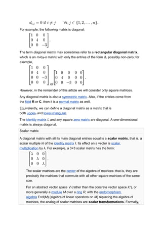


![If a random variable X has the expected value (mean) μ = E[X], then the variance
of X is given by:
This definition encompasses random variables that are discrete, continuous, or
neither. It can be expanded as follows:
The variance of random variable X is typically designated as Var(X), , or simply
σ2
(pronounced “sigma squared”). If a distribution does not have an expected value,
as is the case for the Cauchy distribution, it does not have a variance either. Many
other distributions for which the expected value does exist do not have a finite
variance because the relevant integral diverges. An example is a Pareto
distribution whose index k satisfies 1 < k ≤ 2.
[edit]Continuous case
If the random variable X is continuous with probability density function f(x),
where
and where the integrals are definite integrals taken for x ranging over the range of X.
[edit]Discrete case
If the random variable X is discrete with probability mass function x1 ↦ p1, ..., xn ↦ pn,
then](https://image.slidesharecdn.com/1561-maths-161031144107/85/1561-maths-109-320.jpg)
![where
.
(When such a discrete weighted variance is specified by weights whose sum is
not 1, then one divides by the sum of the weights.) That is, it is the expected value of
the square of the deviation of X from its own mean. In plain language, it can be
expressed as “The mean of the square of the deviation of each data point from the
average”. It is thus the mean squared deviation.
Examples
Exponential distribution
The exponential distribution with parameter λ is a continuous distribution whose
support is the semi-infinite interval [0,∞). Its probability density function is given by:
and it has expected value μ = λ−1
. Therefore the variance is equal to:
So for an exponentially distributed random variable σ2
= μ2
.
[edit]Fair dice
A six-sided fair die can be modelled with a discrete random variable with outcomes 1
through 6, each with equal probability 1
/6. The expected value is
(1 + 2 + 3 + 4 + 5 + 6)/6 = 3.5. Therefore the variance can be computed to be:
Properties
Variance is non-negative because the squares are positive or zero. The variance of
a constant random variable is zero, and the variance of a variable in a data set is 0 if
and only if all entries have the same value.
Variance is invariant with respect to changes in a location parameter. That is, if a
constant is added to all values of the variable, the variance is unchanged. If all
values are scaled by a constant, the variance is scaled by the square of that
constant. These two properties can be expressed in the following formula:](https://image.slidesharecdn.com/1561-maths-161031144107/85/1561-maths-110-320.jpg)

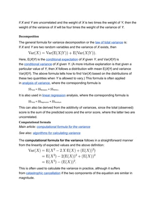
![1 + 2 × 2 + 3 × 3 + 4 × 4) / 4 = 7.5. The regular mean of all four numbers is 2.5, so
the square of the mean is 6.25. Therefore the variance is 7.5 − 6.25 = 1.25, which is
indeed the same result obtained earlier with the definition formulas. Many pocket
calculators use an algorithm that is based on this formula and that allows them to
compute the variance while the data are entered, without storing all values in
memory. The algorithm is to adjust only three variables when a new data value is
entered: The number of data entered so far (n), the sum of the values so far (S), and
the sum of the squared values so far (SS). For example, if the data are 1, 2, 3, 4,
then after entering the first value, the algorithm would have n = 1, S = 1 and SS = 1.
After entering the second value (2), it would have n = 2, S = 3 and SS = 5. When all
data are entered, it would have n = 4, S = 10 and SS = 30. Next, the mean is
computed as M = S / n, and finally the variance is computed as SS / n − M × M. In
this example the outcome would be 30 / 4 − 2.5 × 2.5 = 7.5 − 6.25 = 1.25. If the
unbiased sample estimate is to be computed, the outcome will be multiplied by n /
(n − 1), which yields 1.667 in this example.
Sum of uncorrelated variables (Bienaymé formula)
One reason for the use of the variance in preference to other measures of dispersion
is that the variance of the sum (or the difference) of uncorrelated random variables is
the sum of their variances:
This statement is called the Bienaymé formula.[1]
and was discovered in 1853. It is
often made with the stronger condition that the variables are independent, but
uncorrelatedness suffices. So if all the variables have the same variance σ2
, then,
since division by n is a linear transformation, this formula immediately implies that
the variance of their mean is
That is, the variance of the mean decreases when n increases. This formula for the
variance of the mean is used in the definition of the standard error of the sample
mean, which is used in the central limit theorem.
[edit]Sum of correlated variables
In general, if the variables are correlated, then the variance of their sum is the sum of
their covariances:](https://image.slidesharecdn.com/1561-maths-161031144107/85/1561-maths-112-320.jpg)
![(Note: This by definition includes the variance of each variable, since
Cov(X,X) = Var(X).)
Here Cov is the covariance, which is zero for independent random variables (if it
exists). The formula states that the variance of a sum is equal to the sum of all
elements in the covariance matrix of the components. This formula is used in the
theory of Cronbach's alpha in classical test theory.
So if the variables have equal variance σ2
and the average correlation of distinct
variables is ρ, then the variance of their mean is
This implies that the variance of the mean increases with the average of the
correlations. Moreover, if the variables have unit variance, for example if they are
standardized, then this simplifies to
This formula is used in the Spearman-Brown prediction formula of classical test
theory. This converges to ρ if n goes to infinity, provided that the average correlation
remains constant or converges too. So for the variance of the mean of standardized
variables with equal correlations or converging average correlation we have
Therefore, the variance of the mean of a large number of standardized variables is
approximately equal to their average correlation. This makes clear that the sample
mean of correlated variables does generally not converge to the population mean,
even though the Law of large numbers states that the sample mean will converge for
independent variables.
[edit]Weighted sum of variables
The scaling property and the Bienaymé formula, along with this property from
the covariance page: Cov(aX, bY) = ab Cov(X, Y) jointly imply that
This implies that in a weighted sum of variables, the variable with the largest weight
will have a disproportionally large weight in the variance of the total. For example,](https://image.slidesharecdn.com/1561-maths-161031144107/85/1561-maths-113-320.jpg)
![Characteristic property
The second moment of a random variable attains the minimum value when taken
around the first moment (i.e., mean) of the random variable,
i.e. . Conversely, if a continuous function
satisfies for all random variables X, then it is
necessarily of the form , where a > 0. This also holds in the
multidimensional case.[2]
[edit]Calculation from the CDF
The population variance for a non-negative random variable can be expressed in
terms of the cumulative distribution function F using
where H(u) = 1 − F(u) is the right tail function. This expression can be used to
calculate the variance in situations where the CDF, but not the density, can be
conveniently expressed.
[edit]Approximating the variance of a function
The delta method uses second-order Taylor expansions to approximate the variance
of a function of one or more random variables: see Taylor expansions for the
moments of functions of random variables. For example, the approximate variance of
a function of one variable is given by
provided that f is twice differentiable and that the mean and variance of X are finite.
[citation needed]
[edit]Population variance and sample variance
In general, the population variance of a finite population of size N is given by
where
is the population mean.
In many practical situations, the true variance of a population is not known a
priori and must be computed somehow. When dealing with extremely large
populations, it is not possible to count every object in the population.](https://image.slidesharecdn.com/1561-maths-161031144107/85/1561-maths-115-320.jpg)
![A common task is to estimate the variance of a population from a sample.[3]
We take
a sample with replacement of n values y1, ..., yn from the population, where n < N,
and estimate the variance on the basis of this sample. There are several good
estimators. Two of them are well known:
and
[4]
Both are referred to as sample variance. Here,
denotes the sample mean:
The two estimators only differ slightly as can be seen, and for larger values of
the sample size n the difference is negligible. While the first one may be seen as the
variance of the sample considered as a population, the second one is the unbiased
estimator of the population variance, meaning that its expected value E[s2
] is equal
to the true variance of the sampled random variable; the use of the term n − 1 is
called Bessel's correction. The sample variance with n − 1 is a U-statistic for the
function ƒ(x1, x2) = (x1 − x2)2
/2, meaning that it is obtained by averaging a 2-sample
statistic over 2-element subsets of the population.](https://image.slidesharecdn.com/1561-maths-161031144107/85/1561-maths-116-320.jpg)

![[edit]Generalizations
If X is a vector-valued random variable, with values in , and thought of as a
column vector, then the natural generalization of variance
is , where and is the transpose of X, and
so is a row vector. This variance is a positive semi-definite square matrix, commonly
referred to as the covariance matrix.
If X is a complex-valued random variable, with values in , then its variance
is , where is the conjugate transpose of X. This variance
is also a positive semi-definite square matrix.
[edit]History
The term variance was first introduced by Ronald Fisher in his 1918 paper The
Correlation Between Relatives on the Supposition of Mendelian Inheritance:[5]
The great body of available statistics show us that the deviations of a human
measurement from its mean follow very closely the Normal Law of Errors, and,
therefore, that the variability may be uniformly measured by the standard
deviation corresponding to the square root of the mean square error. When there are
two independent causes of variability capable of producing in an otherwise uniform
population distributions with standard deviations θ1 and θ2, it is found that the
distribution, when both causes act together, has a standard deviation . It is
therefore desirable in analysing the causes of variability to deal with the square of
the standard deviation as the measure of variability. We shall term this quantity the
Variance...
[edit]Moment of inertia
The variance of a probability distribution is analogous to the moment of
inertia in classical mechanics of a corresponding mass distribution along a line, with
respect to rotation about its center of mass. It is because of this analogy that such
things as the variance are called moments of probability distributions. The
covariance matrix is related to the moment of inertia tensor for multivariate
distributions. The moment of inertia of a cloud of n points with a covariance matrix
of Σ is given by
This difference between moment of inertia in physics and in statistics is clear for
points that are gathered along a line. Suppose many points are close to the x and
distributed along it. The covariance matrix might look like](https://image.slidesharecdn.com/1561-maths-161031144107/85/1561-maths-118-320.jpg)

![The moment of inertia has two forms, a scalar form, I, (used when the axis of rotation
is specified) and a more general tensor form that does not require the axis of rotation
to be specified. The scalar moment of inertia, I, (often called simply the "moment of
inertia") allows a succinct analysis of many simple problems inrotational dynamics,
such as objects rolling down inclines and the behavior of pulleys. For instance, while
a block of any shape will slide down a frictionless decline at the same rate, rolling
objects may descend at different rates, depending on their moments of inertia. A
hoop will descend more slowly than a solid disk of equal mass and radius because
more of its mass is located far from the axis of rotation, and thus needs to move
faster if the hoop rolls at the same angular velocity. However, for (more complicated)
problems in which the axis of rotation can change, the scalar treatment is
inadequate, and the tensor treatment must be used (although shortcuts are possible
in special situations). Examples requiring such a treatment include gyroscopes, tops,
and even satellites, all objects whose alignment can change.
The moment of inertia is also called the mass moment of inertia (especially by
mechanical engineers) to avoid confusion with the second moment of area, which is
sometimes called the moment of inertia (especially by structural engineers). The
easiest way to differentiate these quantities is through their units (kg·m2
as opposed
to m4
). In addition, moment of inertia should not be confused with polar moment of
inertia, which is a measure of an object's ability to resist torsion (twisting) only.
[edit]Scalar moment of inertia
[edit]Definition
A simple definition of the moment of inertia (with respect to a given axis of rotation)
of any object, be it a point mass or a 3D-structure, is given by:
where m is mass and r is the perpendicular distance to the axis of rotation.
[edit]Detailed analysis
The (scalar) moment of inertia of a point mass rotating about a known axis is defined
by
The moment of inertia is additive. Thus, for a rigid body consisting of N point
masses mi with distances ri to the rotation axis, the total moment of inertia equals the
sum of the point-mass moments of inertia:](https://image.slidesharecdn.com/1561-maths-161031144107/85/1561-maths-120-320.jpg)

![c = 1/2, solid cylinder or disk around its center.
When c is 1, the length (L) is called the radius of gyration.
For more examples, see the List of moments of inertia.
[Parallel axis theorem
Main article: Parallel axis theorem
Once the moment of inertia has been calculated for rotations about the center of
mass of a rigid body, one can conveniently recalculate the moment of inertia for all
parallel rotation axes as well, without having to resort to the formal definition. If the
axis of rotation is displaced by a distance r from the center of mass axis of rotation
(e.g., spinning a disc about a point on its periphery, rather than through its center,)
the displaced and center-moment of inertia are related as follows:
This theorem is also known as the parallel axes rule and is a special case
of Steiner's parallel-axis theorem.
Composite bodies
If a body can be decomposed (either physically or conceptually) into several
constituent parts, then the moment of inertia of the body about a given axis is
obtained by summing the moments of inertia of each constituent part around the
same given axis.[2]
Equations involving the moment of inertia
The rotational kinetic energy of a rigid body can be expressed in terms of its moment
of inertia. For a system with N point masses mi moving with speeds vi, the rotational
kinetic energy T equals
where ω is the common angular velocity (in radians per second). The final
expression I ω2
/ 2 also holds for a mass density function with a generalization of the
above derivation from a discrete summation to an integration.
In the special case where the angular momentum vector is parallel to the angular
velocity vector, one can relate them by the equation
where L is the angular momentum and ω is the angular velocity. However, this
equation does not hold in many cases of interest, such as the torque-](https://image.slidesharecdn.com/1561-maths-161031144107/85/1561-maths-122-320.jpg)
![free precession of a rotating object, although its more general tensor form is always
correct.
When the moment of inertia is constant, one can also relate the torque on an object
and its angular acceleration in a similar equation:
where τ is the torque and α is the angular acceleration.
Moment of inertia tensor
In three dimensions, if the axis of rotation is not given, we need to be able to
generalize the scalar moment of inertia to a quantity that allows us to compute a
moment of inertia about arbitrary axes. This quantity is known as the moment of
inertia tensor and can be represented as a symmetric positive semi-definite
matrix, I. This representation elegantly generalizes the scalar case: The angular
momentum vector, is related to the rotation velocity vector, ω by
and the kinetic energy is given by
as compared with
in the scalar case.
Like the scalar moment of inertia, the moment of inertia tensor may be calculated
with respect to any point in space, but for practical purposes, the center of mass is
almost always used.
[edit]Definition
For a rigid object of N point masses mk, the moment of inertia tensor is given by
,
where](https://image.slidesharecdn.com/1561-maths-161031144107/85/1561-maths-123-320.jpg)

![is This is a quadratic form in and, after a bit
more algebra, this leads to a tensor formula for the moment of inertia
.
This is exactly the formula given below for the moment of inertia in the case of a
single particle. For multiple particles we need only recall that the moment of inertia is
additive in order to see that this formula is correct.
Reduction to scalar
For any axis , represented as a column vector with elements ni, the scalar
form I can be calculated from the tensor form I as
The range of both summations correspond to the three Cartesian coordinates.
The following equivalent expression avoids the use of transposed vectors which
are not supported in maths libraries because internally vectors and their
transpose are stored as the same linear array,
However it should be noted that although this equation is mathematically
equivalent to the equation above for any matrix, inertia tensors are
symmetrical. This means that it can be further simplified to:
[edit]Principal axes of inertia
By the spectral theorem, since the moment of inertia tensor is real and symmetric, it
is possible to find a Cartesian coordinate system in which it is diagonal, having the
form
where the coordinate axes are called the principal axes and the
constants I1, I2 and I3 are called the principal moments of inertia. The principal
axes of a body, therefore, are a cartesian coordinate system whose origin is located
at the center of mass. [3]
The unit vectors along the principal axes are usually
denoted as (e1, e2, e3). This result was first shown by J. J. Sylvester (1852), and is a](https://image.slidesharecdn.com/1561-maths-161031144107/85/1561-maths-125-320.jpg)
![form ofSylvester's law of inertia. The principal axis with the highest moment of inertia
is sometimes called the figure axis or axis of figure.
When all principal moments of inertia are distinct, the principal axes are uniquely
specified. If two principal moments are the same, the rigid body is called
a symmetrical top and there is no unique choice for the two corresponding principal
axes. If all three principal moments are the same, the rigid body is called a spherical
top (although it need not be spherical) and any axis can be considered a principal
axis, meaning that the moment of inertia is the same about any axis.
The principal axes are often aligned with the object's symmetry axes. If a rigid body
has an axis of symmetry of order m, i.e., is symmetrical under rotations of
360°/m about a given axis, the symmetry axis is a principal axis. When m > 2, the
rigid body is a symmetrical top. If a rigid body has at least two symmetry axes that
are not parallel or perpendicular to each other, it is a spherical top, e.g., a cube or
any other Platonic solid.
The motion of vehicles is often described about these axes with
the rotations called yaw, pitch, and roll.
A practical example of this mathematical phenomenon is the routine automotive task
of balancing a tire, which basically means adjusting the distribution of mass of a car
wheel such that its principal axis of inertia is aligned with the axle so the wheel does
not wobble.
[edit]Parallel axis theorem
Once the moment of inertia tensor has been calculated for rotations about the center
of mass of the rigid body, there is a useful labor-saving method to compute the
tensor for rotations offset from the center of mass.
If the axis of rotation is displaced by a vector R from the center of mass, the new
moment of inertia tensor equals
where m is the total mass of the rigid body, E3 is the 3 × 3 identity matrix, and is
the outer product.
[edit]Rotational symmetry
Using the above equation to express all moments of inertia in terms of integrals of
variables either along or perpendicular to the axis of symmetry usually simplifies the
calculation of these moments considerably.
Comparison with covariance matrix
Main article: Moment (mathematics)](https://image.slidesharecdn.com/1561-maths-161031144107/85/1561-maths-126-320.jpg)
![The moment of inertia tensor about the center of mass of a 3 dimensional rigid body
is related to the covariance matrix of a trivariate random vector whose probability
density function is proportional to the pointwise density of the rigid body by:[citation needed]
where n is the number of points.
The structure of the moment-of-inertia tensor comes from the fact that it is to be used
as a bilinear form on rotation vectors in the form
Each element of mass has a kinetic energy of
The velocity of each element of mass is where r is a vector from the center of
rotation to that element of mass. The cross product can be converted to matrix
multiplication so that
and similarly
Thus,
plugging in the definition of the term leads directly to the structure of the
moment tensor.](https://image.slidesharecdn.com/1561-maths-161031144107/85/1561-maths-127-320.jpg)

The document explains the concepts of arithmetic mean and geometric mean, outlining how to calculate each and the contexts in which they are used. It highlights that the arithmetic mean is the average computed by summing values and dividing by the count, while the geometric mean is the nth root of the product of values, applicable primarily for positive numbers. It also discusses the importance of using the geometric mean for calculating investment returns due to their interdependent nature.