The document provides an overview of matrix algebra operations in R, including vectors, matrices, and their applications in psychological data analysis. It covers vector operations like addition, multiplication, and combining vectors into matrices. Matrix topics include addition, multiplication, finding the diagonal, identity matrices, and inversion. The document also demonstrates how these operations can be used for data manipulation tasks like calculating statistics, finding test reliability, and multiple correlation analyses.

1. Matrix Algebra in R
William Revelle
Northwestern University
January 24, 2007
Prepared as part of a course on Latent Variable Modeling, Winter, 2007
and as a supplement to the Guide to R for psychologists.
email comments to: revelle@northwestern.edu
A Matrix Algebra in R 2
A.1 Vectors . . . . . . . . . . . . . . . . . . . . . . . . . . . . . . . . . . . . . . . . 2
A.1.1 Vector multiplication . . . . . . . . . . . . . . . . . . . . . . . . . . . . . 3
A.1.2 Simple statistics using vectors . . . . . . . . . . . . . . . . . . . . . . . . 5
A.1.3 Combining vectors . . . . . . . . . . . . . . . . . . . . . . . . . . . . . . 7
A.2 Matrices . . . . . . . . . . . . . . . . . . . . . . . . . . . . . . . . . . . . . . . . 8
A.2.1 Matrix addition . . . . . . . . . . . . . . . . . . . . . . . . . . . . . . . . 9
A.2.2 Matrix multiplication . . . . . . . . . . . . . . . . . . . . . . . . . . . . 10
A.2.3 Finding and using the diagonal . . . . . . . . . . . . . . . . . . . . . . . 12
A.2.4 The Identity Matrix . . . . . . . . . . . . . . . . . . . . . . . . . . . . . 13
A.2.5 Matrix Inversion . . . . . . . . . . . . . . . . . . . . . . . . . . . . . . . 13
A.3 Matrix operations for data manipulation . . . . . . . . . . . . . . . . . . . . . . 14
A.3.1 Matrix operations on the raw data . . . . . . . . . . . . . . . . . . . . . 16
A.3.2 Matrix operations on the correlation matrix . . . . . . . . . . . . . . . . 16
A.3.3 Using matrices to find test reliability . . . . . . . . . . . . . . . . . . . . 17
A.4 Multiple correlation . . . . . . . . . . . . . . . . . . . . . . . . . . . . . . . . . 18
A.4.1 Data level analyses . . . . . . . . . . . . . . . . . . . . . . . . . . . . . . 19
A.4.2 Non optimal weights and the goodness of fit . . . . . . . . . . . . . . . . 21
1

2. Appendix A
Matrix Algebra in R
Much of psychometrics in particular, and psychological data analysis in general consists of
operations on vectors and matrices. This appendix offers a quick review of matrix oper-
ations with a particular emphasis upon how to do matrix operations in R. For more in-
formation on how to use R, consult the short guide to R for psychologists (at http://
personality-project.org/r/r.guide.html) or the even shorter guide at personality-project.
org/r/r.205.tutorial.html.
A.1 Vectors
A vector is a one dimensional array of n numbers. Basic operations on a vector are addition
and subtraction. Multiplication is somewhat more complicated, for the order in which two
vectors are multiplied changes the result. That is AB 6= BA.
Consider V1 = the first 10 integers, and V2 = the next 10 integers:
> V1 <- as.vector(seq(1, 10))
[1] 1 2 3 4 5 6 7 8 9 10
> V2 <- as.vector(seq(11, 20))
[1] 11 12 13 14 15 16 17 18 19 20
We can add a constant to each element in a vector
> V4 <- V1 + 20
[1] 21 22 23 24 25 26 27 28 29 30
or we can add each element of the first vector to the corresponding element of the second
vector
> V3 <- V1 + V2
[1] 12 14 16 18 20 22 24 26 28 30
2

3. Strangely enough, a vector in R is dimensionless, but it has a length. If we want to multiply
two vectors, we first need to think of the vector either as row or as a column. A column
vector can be made into a row vector (and vice versa) by the transpose operation. While a
vector has no dimensions, the transpose of a vector is two dimensional! It is a matrix with
with 1 row and n columns. (Although the dim command will return no dimensions, in terms
of multiplication, a vector is a matrix of n rows and 1 column.)
Consider the following:
> dim(V1)
NULL
> length(V1)
[1] 10
> dim(t(V1))
[1] 1 10
> dim(t(t(V1)))
[1] 10 1
> TV <- t(V1)
[,1] [,2] [,3] [,4] [,5] [,6] [,7] [,8] [,9] [,10]
[1,] 1 2 3 4 5 6 7 8 9 10
> t(TV)
[,1]
[1,] 1
[2,] 2
[3,] 3
[4,] 4
[5,] 5
[6,] 6
[7,] 7
[8,] 8
[9,] 9
[10,] 10
A.1.1 Vector multiplication
Just as we can add a number to every element in a vector, so can we multiply a number
(a“scaler”) by every element in a vector.
> V2 <- 4 * V1
[1] 4 8 12 16 20 24 28 32 36 40
3

4. There are three types of multiplication of vectors in R. Simple multiplication (each term in
one vector is multiplied by its corresponding term in the other vector), as well as the inner
and outer products of two vectors.
Simple multiplication requires that each vector be of the same length. Using the V1 and V2
vectors from before, we can find the 10 products of their elements:
> V1
[1] 1 2 3 4 5 6 7 8 9 10
> V2
[1] 4 8 12 16 20 24 28 32 36 40
> V1 * V2
[1] 4 16 36 64 100 144 196 256 324 400
The “outer product” of a n * 1 element vector with a 1 * m element vector will result in a n
* m element matrix. (The dimension of the resulting product is the outer dimensions of the
two vectors in the multiplication). The vector multiply operator is %*%. In the following
equation, the subscripts refer to the dimensions of the variable.
nX1 ∗1 Ym =n (XY )m (A.1)
> V1 <- seq(1, 10)
> V2 <- seq(1, 4)
> V1
[1] 1 2 3 4 5 6 7 8 9 10
> V2
[1] 1 2 3 4
> outer.prod <- V1 %*% t(V2)
> outer.prod
[,1] [,2] [,3] [,4]
[1,] 1 2 3 4
[2,] 2 4 6 8
[3,] 3 6 9 12
[4,] 4 8 12 16
[5,] 5 10 15 20
[6,] 6 12 18 24
[7,] 7 14 21 28
[8,] 8 16 24 32
[9,] 9 18 27 36
[10,] 10 20 30 40
The outer product of the first ten integers is, of course, the multiplication table known to all
elementary school students:
4

5. > outer.prod <- V1 %*% t(V1)
[,1] [,2] [,3] [,4] [,5] [,6] [,7] [,8] [,9] [,10]
[1,] 1 2 3 4 5 6 7 8 9 10
[2,] 2 4 6 8 10 12 14 16 18 20
[3,] 3 6 9 12 15 18 21 24 27 30
[4,] 4 8 12 16 20 24 28 32 36 40
[5,] 5 10 15 20 25 30 35 40 45 50
[6,] 6 12 18 24 30 36 42 48 54 60
[7,] 7 14 21 28 35 42 49 56 63 70
[8,] 8 16 24 32 40 48 56 64 72 80
[9,] 9 18 27 36 45 54 63 72 81 90
[10,] 10 20 30 40 50 60 70 80 90 100
The “inner product” is perhaps a more useful operation, for it not only multiplies each corre-
sponding element of two vectors, but also sums the resulting product:
inner.product =
N
X
i=1
V 1i ∗ V 2i (A.2)
> V1 <- seq(1, 10)
> V2 <- seq(11, 20)
> V1
[1] 1 2 3 4 5 6 7 8 9 10
> V2
[1] 11 12 13 14 15 16 17 18 19 20
> in.prod <- t(V1) %*% V2
> in.prod
[,1]
[1,] 935
Note that the inner product of two vectors is of length =1 but is a matrix with 1 row and 1
column. (This is the dimension of the inner dimensions (1) of the two vectors.)
A.1.2 Simple statistics using vectors
Although there are built in functions in R to do most of our statistics, it is useful to understand
how these operations can be done using vector and matrix operations. Here we consider how
to find the mean of a vector, remove it from all the numbers, and then find the average
squared deviation from the mean (the variance).
Consider the mean of all numbers in a vector. To find this we just need to add up the numbers
(the inner product of the vector with a vector of 1’s) and then divide by n (multiply by the
scaler 1/n). First we create a vector of 1s by using the repeat operation. We then show three
different equations for the mean.V, all of which are equivalent.
5

6. > V <- V1
[1] 1 2 3 4 5 6 7 8 9 10
> one <- rep(1, length(V))
[1] 1 1 1 1 1 1 1 1 1 1
> sum.V <- t(one) %*% V
[,1]
[1,] 55
> mean.V <- sum.V * (1/length(V))
[,1]
[1,] 5.5
> mean.V <- t(one) %*% V * (1/length(V))
[,1]
[1,] 5.5
> mean.V <- t(one) %*% V/length(V)
[,1]
[1,] 5.5
The variance is the average squared deviation from the mean. To find the variance, we first
find deviation scores by subtracting the mean from each value of the vector. Then, to find
the sum of the squared deviations take the inner product of the result with itself. This Sum
of Squares becomes a variance if we divide by the degrees of freedom (n-1) to get an unbiased
estimate of the population variance). First we find the mean centered vector:
> V - mean.V
[1] -4.5 -3.5 -2.5 -1.5 -0.5 0.5 1.5 2.5 3.5 4.5
And then we find the variance as the mean square by taking the inner product:
> Var.V <- t(V - mean.V) %*% (V - mean.V) * (1/(length(V) - 1))
[,1]
[1,] 9.166667
Compare these results with the more typical scale, mean and var operations:
> scale(V, scale = FALSE)
[,1]
[1,] -4.5
[2,] -3.5
[3,] -2.5
[4,] -1.5
[5,] -0.5
[6,] 0.5
[7,] 1.5
6

7. [8,] 2.5
[9,] 3.5
[10,] 4.5
attr(,"scaled:center")
[1] 5.5
> mean(V)
[1] 5.5
> var(V)
[1] 9.166667
A.1.3 Combining vectors
We can form more complex data structures than vectors by combining the vectors, either by
columns (cbind) or by rows (rbind). The resulting data structure is a matrix.
> Xc <- cbind(V1, V2, V3)
V1 V2 V3
[1,] 1 11 12
[2,] 2 12 14
[3,] 3 13 16
[4,] 4 14 18
[5,] 5 15 20
[6,] 6 16 22
[7,] 7 17 24
[8,] 8 18 26
[9,] 9 19 28
[10,] 10 20 30
> Xr <- rbind(V1, V2, V3)
[,1] [,2] [,3] [,4] [,5] [,6] [,7] [,8] [,9] [,10]
V1 1 2 3 4 5 6 7 8 9 10
V2 11 12 13 14 15 16 17 18 19 20
V3 12 14 16 18 20 22 24 26 28 30
> dim(Xc)
[1] 10 3
> dim(Xr)
[1] 3 10
7

8. A.2 Matrices
A matrix is just a two dimensional (rectangular) organization of numbers. It is a vector of
vectors. For data analysis, the typical data matrix is organized with columns representing
different variables and rows containing the responses of a particular subject. Thus, a 10 x
4 data matrix (10 rows, 4 columns) would contain the data of 10 subjects on 4 different
variables. Note that the matrix operation has taken the numbers 1 through 40 and organized
them column wise. That is, a matrix is just a way (and a very convenient one at that) of
organizing a vector.
R provides numeric row and column names (e.g., [1,] is the first row, [,4] is the fourth column,
but it is useful to label the rows and columns to make the rows (subjects) and columns
(variables) distinction more obvious. 1
> Xij <- matrix(seq(1:40), ncol = 4)
> rownames(Xij) <- paste("S", seq(1, dim(Xij)[1]), sep = "")
> colnames(Xij) <- paste("V", seq(1, dim(Xij)[2]), sep = "")
> Xij
V1 V2 V3 V4
S1 1 11 21 31
S2 2 12 22 32
S3 3 13 23 33
S4 4 14 24 34
S5 5 15 25 35
S6 6 16 26 36
S7 7 17 27 37
S8 8 18 28 38
S9 9 19 29 39
S10 10 20 30 40
Just as the transpose of a vector makes a column vector into a row vector, so does the
transpose of a matrix swap the rows for the columns. Note that now the subjects are columns
and the variables are the rows.
> t(Xij)
S1 S2 S3 S4 S5 S6 S7 S8 S9 S10
V1 1 2 3 4 5 6 7 8 9 10
V2 11 12 13 14 15 16 17 18 19 20
V3 21 22 23 24 25 26 27 28 29 30
V4 31 32 33 34 35 36 37 38 39 40
1
Although many think of matrices as developed in the 17th century, O’Conner and Robertson discuss the
history of matrix algebra back to the Babylonians (http://www-history.mcs.st-andrews.ac.uk/history/
HistTopics/Matrices_and_determinants.html)
8

9. A.2.1 Matrix addition
The previous matrix is rather uninteresting, in that all the columns are simple products of
the first column. A more typical matrix might be formed by sampling from the digits 0-9.
For the purpose of this demonstration, we will set the random number seed to a memorable
number so that it will yield the same answer each time.
> set.seed(42)
> Xij <- matrix(sample(seq(0, 9), 40, replace = TRUE), ncol = 4)
> rownames(Xij) <- paste("S", seq(1, dim(Xij)[1]), sep = "")
> colnames(Xij) <- paste("V", seq(1, dim(Xij)[2]), sep = "")
> print(Xij)
V1 V2 V3 V4
S1 9 4 9 7
S2 9 7 1 8
S3 2 9 9 3
S4 8 2 9 6
S5 6 4 0 0
S6 5 9 5 8
S7 7 9 3 0
S8 1 1 9 2
S9 6 4 4 9
S10 7 5 8 6
Just as we could with vectors, we can add, subtract, muliply or divide the matrix by a scaler
(a number with out a dimension).
> Xij + 4
V1 V2 V3 V4
S1 13 8 13 11
S2 13 11 5 12
S3 6 13 13 7
S4 12 6 13 10
S5 10 8 4 4
S6 9 13 9 12
S7 11 13 7 4
S8 5 5 13 6
S9 10 8 8 13
S10 11 9 12 10
> round((Xij + 4)/3, 2)
V1 V2 V3 V4
S1 4.33 2.67 4.33 3.67
S2 4.33 3.67 1.67 4.00
S3 2.00 4.33 4.33 2.33
S4 4.00 2.00 4.33 3.33
S5 3.33 2.67 1.33 1.33
9

10. S6 3.00 4.33 3.00 4.00
S7 3.67 4.33 2.33 1.33
S8 1.67 1.67 4.33 2.00
S9 3.33 2.67 2.67 4.33
S10 3.67 3.00 4.00 3.33
We can also multiply each row (or column, depending upon order) by a vector.
> V
[1] 1 2 3 4 5 6 7 8 9 10
> Xij * V
V1 V2 V3 V4
S1 9 4 9 7
S2 18 14 2 16
S3 6 27 27 9
S4 32 8 36 24
S5 30 20 0 0
S6 30 54 30 48
S7 49 63 21 0
S8 8 8 72 16
S9 54 36 36 81
S10 70 50 80 60
A.2.2 Matrix multiplication
Matrix multiplication is a combination of multiplication and addition. For a matrix mXn of
dimensions m*n and nYp of dimension n * p, the product, mXYp is a m * p matrix where each
element is the sum of the products of the rows of the first and the columns of the second.
That is, the matrix mXYp has elements xyij where each
xyij =
n
X
k=1
xik ∗ yjk (A.3)
Consider our matrix Xij with 10 rows of 4 columns. Call an individual element in this matrix
xij. We can find the sums for each column of the matrix by multiplying the matrix by our
“one” vector with Xij. That is, we can find
PN
i=1 Xij for the j columns, and then divide by the
number (n) of rows. (Note that we can get the same result by finding colMeans(Xij).
We can use the dim function to find out how many cases (the number of rows) or the number
of variables (number of columns). dim has two elements: dim(Xij)[1] = number of rows,
dim(Xij)[2] is the number of columns.
> dim(Xij)
[1] 10 4
> n <- dim(Xij)[1]
10

11. [1] 10
> one <- rep(1, n)
[1] 1 1 1 1 1 1 1 1 1 1
> X.means <- t(one) %*% Xij/n
V1 V2 V3 V4
[1,] 6 5.4 5.7 4.9
A built in function to find the means of the columns is colMeans. (See rowMeans for the
equivalent for rows.)
> colMeans(Xij)
V1 V2 V3 V4
6.0 5.4 5.7 4.9
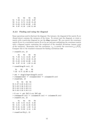
Variances and covariances are measures of dispersion around the mean. We find these by first
subtracting the means from all the observations. This means centered matrix is the original
matrix minus a matrix of means. To make them have the same dimensions we premultiply
the means vector by a vector of ones and subtract this from the data matrix.
> X.diff <- Xij - one %*% X.means
V1 V2 V3 V4
S1 3 -1.4 3.3 2.1
S2 3 1.6 -4.7 3.1
S3 -4 3.6 3.3 -1.9
S4 2 -3.4 3.3 1.1
S5 0 -1.4 -5.7 -4.9
S6 -1 3.6 -0.7 3.1
S7 1 3.6 -2.7 -4.9
S8 -5 -4.4 3.3 -2.9
S9 0 -1.4 -1.7 4.1
S10 1 -0.4 2.3 1.1
To find the variance/covariance matrix, we can first find the the inner product of the means
centered matrix X.diff = Xij - X.means t(Xij-X.means) with itself and divide by n-1. We
can compare this result to the result of the cov function (the normal way to find covari-
ances).
> X.cov <- t(X.diff) %*% X.diff/(n - 1)
> round(X.cov, 2)
V1 V2 V3 V4
V1 7.33 0.11 -3.00 3.67
V2 0.11 8.71 -3.20 -0.18
V3 -3.00 -3.20 12.68 1.63
V4 3.67 -0.18 1.63 11.43
> round(cov(Xij), 2)
11

12. V1 V2 V3 V4
V1 7.33 0.11 -3.00 3.67
V2 0.11 8.71 -3.20 -0.18
V3 -3.00 -3.20 12.68 1.63
V4 3.67 -0.18 1.63 11.43
A.2.3 Finding and using the diagonal
Some operations need to find just the diagonal. For instance, the diagonal of the matrix X.cov
(found above) contains the variances of the items. To extract just the diagonal, or create a
matrix with a particular diagonal we use the diag command. We can convert the covariance
matrix X.cov to a correlation matrix X.cor by pre and post multiplying the covariance matrix
with a diagonal matrix containing the reciprocal of the standard deviations (square roots
of the variances). Remember that the correlation, rxy, is merely the covariancexy/
p
VxVy.
Compare this to the standard command for finding correlations cor.
> round(X.cov, 2)
V1 V2 V3 V4
V1 7.33 0.11 -3.00 3.67
V2 0.11 8.71 -3.20 -0.18
V3 -3.00 -3.20 12.68 1.63
V4 3.67 -0.18 1.63 11.43
> round(diag(X.cov), 2)
V1 V2 V3 V4
7.33 8.71 12.68 11.43
> sdi <- diag(1/sqrt(diag(X.cov)))
> rownames(sdi) <- colnames(sdi) <- colnames(X.cov)
> round(sdi, 2)
V1 V2 V3 V4
V1 0.37 0.00 0.00 0.0
V2 0.00 0.34 0.00 0.0
V3 0.00 0.00 0.28 0.0
V4 0.00 0.00 0.00 0.3
> X.cor <- sdi %*% X.cov %*% sdi
> rownames(X.cor) <- colnames(X.cor) <- colnames(X.cov)
> round(X.cor, 2)
V1 V2 V3 V4
V1 1.00 0.01 -0.31 0.40
V2 0.01 1.00 -0.30 -0.02
V3 -0.31 -0.30 1.00 0.14
V4 0.40 -0.02 0.14 1.00
> round(cor(Xij), 2)
12

13. V1 V2 V3 V4
V1 1.00 0.01 -0.31 0.40
V2 0.01 1.00 -0.30 -0.02
V3 -0.31 -0.30 1.00 0.14
V4 0.40 -0.02 0.14 1.00
A.2.4 The Identity Matrix
The identity matrix is merely that matrix, which when multiplied by another matrix, yields
the other matrix. (The equivalent of 1 in normal arithmetic.) It is a diagonal matrix with 1
on the diagonal I <- diag(1,nrow=dim(X.cov)[1],ncol=dim(X.cov)[2])
A.2.5 Matrix Inversion
The inverse of a square matrix is the matrix equivalent of dividing by that matrix. That
is, either pre or post multiplying a matrix by its inverse yields the identity matrix. The
inverse is particularly important in multiple regression, for it allows is to solve for the beta
weights.
Given the equation
Y = bX + c (A.4)
we can solve for b by multiplying both sides of the equation by
X−1
orY X−1
= bXX−1
= b (A.5)
We can find the inverse by using the solve function. To show that XX−1 = X−1X = I, we
do the multiplication.
> X.inv <- solve(X.cov)
V1 V2 V3 V4
V1 0.19638636 0.01817060 0.06024476 -0.07130491
V2 0.01817060 0.12828756 0.03787166 -0.00924279
V3 0.06024476 0.03787166 0.10707738 -0.03402838
V4 -0.07130491 -0.00924279 -0.03402838 0.11504850
> round(X.cov %*% X.inv, 2)
V1 V2 V3 V4
V1 1 0 0 0
V2 0 1 0 0
V3 0 0 1 0
V4 0 0 0 1
> round(X.inv %*% X.cov, 2)
V1 V2 V3 V4
V1 1 0 0 0
13

14. V2 0 1 0 0
V3 0 0 1 0
V4 0 0 0 1
There are multiple ways of finding the matrix inverse, solve is just one of them.
A.3 Matrix operations for data manipulation
Using the basic matrix operations of addition and multiplication allow for easy manipulation
of data. In particular, finding subsets of data, scoring multiple scales for one set of items, or
finding correlations and reliabilities of composite scales are all operations that are easy to do
with matrix operations.
In the next example we consider 5 extraversion items for 200 subjects collected as part of the
Synthetic Aperture Personality Assessment project. The items are taken from the Interna-
tional Personality Item Pool (ipip.ori.org). The data are stored at the personality-project.org
web site and may be retrieved in R. Because the first column of the data matrix is the subject
identification number, we remove this before doing our calculations.
> datafilename = "http://personality-project.org/R/datasets/extraversion.items.txt"
> items = read.table(datafilename, header = TRUE)
> items <- items[, -1]
> dim(items)
[1] 200 5
We first use functions from the psych package to describe these data both numerically and
graphically. (The psych package may be downloaded from the personality-project.org web
page as a source file.)
> library(psych)
[1] "psych" "methods" "stats" "graphics" "grDevices" "utils"
"datasets" "base"
> describe(items)
var n mean sd median min max range se
q_262 1 200 3.07 1.49 3 1 6 5 0.11
q_1480 2 200 2.88 1.38 3 0 6 6 0.10
q_819 3 200 4.57 1.23 5 0 6 6 0.09
q_1180 4 200 3.29 1.49 4 0 6 6 0.11
q_1742 5 200 4.38 1.44 5 0 6 6 0.10
> pairs.panels(items)
NULL
We can form two composite scales, one made up of the first 3 items, the other made up of the
last 2 items. Note that the second (q1480) and fourth (q1180) are negatively correlated with
the remaining 3 items. This implies that we should reverse these items before scoring.
14

15. q_262
0 2 4 6
−0.26 0.41
0 2 4 6
−0.51
1
2
3
4
5
6
0.48
0
2
4
6
● ●
●
●
●
●
●
●
●
●
●
●
●
●
●
●
●
●
●
●
●
●
●
●
●
●
●
●
●
●
●
●
●
●
●
●
●
●
●
●
●
●
●
●
●
●
●
●
●
●
●
● ●
●
●
●
●
●
●
●
●
●
●
●
●
●
●
●
●
●
● ●
●
●
●
●
●
●
●
●
●
●
● ●
●
●
●
●
●
●
●
●
●
●
●
●
●
● ●
●
●
●
●
● ●
●
●
●
● ●
●
●
●
●
●
● ●
●
●
●
●
●
●
●
●
●
●
●
●
●
●
●
●
●
●
●
●
●
●
●
●
●
●
●
●
●
●
●
●
●
●
●
●
●
●
●
●
●
● ●
● ●
●
●
●
●
●
● ●
●
●
●
●
●
●
●
●
●
●
●
●
●
●
●
●
●
●
●
●
●
●
●
●
●
●
●
● ●
●
●
q_1480
−0.66 0.52 −0.47
● ●
●
●
●
●
●
●
●
●
●
●
● ●
●
●
● ●
●
●
●
●
●
●
●
●
●
●
●
●
●
●
●
●
●
●
●
●
●
●
●
●
●
●
●
● ●
●
●
●
●
● ●
●
●
●
●
● ●
●
●
●
●
●
●
●
●
●
● ●
●
●
●
●
●
●
●
●
●
●
●
●
●
●
●
●
●
●
●
●
●
●
● ●
●
●
●
● ●
●
●
●
●
●
● ●
●
●
●
●
●
●
●
●
●
● ●
●
●
●
●
●
●
●
●
●
● ●
●
● ●
●
●
●
●
●
●
●
●
●
●
●
●
●
●
●
●
●
●
●
●
●
●
●
●
●
●
●
●
●
● ●
●
●
●
●
●
●
●
●
●
●
●
●
●
●
●
●
●
●
●
●
●
●
● ●
●
●
●
●
●
●
●
●
●
● ● ●
●
●
●
●
●
●
●
● ●
●
●
●
●
●
● ●
●
●
● ●
●
● ●
●
●
●
●
●
●
●
●
●
●
●
●
●
●
●
●
●
●
●
●
●
●
●
●
●
●
● ●
●
●
●
●
●
●
●
●
● ●
●
●
●
●
●
●
●
●
●
●
●
●
●
● ●
●
●
●
●
●
●
●
●
●
●
●
●
●
●
●
●
●
●
● ●
●
● ●
●
●
●
●
●
●
●
●
●
●
● ●
●
●
●
●
●
●
●
●
●
●
●
●
●
●
●
●
●
● ●
●
● ●
●
●
●
●
●
●
●
●
●
●
●
●
●
●
●
●
●
●
●
●
●
●
●
●
●
●
●
●
●
●
●
●
●
●
●
●
●
●
●
●
●
●
●
●
●
●
●
●
●
●
●
●
●
● ●
●
●
●
●
●
●
● ●
●
● ●
●
●
●
q_819
−0.41 0
2
4
6
0.65
0
2
4
6
●
●
●
●
●
●
●
●
●
●
●
●
●
●
●
●
● ●
●
●
●
●
●
●
●
●
●
●
●
● ●
●
●
●
●
●
●
●
●
●
●
●
●
●
●
●
●
●
●
●
●
●
●
● ●
●
●
●
●
●
●
●
●
●
●
●
●
●
● ●
●
●
●
●
●
●
●
●
●
●
●
●
● ●
●
●
●
●
● ●
●
●
●
●
●
●
●
●
●
●
●
● ●
●
●
●
●
●
●
●
●
● ●
●
●
●
●
●
●
●
●
●
●
●
●
●
●
●
●
●
●
●
●
●
●
●
●
●
●
●
●
●
●
●
●
●
●
●
●
●
● ●
●
●
●
●
●
●
●
●
●
●
●
●
●
●
●
●
●
●
●
●
●
●
●
●
●
●
●
●
●
●
●
●
●
●
●
●
●
●
●
●
●
●
●
●
●
●
●
● ●
●
●
●
●
●
●
●
●
●
●
●
●
●
●
●
● ●
●
●
●
●
●
●
●
●
●
●
●
●
●
●
●
●
●
●
●
●
●
●
●
●
●
● ●
●
●
● ●
●
●
●
●
● ●
●
●
●
●
●
●
●
●
●
●
●
●
●
●
●
●
●
●
●
●
●
●
●
● ●
●
●
●
●
●
●
●
● ●
● ●
● ●
●
●
●
●
●
●
●
● ● ●
●
●
●
●
●
●
●
●
● ●
●
●
●
●
●
●
●
●
●
● ●
●
●
●
●
●
●
●
●
●
●
●
●
●
●
●
●
●
●
●
●
●
●
●
●
●
●
● ●
● ●
●
●
●
●
●
●
●
●
●
●
●
●
●
●
●
●
●
●
●
●
●
●
●
●
●
●
●
●
●
●
●
●
●
●
●
●
●
●
●
●
●
●
●
●
●
● ●
●
●
●
●
●
●
●
●
●
●
● ●
●
●
●
●
●
● ●
●
●
●
●
● ●
●
●
●
● ●
●
●
●
●
●
●
●
● ●
●
●
●
●
●
●
●
●
●
●
●
●
● ●
● ●
●
●
●
●
●
●
●
●
● ●
● ●
●
● ●
●
●
●
●
●
●
●
●
●
●
●
● ● ●
●
●
●
● ●
●
●
●
●
●
●
●
●
●
●
●
● ●
●
●
●
●
●
●
●
● ●
●
●
●
●
●
●
●
●
●
●
●
●
●
●
●
●
●
●
●
●
●
● ●
●
●
●
●
●
●
●
●
● ●
●
●
●
●
●
● ●
●
●
●
●
●
●
●
●
●
●
●
● ●
●
●
●
●
●
●
●
●
●
●
●
●
●
●
●
●
●
●
●
●
●
●
●
●
●
●
●
●
●
●
●
●
●
●
●
q_1180
−0.49
1 2 3 4 5 6
●
●
●
●
●
●
●
●
●
●
●
●
●
●
●
●
● ●
●
●
●
●
●
●
●
●
●
●
●
●
●
●
●
●
●
●
●
●
●
●
●
●
●
●
●
● ●
●
●
●
●
●
●
●
●
●
●
●
●
●
●
●
●
●
●
●
●
● ●
●
●
●
●
●
●
●
●
●
●
● ●
●
●
●
● ●
●
●
●
●
●
●
● ●
●
●
●
●
●
●
●
●
●
●
●
●
●
●
●
●
●
●
●
●
● ●
●
●
●
●
●
●
●
●
●
●
●
●
●
●
●
●
●
●
●
●
●
●
●
●
●
●
●
●
●
●
●
●
●
●
●
●
●
●
●
●
●
●
●
●
●
●
●
●
●
●
●
● ●
●
●
●
●
●
●
●
●
●
●
●
●
●
●
●
● ●
●
●
●
●
●
● ●
●
●
●
●
●
●
●
●
●
●
●
●
●
●
●
●
●
●
●
●
●
●
●
● ●
●
●
●
●
●
●
●
● ●
●
●
●
●
●
●
●
●
●
●
●
●
●
●
● ● ●
●
●
●
●
●
●
●
●
●
●
●
●
●
●
●
●
●
●
●
●
●
●
●
● ●
●
●
●
●
●
●
●
●
●
●
●
●
●
●
●
● ●
●
●
●
●
●
● ● ●
●
●
●
●
● ●
●
●
●
●
●
●
●
●
●
●
●
●
●
●
●
●
●
●
● ●
●
●
●
●
●
●
●
●
●
●
●
●
●
●
●
●
●
●
●
●
●
●
●
●
●
●
●
●
●
●
●
●
●
●
●
●
●
●
●
●
●
●
●
●
●
●
●
●
●
●
●
●
●
●
●
●
●
●
●
●
●
●
●
● ● ●
●
●
●
●
●
● ●
●
●
●
●
●
●
●
0 2 4 6
●
●
●
●
●
●
●
●
●
●
●
●
●
●
●
●
●
●
● ●
●
●
●
●
●
●
●
●
●
●
●
●
●
●
●
●
●
●
●
●
●
●
● ●
●
●
●
●
●
●
●
●
●
●
● ●
● ●
●
●
●
●
●
●
●
●
●
●
●
● ●
●
●
●
●
●
●
●
●
● ●
●
●
●
●
●
●
●
●
●
●
●
●
●
●
●
●
●
●
●
●
●
●
●
●
●
●
●
●
●
● ●
●
●
● ●
●
●
●
●
●
●
●
●
●
●
●
●
●
●
●
●
●
●
●
●
●
●
●
●
●
●
●
●
●
●
●
●
●
●
●
●
●
●
●
●
●
●
●
●
●
●
●
●
●
●
●
●
●
●
●
●
●
●
●
●
●
●
●
●
●
●
●
●
●
●
●
●
● ●
●
●
●
●
●
●
●
●
●
●
●
●
●
●
●
●
●
●
●
●
●
●
●
●
●
●
●
●
●
●
●
●
●
●
●
● ●
●
●
●
●
●
●
●
●
● ●
●
●
●
●
● ● ●
●
● ●
●
●
●
●
●
●
●
●
●
● ●
●
●
●
●
●
●
●
●
●
●
●
●
●
● ●
●
●
●
●
●
●
●
●
●
●
●
●
●
●
●
●
●
●
●
● ●
●
●
●
●
● ●
●
●
● ●
●
●
●
●
●
●
●
●
●
●
●
●
●
●
● ●
●
●
●
●
●
●
●
●
●
●
●
● ●
●
●
●
●
●
●
●
●
●
●
●
●
●
●
●
●
●
●
●
●
●
●
●
●
●
●
●
●
●
●
●
●
●
●
●
●
●
●
●
●
●
●
●
●
●
●
●
●
●
●
● ●
●
●
●
●
●
●
● ●
●
●
●
●
●
●
●
0 2 4 6
0
2
4
6
q_1742
Figure A.1: Scatter plot matrix (SPLOM) of 5 extraversion items (two reverse keyed) from
the International Personality Item Pool.
15

16. To form the composite scales, reverse the items, and find the covariances and then correlations
between the scales may be done by matrix operations on either the items or on the covariances
between the items. In either case, we want to define a “keys” matrix describing which items
to combine on which scale. The correlations are, of course, merely the covariances divided by
the square root of the variances.
A.3.1 Matrix operations on the raw data
> keys <- matrix(c(1, -1, 1, 0, 0, 0, 0, 0, -1, 1), ncol = 2)
> X <- as.matrix(items)
> X.ij <- X %*% keys
> n <- dim(X.ij)[1]
> one <- rep(1, dim(X.ij)[1])
> X.means <- t(one) %*% X.ij/n
> X.cov <- t(X.ij - one %*% X.means) %*% (X.ij - one %*% X.means)/(n - 1)
> round(X.cov, 2)
[,1] [,2]
[1,] 10.45 6.09
[2,] 6.09 6.37
> X.sd <- diag(1/sqrt(diag(X.cov)))
> X.cor <- t(X.sd) %*% X.cov %*% (X.sd)
> round(X.cor, 2)
[,1] [,2]
[1,] 1.00 0.75
[2,] 0.75 1.00
A.3.2 Matrix operations on the correlation matrix
> keys <- matrix(c(1, -1, 1, 0, 0, 0, 0, 0, -1, 1), ncol = 2)
> X.cor <- cor(X)
> round(X.cor, 2)
q_262 q_1480 q_819 q_1180 q_1742
q_262 1.00 -0.26 0.41 -0.51 0.48
q_1480 -0.26 1.00 -0.66 0.52 -0.47
q_819 0.41 -0.66 1.00 -0.41 0.65
q_1180 -0.51 0.52 -0.41 1.00 -0.49
q_1742 0.48 -0.47 0.65 -0.49 1.00
> X.cov <- t(keys) %*% X.cor %*% keys
> X.sd <- diag(1/sqrt(diag(X.cov)))
> X.cor <- t(X.sd) %*% X.cov %*% (X.sd)
> keys
16

17. [,1] [,2]
[1,] 1 0
[2,] -1 0
[3,] 1 0
[4,] 0 -1
[5,] 0 1
> round(X.cov, 2)
[,1] [,2]
[1,] 5.66 3.05
[2,] 3.05 2.97
> round(X.cor, 2)
[,1] [,2]
[1,] 1.00 0.74
[2,] 0.74 1.00
A.3.3 Using matrices to find test reliability
The reliability of a test may be thought of as the correlation of the test with a test just like
it. One conventional estimate of reliability, based upon the concepts from domain sampling
theory, is coefficient alpha (alpha). For a test with just one factor, α is an estimate of the
amount of the test variance due to that factor. However, if there are multiple factors in the
test, α neither estimates how much the variance of the test is due to one, general factor, nor
does it estimate the correlation of the test with another test just like it. (See Zinbarg et al.,
2005 for a discussion of alternative estimates of reliabiity.)
Given either a covariance or correlation matrix of items, α may be found by simple matrix
operations:
1) V = the correlation or covariance matrix
2) Let Vt = the sum of all the items in the correlation matrix for that scale.
3) Let n = number of items in the scale
3) alpha = (Vt - diag(V) )/Vt * n/(n-1)
To demonstrate the use of matrices to find coefficient α, consider the five items measuring
extraversion taken from the International Personality Item Pool. Two of the items need to
be weighted negatively (reverse scored).
Alpha may be found from either the correlation matrix (standardized alpha) or the covariance
matrix (raw alpha). In the case of standardized alpha, the diag(V) is the same as the number
of items. Using a key matrix, we can find the reliability of 3 different scales, the first is made
up of the first 3 items, the second of the last 2, and the third is made up of all the items.
> datafilename = "http://personality-project.org/R/datasets/extraversion.items.txt"
> items = read.table(datafilename, header = TRUE)
> items <- items[, -1]
17

18. > key <- matrix(c(1, -1, 1, 0, 0, 0, 0, 0, -1, 1, 1, -1, 1, -1, 1), ncol = 3)
> key
[,1] [,2] [,3]
[1,] 1 0 1
[2,] -1 0 -1
[3,] 1 0 1
[4,] 0 -1 -1
[5,] 0 1 1
> raw.r <- cor(items)
> V <- t(key) %*% raw.r %*% key
> rownames(V) <- colnames(V) <- c("V1-3", "V4-5", "V1-5")
> round(V, 2)
V1-3 V4-5 V1-5
V1-3 5.66 3.05 8.72
V4-5 3.05 2.97 6.03
V1-5 8.72 6.03 14.75
> n <- diag(t(key) %*% key)
> alpha <- (diag(V) - n)/(diag(V)) * (n/(n - 1))
> round(alpha, 2)
V1-3 V4-5 V1-5
0.71 0.66 0.83
A.4 Multiple correlation
Given a set of n predictors of a criterion variable, what is the optimal weighting of the n
predictors? This is, of course, the problem of multiple correlation or multiple regression.
Although we would normally use the linear model (lm) function to solve this problem, we
can also do it from the raw data or from a matrix of covariances or correlations by using
matrix operations and the solve function.
Consider the data set, X, created in section A.2.1. If we want to predict V4 as a function of
the first three variables, we can do so three different ways, using the raw data, using deviation
scores of the raw data, or with the correlation matrix of the data.
For simplicity, lets relable V4 to be Y and V1 ... V3 to be X1 ...X3 and then define X as the
first three columns and Y as the last column:
X1 X2 X3
S1 9 4 9
S2 9 7 1
S3 2 9 9
S4 8 2 9
S5 6 4 0
S6 5 9 5
18

19. S7 7 9 3
S8 1 1 9
S9 6 4 4
S10 7 5 8
S1 S2 S3 S4 S5 S6 S7 S8 S9 S10
7 8 3 6 0 8 0 2 9 6
A.4.1 Data level analyses
At the data level, we can work with the raw data matrix X, or convert these to deviation
scores (X.dev) by subtracting the means from all elements of X. At the raw data level we
have
mŶ1 =m Xnnβ1 +m 1 (A.6)
and we can solve for nβ1 by pre multiplying by nX0
m (thus making the matrix on the right side
of the equation into a square matrix so that we can multiply through by an inverse.)
nX0
mmŶ1 =n X0
mmXnnβ1 +m 1 (A.7)
and then solving for beta by pre multiplying both sides of the equation by (XX0)−1
β = (XX0
)−1
X0
Y (A.8)
These beta weights will be the weights with no intercept. Compare this solution to the one
using the lm function with the intercept removed:
beta - solve(t(X) %*% X) %*% (t(X) %*% Y)
round(beta, 2)
[,1]
X1 0.56
X2 0.03
X3 0.25
lm(Y ~ -1 + X)
Call:
lm(formula = Y ~ -1 + X)
Coefficients:
XX1 XX2 XX3
0.56002 0.03248 0.24723
If we want to find the intercept as well, we can add a column of 1’s to the X matrix.
one - rep(1, dim(X)[1])
X - cbind(one, X)
print(X)
19

20. one X1 X2 X3
S1 1 9 4 9
S2 1 9 7 1
S3 1 2 9 9
S4 1 8 2 9
S5 1 6 4 0
S6 1 5 9 5
S7 1 7 9 3
S8 1 1 1 9
S9 1 6 4 4
S10 1 7 5 8
beta - solve(t(X) %*% X) %*% (t(X) %*% Y)
round(beta, 2)
[,1]
one -0.94
X1 0.62
X2 0.08
X3 0.30
lm(Y ~ X)
Call:
lm(formula = Y ~ X)
Coefficients:
(Intercept) Xone XX1 XX2 XX3
-0.93843 NA 0.61978 0.08034 0.29577
We can do the same analysis with deviation scores. Let X.dev be a matrix of deviation scores,
then can write the equation
Ŷ = Xβ + (A.9)
and solve for
β = (X.devX.dev0
)−1
X.dev0
Y (A.10)
. (We don’t need to worry about the sample size here because n cancels out of the equa-
tion).
At the structure level, the covariance matrix = XX’/(n-1) and X’Y/(n-1) may be replaced by
correlation matrices by pre and post multiplying by a diagonal matrix of 1/sds) with rxy and
we then solve the equation
β = R−1
rxy (A.11)
Consider the set of 3 variables with intercorrelations (R)
x1 x2 x3
x1 1.00 0.56 0.48
x2 0.56 1.00 0.42
x3 0.48 0.42 1.00
20

21. and correlations of x with y ( rxy)
x1 x2 x3
y 0.4 0.35 0.3
From the correlation matrix, we can use the solve function to find the optimal beta weights.
R - matrix(c(1, 0.56, 0.48, 0.56, 1, 0.42, 0.48, 0.42, 1), ncol = 3)
rxy - matrix(c(0.4, 0.35, 0.3), ncol = 1)
colnames(R) - rownames(R) - c(x1, x2, x3)
rownames(rxy) - c(x1, x2, x3)
colnames(rxy) - y
beta - solve(R, rxy)
round(beta, 2)
y
x1 0.26
x2 0.16
x3 0.11
A.4.2 Non optimal weights and the goodness of fit
Although the beta weights are optimal given the data, it is well known (e.g., the robust
beauty of linear models by Robyn Dawes) that if the predictors are all adequate and in the
same direction, the error in prediction of Y is rather insensitive to the weights that are used.
This can be shown graphically by comparing varying the weights of x1 and x2 relative to
x3 and then finding the error in prediction. Note that the surface is relatively flat at its
minimum.
We show this for sevaral different values of the rxy and R matrices by first defining two
functions (f and g) and then applying these functions with different values of R and rxy. The
first, f, finds the multiple r for values of bx1/bx3and bx2/bx3 for any value or set of values given
by the second function. ranging from low to high and then find the error variance (1 − r2)
for each case.
f - function(x, y) {
+ xy - diag(c(x, y, 1))
+ c - rxy %*% xy
+ d - xy %*% R %*% xy
+ cd - sum(c)/sqrt(sum(d))
+ return(cd)
+ }
g - function(rxy, R, n = 60, low = -2, high = 4, ...) {
+ op - par(bg = white)
+ x - seq(low, high, length = n)
+ y - x
+ z - outer(x, y)
+ for (i in 1:n) {
21

22. + for (j in 1:n) {
+ r - f(x[i], y[j])
+ z[i, j] - 1 - r^2
+ }
+ }
+ persp(x, y, z, theta = 40, phi = 30, expand = 0.5, col = lightblue,
ltheta = 120, shade = 0.75,
+ ticktype = detailed, zlim = c(0.5, 1), xlab = x1/x3,
ylab = x2/x3, zlab = Error)
+ zmin - which.min(z)
+ ymin - trunc(zmin/n)
+ xmin - zmin - ymin * n
+ xval - x[xmin + 1]
+ yval - y[trunc(ymin) + 1]
+ title(paste(Error as function of relative weights min values at x1/x3 = ,
round(xval, 1),
+ x2/x3 = , round(yval, 1)))
+ }
R - matrix(c(1, 0.56, 0.48, 0.56, 1, 0.42, 0.48, 0.42, 1), ncol = 3)
rxy - matrix(c(0.4, 0.35, 0.3), nrow = 1)
colnames(R) - rownames(R) - c(x1, x2, x3)
colnames(rxy) - c(x1, x2, x3)
rownames(rxy) - y
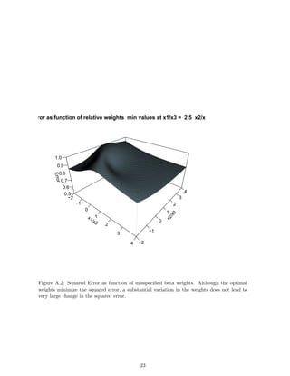
Figure A.2 shows the residual error variance as a function of relative weights of bx1/bx3and
bx2/bx3 for a set of correlated predictors.
R
x1 x2 x3
x1 1.00 0.56 0.48
x2 0.56 1.00 0.42
x3 0.48 0.42 1.00
rxy
x1 x2 x3
y 0.4 0.35 0.3
g(R, rxy)
22

23. x1/x3
−2
−1
0
1
2
3
4
x
2
/
x
3
−2
−1
0
1
2
3
4
E
r
r
o
r
0.5
0.6
0.7
0.8
0.9
1.0
Error as function of relative weights min values at x1/x3 = 2.5 x2/x3 = 1.5
Figure A.2: Squared Error as function of misspecified beta weights. Although the optimal
weights minimize the squared error, a substantial variation in the weights does not lead to
very large change in the squared error.
23

24. x1/x3
−2
−1
0
1
2
3
4
x
2
/
x
3
−2
−1
0
1
2
3
4
E
r
r
o
r
0.5
0.6
0.7
0.8
0.9
1.0
Error as function of relative weights min values at x1/x3 = 1.5 x2/x3 = 1.2
Figure A.3: With orthogonal predictors, the squared error surface is somewhat better defined,
although still large changes in beta weights do not lead to large changes in squared error.
With independent predictors, the response surface is somewhat steeper (Figure A.3), but still
the squared error function does not change vary rapidly as the beta weights change. This
phenomenon has been well discussed by Robyn Dawes and his colleagues.
x1 x2 x3
x1 1 0 0
x2 0 1 0
x3 0 0 1
x1 x2 x3
y 0.4 0.35 0.3
24