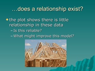
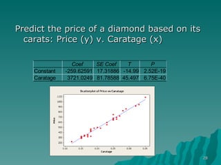
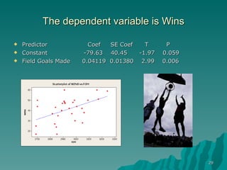
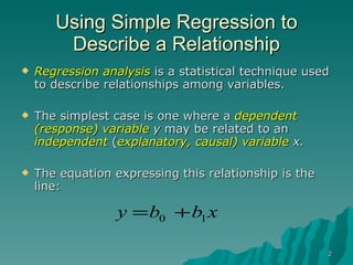
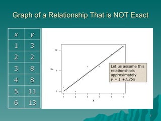
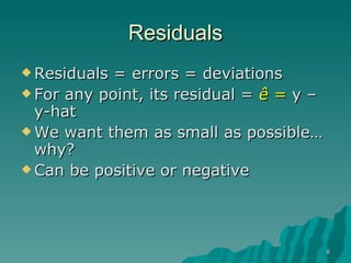
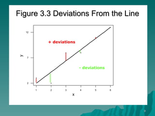
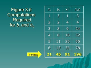
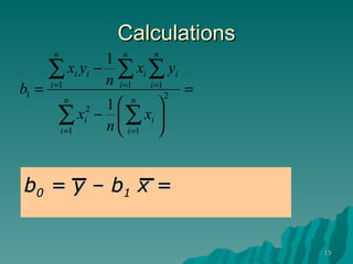
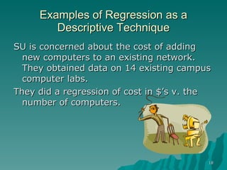
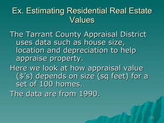
This document discusses using simple linear regression to describe relationships between variables in data. It explains that regression finds the linear equation that best describes how a dependent variable (y) changes with an independent variable (x). The equation is the line that minimizes the sum of the squared residuals (deviations from the observed data points). Examples are given of regression analyses conducted to estimate the cost of computer networks based on number of computers, estimate real estate values based on house size, and forecast housing starts based on mortgage rates.

1. Using Regression to Describe Relationships in Data (Ch 3) Simple Regression ** Multiple Regression

2. Using Simple Regression to Describe a Relationship Regression analysis is a statistical technique used to describe relationships among variables. The simplest case is one where a dependent (response) variable y may be related to an independent ( explanatory, causal) variable x. The equation expressing this relationship is the line:

3. Algebra refresher

4. Graph of An Exact Relationship y = 1 + 2x x y 1 3 2 5 3 7 4 9 5 11 6 13

5. What about this?

6. Error in the Relationship In real life, we usually do not have exact relationships. Figure 3.2 shows a situation where the y and x have a strong tendency to increase together but it is not perfect. ^ A good guess might be y = 1 + 2.5x

7. Graph of a Relationship That is NOT Exact Let us assume this relationshipis approximately y = 1 +1.25x x y 1 3 2 2 3 8 4 8 5 11 6 13

8. Residuals Residuals = errors = deviations For any point, its residual = ê = y – y-hat We want them as small as possible… why? Can be positive or negative

9. Figure 3.3 Deviations From the Line - deviations + deviations

10. Computation Ideas (1) We can search for a line that minimizes the sum of the residuals: While this is a good idea, it can be shown that any line passing through the point ( x, y ) will have this sum = 0.

11. Computation Ideas (2) We can work with absolute values and search for a line that minimizes: Such a procedure—called LAV or least absolute value regression—does exist but usually is found only in specialized software.

12. Computation Ideas (3) By far the most popular approach is to square the residuals and minimize: This procedure is called least squares and is widely available in software. It uses calculus to solve for the b 0 and b 1 terms and gives a unique solution.

13. Least Squares Estimators There are several formula for the b 1 term. If doing it by hand, we might want to use: _ _ The intercept is b 0 = y – b 1 x

14. Figure 3.5 Computations Required for b 1 and b 0 Totals x i y i x i 2 x i y i 1 3 1 3 2 2 4 4 3 8 9 24 4 8 16 32 5 11 25 55 6 13 36 78 21 45 91 196

15. Calculations _ _ b 0 = y – b 1 x =

16. The Unique Minimum The line we obtained was: This is the best (with smallest error) equation. We guessed y = 1 + 2.5x on slide 7

17. We statistical software!

18. Examples of Regression as a Descriptive Technique SU is concerned about the cost of adding new computers to an existing network. They obtained data on 14 existing campus computer labs. They did a regression of cost in $’s v. the number of computers.

19. Pricing a Computer Network ^ y [Cost] = 16594 + 650 [#computers]

20. Interpreting the equation in words… Slope: on average, each additional computer costs $650 . Or – The cost of the project increases by $650 for each additional computer. Intercept: Must meet all of the following conditions: Fixed cost? Did we collect data at x = 0? Does it make practical sense to build a network of 0 computers? Prediction: on average, the cost for adding 10 computers is $23,094 ($16594 + $650 x 10) ^ y [Cost] = 16594 + 650 [#computers]

21. Ex. Estimating Residential Real Estate Values The Tarrant County Appraisal District uses data such as house size, location and depreciation to help appraise property. Here we look at how appraisal value ($’s) depends on size (sq feet) for a set of 100 homes. The data are from 1990.

22. Tarrant County Real Estate ^ y [Value] = -50035 + 72.8 [sq feet]

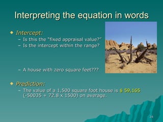
23. Interpreting the equation in words Slope: On average, each additional square foot increases the appraisal value of a house by $72.80. Better -- on average, each additional 100 sq feet raises the appraisal value of a house by $7,280 . Or -- The appraisal value of a house rises by about $7280 for each additional 100 square feet. ^ y [Value] = -50035 + 72.8 [sq feet]

24. Interpreting the equation in words Intercept: Is this the “fixed appraisal value?” Is the intercept within the range? A house with zero square feet??? Prediction: The value of a 1,500 square foot house is $ 59,165 (-50035 + 72.8 x 1500) on average.

25. Ex. Forecasting Housing Starts Here we analyze the relationship between US housing starts and mortgage rates. The rate used is the US average for new home purchases. Annual data from 1963 to 2002 is used.

26. US Housing Starts ^ y [starts] = 1726 - 22.2 [rates]

27. … does a relationship exist? the plot shows there is little relationship in these data Is this reliable? What might improve this model?

28. Predict the price of a diamond based on its carats: Price (y) v. Caratage (x)

29. The dependent variable is Wins Predictor Coef SE Coef T P Constant -79.63 40.45 -1.97 0.059 Field Goals Made 0.04119 0.01380 2.99 0.006

30. Predict # calls by CSR in call center The regression equation is CALLS = 13.7 + 0.744 MONTHS Predictor Coef SE Coef T P Constant 13.671 1.427 9.58 0.000 MONTHS 0.74351 0.06666 11.15 0.000

31. Assignment Study Text 3.1 – 3.2 and lecture notes Study table 3.14 on page 84 We will start HW/Lab 1 together. A short quiz will cover the lab, text, and lecture material Review Text Chapter 2.1-2.2 and PPt Review of Basic Statistics 2.1-2.2 (why? questions on descriptive statistics and plots will be on quiz also!)