Download as PDF, PPTX


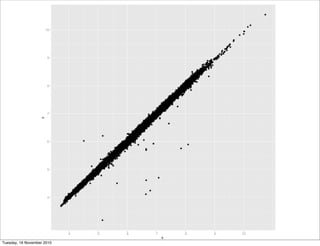
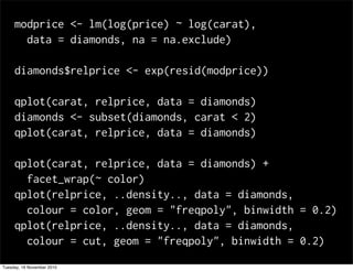
![library(ggplot2)
diamonds$x[diamonds$x == 0] <- NA
diamonds$y[diamonds$y == 0] <- NA
diamonds$y[diamonds$y > 30] <- NA
diamonds$z[diamonds$z == 0] <- NA
diamonds$z[diamonds$z > 30] <- NA
diamonds <- subset(diamonds, carat < 2)
qplot(x, y, data = diamonds)
qplot(x, z, data = diamonds)
Tuesday, 16 November 2010](https://image.slidesharecdn.com/24-modelling-101116153046-phpapp02/85/24-modelling-13-320.jpg)
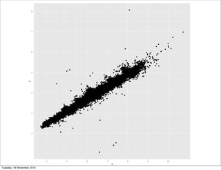
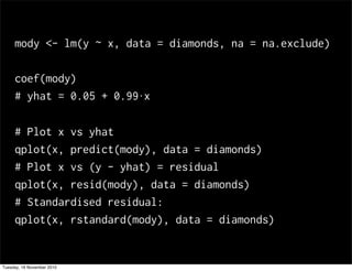
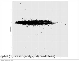
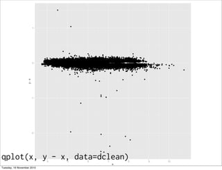
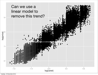
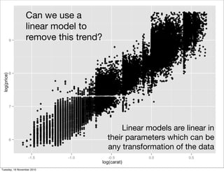
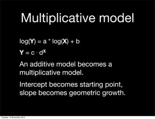
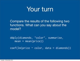
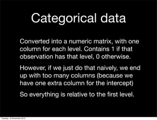
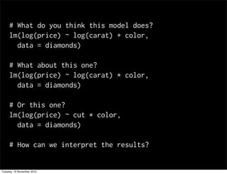
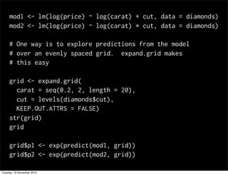

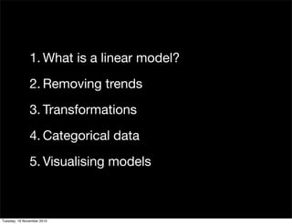
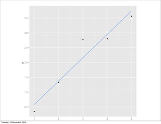
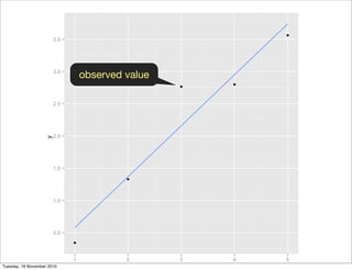
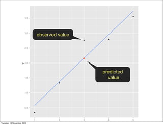
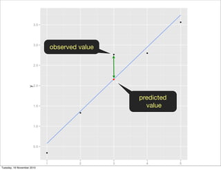
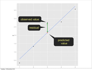
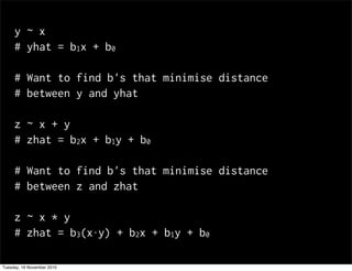
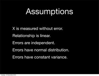
This document summarizes Hadley Wickham's lecture on linear models. It discusses key concepts like what a linear model is, removing trends through transformations, handling categorical data, and visualizing models. Examples using diamonds data demonstrate fitting linear models to predict price from carat and exploring interactions between predictors.


![Introduction to R for Data Science :: Session 6 [Linear Regression in R]](https://cdn.slidesharecdn.com/ss_thumbnails/intrordatasciencesession6eng-160606173046-thumbnail.jpg?width=640&height=640&fit=bounds)


