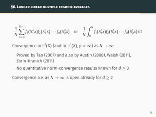
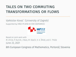
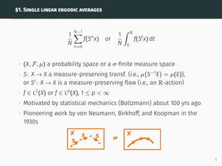
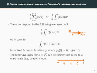
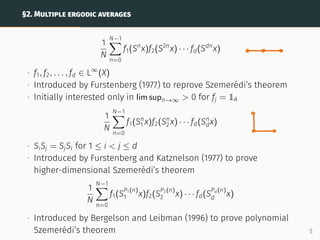
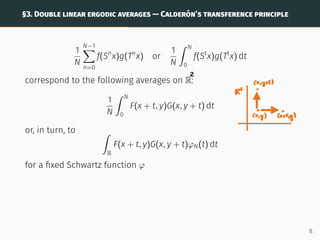
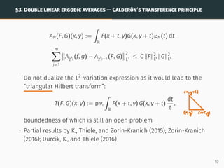
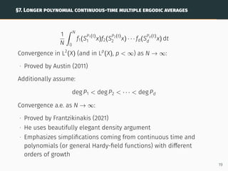
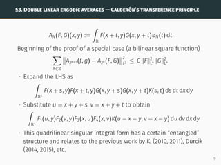
1) The document summarizes recent work on ergodic averages and flows for commuting transformations. It discusses convergence results for single and double linear ergodic averages in L2 and almost everywhere, as well as providing norm estimates to quantify the rate of convergence. 2) It also considers double polynomial ergodic averages and provides proofs for almost everywhere convergence in the continuous-time setting. Open problems remain for the discrete-time case. 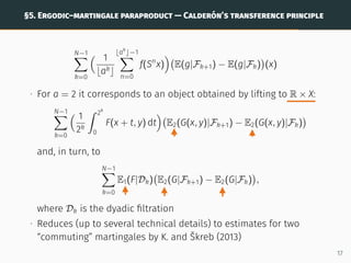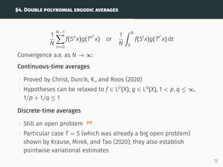3) An ergodic-martingale paraproduct is introduced, motivated by an open question from 1950. Convergence in Lp norm is shown, while almost everywhere convergence remains open.

1. TALES ON TWO COMMUTING
TRANSFORMATIONS OR FLOWS
Vjekoslav Kovač (University of Zagreb)
Supported by HRZZ IP-2018-01-7491 (DEPOMOS)
Based on joint work with
M. Christ, P. Durcik, J. Roos, M. Stipčić, K. A. Škreb, and C. Thiele
June 23, 2021
8th European Congress of Mathematics, Portorož, Slovenia

2. §1. SINGLE LINEAR ERGODIC AVERAGES
1
N
N−1
X
n=0
f(Sn
x) or
1
N
ˆ N
0
f(St
x) dt
∙ (X, F, µ) a probability space or a σ-finite measure space
∙ S: X → X a measure-preserving transf. (i.e., µ S−1
E
= µ(E)),
or St
: X → X is a measure-preserving flow (i.e., an R-action)
∙ f ∈ L2
(X) or f ∈ Lp
(X), 1 ≤ p ∞
∙ Motivated by statistical mechanics (Boltzmann) about 100 yrs ago
∙ Pioneering work by von Neumann, Birkhoff, and Koopman in the
1930s
1

3. §1. SINGLE LINEAR ERGODIC AVERAGES — NORM CONVERGENCE
1
N
N−1
X
n=0
f(Sn
x) or
1
N
ˆ N
0
f(St
x) dt
L2
convergence as N → ∞:
∙ Proved by von Neumann (1932)
∙ Can we quantify the L2
convergence by controlling the number of
jumps in the norm?
Norm-variation estimate [Jones, Ostrovskii, and Rosenblatt (1996)]
sup
N0N1···Nm
m
X
j=1
ANj
f − ANj−1
f
2
L2
1/2
≤ C kfkL2
∙ They work on T ≡ S1
and then use the spectral theorem for the
unitary operator f 7→ f ◦ S (the Koopman operator)
Consequence
ANf make O(ε−2
kfk2
L2 ) jumps of size ≥ ε in the L2
norm
2

4. §1. SINGLE LINEAR ERGODIC AVERAGES — A.E. CONVERGENCE
1
N
N−1
X
n=0
f(Sn
x) or
1
N
ˆ N
0
f(St
x) dt
Pointwise a.e. convergence as N → ∞:
∙ Proved by Birkhoff (1931)
∙ Can we quantify the a.e. convergence by controlling the number of
jumps along almost all trajectories?
Pointwise variational estimate [Bourgain (1988), Jones, Kaufman,
Rosenblatt, and Wierdl (1998)]
sup
N0N1···Nm
m
X
j=1
|ANj
f − ANj−1
f|ϱ
1/ϱ
Lp
≤ Cp,ϱ kfkLp
for 2 ϱ ∞, 1 p ∞
∙ Bourgain actually studied more general, discrete single polynomial
averages
3

5. §1. SINGLE LINEAR ERGODIC AVERAGES — CALDERÓN’S TRANSFERENCE PRINCIPLE
1
N
N−1
X
n=0
f(Sn
x) or
1
N
ˆ N
0
f(St
x) dt
∙ These correspond to the following averages on R:
1
N
ˆ N
0
F(x + t) dt
or, in turn, to ˆ
R
F(x + t)φN(t) dt
for a fixed Schwartz function φ, where φN(t) := N−1
φ(N−1
t)
∙ The latter averages (for N = 2k
) can be further compared to a
martingale (e.g., dyadic) model
4

6. §2. MULTIPLE ERGODIC AVERAGES
1
N
N−1
X
n=0
f1(Sn
x)f2(S2n
x) · · · fd(Sdn
x)
∙ f1, f2, . . . , fd ∈ L∞
(X)
∙ Introduced by Furstenberg (1977) to reprove Szemerédi’s theorem
∙ Initially interested only in lim supn→∞ 0 for fj = 1A
1
N
N−1
X
n=0
f1(Sn
1 x)f2(Sn
2 x) · · · fd(Sn
dx)
∙ SiSj = SjSi for 1 ≤ i j ≤ d
∙ Introduced by Furstenberg and Katznelson (1977) to prove
higher-dimensional Szemerédi’s theorem
1
N
N−1
X
n=0
f1(S
P1(n)
1 x)f2(S
P2(n)
2 x) · · · fd(S
Pd(n)
d x)
∙ Introduced by Bergelson and Leibman (1996) to prove polynomial
Szemerédi’s theorem 5

7. §3. DOUBLE LINEAR ERGODIC AVERAGES
1
N
N−1
X
n=0
f(Sn
x)g(Tn
x) or
1
N
ˆ N
0
f(St
x)g(Tt
x) dt
The setting:
∙ ST = TS or Ss
Tt
= Tt
Ss
∙ f, g ∈ L∞
(X)
Convergence in L2
(X) (and in Lp
(X), p ∞) as N → ∞:
∙ Proved by Conze and Lesigne (1984)
Convergence a.e. as N → ∞:
∙ It is an old open problem! (Calderón? Furstenberg?)
∙ Particular case T = S−1
shown by Bourgain (1990), with a pointwise
variational estimate by Do, Oberlin, and Palsson (2015)
∙ “Additionally averaged” aver. handled by Donoso and Sun (2016)
6

8. §3. DOUBLE LINEAR ERGODIC AVERAGES
1
N
N−1
X
n=0
f(Sn
x)g(Tn
x) or
1
N
ˆ N
0
f(St
x)g(Tt
x) dt
∙ Can we quantify L2
convergence in the sense of controlling the
number of jumps?
∙ This can also be considered as partial progress towards a.e.
convergence (Bourgain’s metric entropy bounds)
∙ A question by Avigad and Rute (2012); also by Bourgain?
Norm-variation estimate [Durcik, K., Škreb, and Thiele (2016)]
sup
N0N1···Nm
m
X
j=1
ANj
(f, g) − ANj−1
(f, g)
2
L2
1/2
≤ C kfkL4 kgkL4
7

9. §3. DOUBLE LINEAR ERGODIC AVERAGES — CALDERÓN’S TRANSFERENCE PRINCIPLE
1
N
N−1
X
n=0
f(Sn
x)g(Tn
x) or
1
N
ˆ N
0
f(St
x)g(Tt
x) dt
correspond to the following averages on R:
1
N
ˆ N
0
F(x + t, y)G(x, y + t) dt
or, in turn, to ˆ
R
F(x + t, y)G(x, y + t)φN(t) dt
for a fixed Schwartz function φ
8

10. §3. DOUBLE LINEAR ERGODIC AVERAGES — CALDERÓN’S TRANSFERENCE PRINCIPLE
AN(F, G)(x, y) :=
ˆ
R
F(x + t, y)G(x, y + t)φN(t) dt
Beginning of the proof of a special case (a bilinear square function)
X
k∈Z
A2k+1 (f, g) − A2k (F, G)
2
L2 ≤ C kFk2
L4 kGk2
L4
∙ Expand the LHS as
ˆ
R4
F(x + s, y)F(x + t, y)G(x, y + s)G(x, y + t)K(s, t) ds dt dx dy
∙ Substitute u = x + y + s, v = x + y + t to obtain
ˆ
R4
F1(u, y)F2(v, y)F3(x, u)F4(x, v)K(u − x − y, v − x − y) du dv dx dy
∙ This quadrilinear singular integral form has a certain “entangled”
structure and relates to the previous work by K. (2010, 2011), Durcik
(2014, 2015), etc.
9

11. §3. DOUBLE LINEAR ERGODIC AVERAGES — CALDERÓN’S TRANSFERENCE PRINCIPLE
AN(F, G)(x, y) :=
ˆ
R
F(x + t, y)G(x, y + t)φN(t) dt
m
X
j=1
A2
kj (f, g) − A2
kj−1 (F, G)
2
L2 ≤ C kFk2
L4 kGk2
L4
∙ Do not dualize the L2
-variation expression as it would lead to the
“triangular Hilbert transform”:
T(F, G)(x, y) := p.v.
ˆ
R
F(x + t, y) G(x, y + t)
dt
t
,
boundedness of which is still an open problem
∙ Partial results by K., Thiele, and Zorin-Kranich (2015); Zorin-Kranich
(2016); Durcik, K., and Thiele (2016)
10

12. §4. DOUBLE POLYNOMIAL ERGODIC AVERAGES
1
N
N−1
X
n=0
f(Sn
x)g(Tn2
x) or
1
N
ˆ N
0
f(St
x)g(Tt2
x) dt
The setting:
∙ ST = TS or Ss
Tt
= Tt
Ss
∙ f, g ∈ L∞
(X)
Convergence in L2
(X) (and in Lp
(X), p ∞) as N → ∞:
∙ Proved by Bergelson and Leibman (1996), in much higher generality
∙ Continuous-time result is strictly speaking a consequence of
discrete-to-continuous transference by Bergelson, Leibman, and
Moreira (2011)
11

13. §4. DOUBLE POLYNOMIAL ERGODIC AVERAGES
1
N
N−1
X
n=0
f(Sn
x)g(Tn2
x) or
1
N
ˆ N
0
f(St
x)g(Tt2
x) dt
Convergence a.e. as N → ∞:
Continuous-time averages
∙ Proved by Christ, Durcik, K., and Roos (2020)
∙ Hypotheses can be relaxed to f ∈ Lp
(X), g ∈ Lq
(X), 1 p, q ≤ ∞,
1/p + 1/q ≤ 1
Discrete-time averages
∙ Still an open problem
∙ Particular case T = S (which was already a big open problem)
shown by Krause, Mirek, and Tao (2020); they also establish
pointwise variational estimates
12

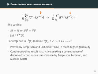
14. §4. DOUBLE POLYNOMIAL CONTINUOUS-TIME ERGODIC AVERAGES
Pointwise convergence result [Christ, Durcik, K., and Roos (2020)]
lim
N→∞
1
N
ˆ N
0
f(St
x)g(Tt2
x) dt exists a.e.
A few ingredients of the proof:
∙ We transfer the estimate
1
N
ˆ N
0
F(x + t + δ, y) − F(x + t, y)
G(x, y + t2
) dt
L1
(x,y)
≤ Cγ,δN−γ
∥F∥L2 ∥G∥L2
for δ 0 and γ = γ(δ) 0 from R2
to the meas.-preserving system
∙ This estimate is, in turn, shown as a consequence of a powerful
“trilinear smoothing estimate” (a “local estimate”) by Christ, Durcik,
and Roos (2020)
∙ We are partly quantitative, partly relying on density arguments
13

15. §5. ERGODIC–MARTINGALE PARAPRODUCT
N−1
X
k=0
1
bakc
⌊ak
⌋−1
X
n=0
f(Sn
x)
E(g|Fk+1) − E(g|Fk)
(x)
∙ A hybrid object that combines ergodic averages and martingales
∙ Motivated by an open-ended question of Kakutani (1950)
∙ S: X → X is measure-preserving
∙ F0 ⊇ F1 ⊇ F2 ⊇ · · · so that E(g|Fn) is a backward (i.e., reversed)
martingale
∙ Commutativity assumption: E(h ◦ S|Fn) = E(h|Fn) ◦ S
∙ 1 a ∞, f ∈ Lp
(X), g ∈ Lq
(X)
14

16. §5. ERGODIC–MARTINGALE PARAPRODUCT
N−1
X
k=0
1
bakc
⌊ak
⌋−1
X
n=0
f(Sn
x)
E(g|Fk+1) − E(g|Fk)
(x)
Convergence in norm as N → ∞:
∙ If 1/p + 1/q = 1/r, p, q ∈ [4/3, 4], r ∈ [1, 4/3], then convergence in
the Lr
norm was shown by K. and Stipčić (2020)
∙ The main part is mere Lp
× Lq
→ Lr
boundedness (nontrivial here)
Convergence pointwise a.e. as N → ∞:
∙ Still an open problem
∙ Could be a nice toy-problem for the famous open problem on
double linear averages w.r.t. two commuting transformations
15

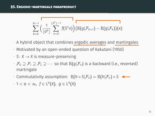
17. §5. ERGODIC–MARTINGALE PARAPRODUCT — BOUNDEDNESS
N−1
X
k=0
1
bakc
⌊ak
⌋−1
X
n=0
f(Sn
x)
E(g|Fk+1) − E(g|Fk)
(x)
Boundedness of the erg.–mart. paraprod. [K. and Stipčić (2020)]
kΠN(f, g)kLr =
N−1
X
k=0
(Akf)(Ek+1g − Ekg)
Lr
≤ Ca,p,q,r kfkLp kgkLq
for 1/p + 1/q = 1/r, p, q ∈ [4/3, 4], r ∈ [1, 4/3]
=⇒ kΠN(f, g) − ΠM(f, g)kLr ≤ Ca,p,q,r kfkLp kENg − EMgkLq
so convergence in Lr
(X) follows
16

18. §5. ERGODIC–MARTINGALE PARAPRODUCT — CALDERÓN’S TRANSFERENCE PRINCIPLE
N−1
X
k=0
1
bakc
⌊ak
⌋−1
X
n=0
f(Sn
x)
E(g|Fk+1) − E(g|Fk)
(x)
∙ For a = 2 it corresponds to an object obtained by lifting to R × X:
N−1
X
k=0
1
2k
ˆ 2k
0
F(x + t, y) dt
E2(G(x, y)|Fk+1) − E2(G(x, y)|Fk)
and, in turn, to
N−1
X
k=0
E1(F|Dk) E2(G|Fk+1) − E2(G|Fk)
,
where Dk is the dyadic filtration
∙ Reduces (up to several technical details) to estimates for two
“commuting” martingales by K. and Škreb (2013)
17

19. §6. LONGER LINEAR MULTIPLE ERGODIC AVERAGES
1
N
N−1
X
n=0
f1(Sn
1 x)f2(Sn
2 x) · · · fd(Sn
dx) or
1
N
ˆ N
0
f1(St
1x)f2(St
2x) · · · fd(St
dx) dt
Convergence in L2
(X) (and in Lp
(X), p ∞) as N → ∞:
∙ Proved by Tao (2007) and also by Austin (2008), Walsh (2011),
Zorin-Kranich (2011)
∙ No quantitative norm-convergence results known for d ≥ 3
Convergence a.e. as N → ∞ is open already for d ≥ 2
18

20. §7. LONGER POLYNOMIAL CONTINUOUS-TIME MULTIPLE ERGODIC AVERAGES
1
N
ˆ N
0
f1(S
P1(t)
1 x)f2(S
P2(t)
2 x) · · · fd(S
Pd(t)
d x) dt
Convergence in L2
(X) (and in Lp
(X), p ∞) as N → ∞:
∙ Proved by Austin (2011)
Additionally assume:
deg P1 deg P2 · · · deg Pd
Convergence a.e. as N → ∞:
∙ Proved by Frantzikinakis (2021)
∙ He uses beautifully elegant density argument
∙ Emphasizes simplifications coming from continuous time and
polynomials (or general Hardy-field functions) with different
orders of growth
19

21. THANK YOU FOR YOUR ATTENTION!
20