Downloaded 42 times


![times <- ddply(bnames, "name", summarise,
boys = sum(prop[sex == "boy"]),
boys_n = sum(sex == "boy"),
girls = sum(prop[sex == "girl"]),
girls_n = sum(sex == "girl"),
.progress = "text"
)
Useful for slow operations
# But this is rather painful
Tuesday, 5 October 2010](https://image.slidesharecdn.com/13-case-study-101005154158-phpapp01/85/13-case-study-16-320.jpg)


![rng <- ddply(selected, "name", summarise,
diff = diff(range(lratio, na.rm = T)),
mean = mean(lratio, na.rm = T)
)
qplot(diff, abs(mean), data = rng)
qplot(diff, abs(mean), data = rng, geom = "text",
label = name)
rng$dual <- abs(rng$mean) < 2
arrange(rng, mean, dual)
selected <- join(selected, rng[c("name", "dual")]
Tuesday, 5 October 2010](https://image.slidesharecdn.com/13-case-study-101005154158-phpapp01/85/13-case-study-24-320.jpg)


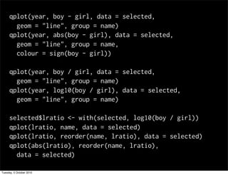
This document discusses a case study analyzing gender trends in baby names: 1. It focuses on analyzing a smaller subset of the most popular names over time. 2. The document computes summary statistics like the proportion of babies given each name that were boys or girls and the number of years each name was in the top 1000 for boys and girls. 3. Names are classified as either having dual or separate gender usage over time based on the ratio of boy to girl name assignments each year.


