Downloaded 95 times


![5
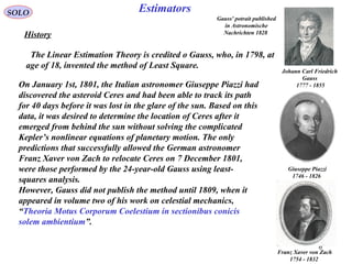
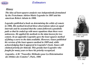
Estimators
v
( )vxh , z
x
SOLO
Desirable Properties of Estimators.
( ){ } ( ){ } ( )kxZkxEkxE k
== ,ˆˆ
Unbiased Estimator1
Consistent or Convergent Estimator2
( ) ( )[ ] ( ) ( )[ ]{ } 00ˆˆProblim =>>−−
∞→
εkxkxkxkx
T
k
( ) ( )[ ] ( ) ( )[ ]{ } ( ) ( )[ ] ( ) ( )[ ]{ } KkforkxkxkxkxEkxkxkxkxE
TT
>−−≤−− γγ ˆˆˆˆ
Efficient or Assymptotic Efficient Estimator if for All Unbiased Estimators3 ( )( )kxγγ ˆ
Sufficient Estimator if it contains all the information in the set of observed values
regarding the parameter to be observed.
4 k
Z
( )kx
Table of Content](https://image.slidesharecdn.com/2-estimators-150110062422-conversion-gate02/85/2-estimators-5-320.jpg)


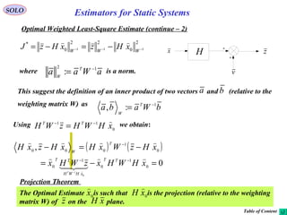
 ( ) ( ) 02/ 0
1
00
22
0
<−−−=−∂∂− −
xxHWHxxxxxJxx TTT
or the matrix HT
W-1
H is positive definite.
W is a hermitian (WH
= W, H stands for complex conjugate and matrix transpose),
positive definite weighting matrix.](https://image.slidesharecdn.com/2-estimators-150110062422-conversion-gate02/85/2-estimators-13-320.jpg)
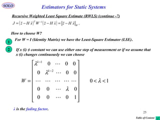
![19
SOLO
Recursive Weighted Least Square Estimate (RWLS) (continue -1)
( ) ( ) 1
0
1
00
:
−−
=− HWHP
T
( ) ( ) 0
1
00
zWHPx
T −
−=−
( ) ( ) [ ] [ ]
( ) ( )zWHzWHHWHHWH
z
z
W
W
HH
H
H
W
W
HHzWHHWHx
TTTT
TTTTTT
1
0
1
00
11
0
1
00
0
1
1
0
0
1
0
1
1
0
01
1
111
1
11
0
0
0
0
−−−−−
−
−
−
−
−
−−
++=
==+
Define ( ) ( ) HWHPHWHHWHP TTT 111
0
1
00
1
: −−−−−
+−=+=+
( ) ( )[ ] ( ) ( ) ( )[ ] ( )−+−−−−=+−=+
−−−−
PHWHPHHPPHWHPP TT
LemmaMatrixInverse
T 1111
( ) ( )[ ] ( )[ ] ( ) 111111 −−−−−−
+=+−≡+−− WHPWHHWHPWHPHHP TTTTT
( ) ( ) ( ) ( )[ ] ( ) ( ) ( ) ( )−+−−=−+−−−−=+ −−
PHWHPPPHWHPHHPPP TTT 11
( ) ( )( )
( ) ( ) ( )[ ] ( ){ } ( ) zWHPzWHPHWHPHHPP
zWHzWHPx
TTTT
TT
1
0
1
00
1
1
0
1
00
−−−
−−
++−+−−−−=
++=+
Estimators for Static Systems](https://image.slidesharecdn.com/2-estimators-150110062422-conversion-gate02/85/2-estimators-18-320.jpg)
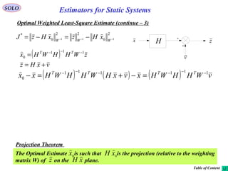
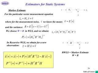
![20
v
H zx
SOLO
Recursive Weighted Least Square Estimate (RWLS) (continue -2)
( ) ( )( )
( ) ( ) ( )[ ] ( ){ } ( )
( )
( )
( ) ( )[ ]
( )
( )
( )
( )
( ) ( ) ( ) ( ) zWHPxHWHPx
zWHPzWHPHWHPHHPzWHP
zWHPzWHPHWHPHHPP
zWHzWHPx
TT
T
x
T
WHP
TT
x
T
TTTT
TT
T
11
1
0
1
00
1
0
1
00
1
0
1
00
1
1
0
1
00
1
−−
−
−
−
+
−
−
−
−−−
−−
++−+−−=
++−+−−−−=
++−+−−−−=
++=+
−
( ) ( ) 0
1
00
zWHPx
T −
−=−
( ) ( ) HWHPP T 111 −−−
+−=+
( ) ( ) ( ) ( )( )−−++−=+ −
xHzWHPxx T 1
Recursive Weighted Least Square Estimate
(RWLS)
z
( )−x
( )+x
Delay
( ) HWHP T 11 −−
=+
H
( ) 1−
+ WHP T
Estimator
Estimators for Static Systems](https://image.slidesharecdn.com/2-estimators-150110062422-conversion-gate02/85/2-estimators-19-320.jpg)
![21
( ) ( )
( ) ( )[ ]
( ) ( ) ( ) ( )xHzWxHzxHzWxHz
xHz
xHz
W
W
xHzxHz
xHz
xHz
W
W
xHz
xHz
xHzWxHzJ
TT
TT
T
T
−−+−−=
−
−
−−=
−
−
−
−
=−−=
−−
−
−
−
−
1
00
1
000
00
1
1
0
00
00
1
000
11
1
1111
0
0
0
0
( ) 0
1
00
1
: HWHP
T −−
=−
SOLO
Recursive Weighted Least Square Estimate (RWLS) (continue -3)
Second Way
We want to prove that
where ( ) ( ) 0
1
00
: zWHPx
T −
−=−
( ) ( ) ( )[ ] ( ) ( )[ ]−−−−−=−− −−
xxPxxxHzWxHz
TT 1
00
1
000
Therefore
( )[ ] ( ) ( )[ ] ( ) ( ) ( ) ( ) 11
11
1 −− −+−−=−−+−−−−−= −
−−
WP
TT
xHzxxxHzWxHzxxPxxJ
Estimators for Static Systems](https://image.slidesharecdn.com/2-estimators-150110062422-conversion-gate02/85/2-estimators-20-320.jpg)
![22
( ) 0
1
00
1
: HWHP
T −−
=−
SOLO
Recursive Weighted Least Square Estimate (RWLS) (continue -4)
Second Way (continue – 1)
We want to prove that
Define
( ) ( ) 0
1
00: zWHPx
T −
−=−
( ) ( )−=−
−
PHWzx
TT
0
1
00
( ) ( )−−= −−
xPzWH
T 1
0
1
00
( ) ( )−−= −− 1
0
1
00 PxHWz TT
( ) ( ) ( )[ ] ( ) ( )[ ]−−−−−=−− −−
xxPxxxHzWxHz
TT 1
00
1
000
( ) ( )
xHWHxzWHxxHWzzWz
xHzWxHz
TTTTTT
T
0
1
000
1
000
1
000
1
00
00
1
000
−−−−
−
+−−=
−−
( )[ ] ( ) ( )[ ]
( ) ( ) ( ) ( ) ( ) ( ) ( ) ( )−−−+−−−−−−−=
−−−−−
−−−−
−
xPxxPxxPxxPx
xxPxx
TTTT
T
1111
1
( ) ( ) xPxxHWz TT
−−= −− 1
0
1
00
( ) ( )−−= −−
xPxzWx TTT 1
0
1
00
R
( ) xHWHxxPx
TTT
0
1
00
1 −−
=−
Estimators for Static Systems](https://image.slidesharecdn.com/2-estimators-150110062422-conversion-gate02/85/2-estimators-21-320.jpg)
![23
( ) 0
1
00
1
: HWHP
T −−
=− ( ) ( ) 0
1
00
: zWHPx
T −
−=−
SOLO
Recursive Weighted Least Square Estimate (RWLS) (continue -5)
Second Way (continue – 2)
We want to prove that
Define
( ) ( ) ( )[ ] ( ) ( )[ ]−−−−−=−− −−
xxPxxxHzWxHz
TT 1
00
1
00
( ) ( )
xHWHxzWHxxHWzzWz
xHzWxHz
TTTTTT
T
0
1
000
1
000
1
000
1
00
00
1
000
−−−−
−
+−−=
−−
( )[ ] ( ) ( )[ ]
( ) ( ) ( ) ( ) ( ) ( ) ( ) ( )−−−+−−−−−−−=
−−−−−
−−−−
−
xPxxPxxPxxPx
xxPxx
TTTT
T
1111
1
( ) ( ) ( ) ( ) 0
1
00
1
0
1
00
1
zWHPHWzxPx
TTT −−−−
−=−−−
Use the identity: ( )
1
00
1
0
1
00
1
0
1
000
1
0
1
0
1
−
−−−−−−
+≡+−
TTT
HIHWWHIHWHHWW
ε
ε
( ) 0lim
1
lim
1
lim
1
00
0
1
00
0
1
00
1
0
0
1
0 ==
=
+−
−
→
−
→
−
−
→
− TTT
HHHHHIHWW ε
εε εεε
( ) ( ) 1
00
1
0
1
0
1
00
1
0
1
000
1
0
1
0
−−−−−−−−
−== WHPHWWHHWHHWW
TTT
( ) ( ) ( ) ( ) 0
1
000
1
00
1
0
1
00
1
zWzzWHPHWzxPx
TTTT −−−−−
=−=−−−
q.e.d.
Estimators for Static Systems](https://image.slidesharecdn.com/2-estimators-150110062422-conversion-gate02/85/2-estimators-22-320.jpg)
![24
( )[ ] ( ) ( )[ ] ( ) ( )xHzWxHzxxPxxJ
TT
−−+−−−−−= −− 11
1
SOLO
Recursive Weighted Least Square Estimate (RWLS) (continue -6)
Second Way (continue – 5)
x
Choose that minimizes the scalar cost function
Solution
( ) ( )[ ] ( ) 022 *1*11
=−−−−−=
∂
∂ −−
xHzWHxxP
x
J T
T
Define: ( ) ( ) HWHPP T 111
: −−−
+−=+
Then:
( ) ( )[ ] ( ) ( ) ( ) ( )[ ]−−+−+=+−−+=+ −−−−−−
xHzWHxPzWHxHWHPxP TTT 11111*1
( )[ ] ( ) ( ) zWHxPxHWHP TT 11*11 −−−−
+−−=+−
( ) ( ) ( ) ( )[ ]−−++−=+= −
xHzWHPxxx T 1*
( )[ ] ( )+=+−=
∂
∂ −−− 111
2
1
2
22 PHWHP
x
J T
T
If P-1
(+) is a positive definite matrix then is a minimum solution.*
x
Estimators for Static Systems](https://image.slidesharecdn.com/2-estimators-150110062422-conversion-gate02/85/2-estimators-23-320.jpg)
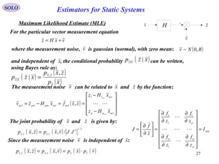
![28
SOLO
Maximum Likelihood Estimate (continue – 1)
v
H zx
( ) ( ) ( ) ( )vpxpvxpzxp vxvxzx ⋅== ,, ,,
x
v
( )vxp vx
,,
( ) ( )
( )
( ) ( )
−−−=
−=
−
xHzRxHz
R
xHzpxzp
T
p
vxz
1
2/12/
|
2
1
exp
2
1
|
π
( ) ( ) ( )[ ] ( )RWWLSxHzRxHzxzp
T
x
xz
x
⇒−−⇔ −1
| min|max
( ) ( )[ ] ( ) 02 11
=−−=−−
∂
∂ −−
xHzRHxHzRxHz
x
TT
0*11
=− −−
xHRHzRH TT
( ) zRHHRHxx TT 111
*: −−−
==
( ) ( )[ ] HRHxHzRxHz
x
TT 11
2
2
2 −−
=−−
∂
∂ this is a positive definite matrix, therefore
the solution minimizes
and maximizes
( ) ( )[ ]xHzRxHz
T
−− −1
( )xzp xz ||
( ) ( )
( )
( )
( )
−=== −
vRv
R
vp
xp
zxp
xzp T
pv
x
zx
xz
1
2/12/
/
|
2
1
exp
2
1,
|
π
Gaussian (normal), with zero mean
( ) ( )xzpxzL xz |:, |=
is called the Likelihood Function and is a measure
of how likely is the parameter given the observation .x z
Estimators for Static Systems](https://image.slidesharecdn.com/2-estimators-150110062422-conversion-gate02/85/2-estimators-27-320.jpg)
![30
SOLO
Bayesian Maximum Likelihood Estimate (Maximum Aposterior – MAP Estimate)
v
H zx
vxHz +=
Consider a gaussian vector , where ,
measurement, , where the Gaussian noise
is independent of and .( )Rv ,0~ N
v
x ( ) ( )[ ]−− Pxx ,~
N
x
( )
( ) ( )
( )( ) ( ) ( )( )
−−−−−−
−
= −
xxPxx
P
xp
T
nx
1
2/12/
2
1
exp
2
1
π
( ) ( )
( )
( ) ( )
−−−=−= −
xHzRxHz
R
xHzpxzp
T
pvxz
1
2/12/|
2
1
exp
2
1
|
π
( ) ( ) ( ) ( )∫∫
+∞
∞−
+∞
∞−
== xdxpxzpxdzxpzp xxzzxz |, |,
is Gaussian with( )zpz ( ) ( ) ( ) ( ) ( )−=+=+= xHvExEHvxHEzE
0
( ) ( )[ ] ( )[ ]{ } ( )[ ] ( )[ ]{ }
( )( )[ ] ( )( )[ ]{ } ( )[ ] ( )[ ]{ }
( )[ ]{ } ( )[ ]{ } { } ( ) RHPHvvEHxxvEvxxEH
HxxxxEHvxxHvxxHE
xHvxHxHvxHEzEzzEzEz
TTTTT
TTT
TT
+−=+−−−−−−
−−−−=+−−+−−=
−−+−−+=−−=
00
cov
( )
( ) ( )
( )[ ] ( )[ ] ( )[ ]
−−+−−−−
+−
=
−
xHzRHPHxHz
RHPH
zp TT
Tpz
ˆˆ
2
1
exp
2
1 1
2/12/
π
Estimators for Static Systems](https://image.slidesharecdn.com/2-estimators-150110062422-conversion-gate02/85/2-estimators-29-320.jpg)
![31
SOLO
Bayesian Maximum Likelihood Estimate (Maximum Aposterior Estimate) (continue – 1)
v
H zx
vxHz +=
Consider a Gaussian vector , where ,
measurement, , where the Gaussian noise
is independent of and .( )Rvv ,0;~ N
v
x ( ) ( )[ ]−− Pxxx ,;~
N
x
( )
( ) ( )
( )( ) ( ) ( )( )
−−−−−−
−
= −
xxPxx
P
xp
T
nx
1
2/12/
2
1
exp
2
1
π
( ) ( )
( )
( ) ( )
−−−=−= −
xHzRxHz
R
xHzpxzp
T
pvxz
1
2/12/|
2
1
exp
2
1
|
π
( )
( ) ( )
( )[ ] ( )[ ] ( )[ ]
−−+−−−−
+−
=
−
xHzRHPHxHz
RHPH
zp TT
Tpz
ˆˆ
2
1
exp
2
1 1
2/12/
π
( )
( ) ( )
( )
( )
( )
( )
( ) ( ) ( )( ) ( ) ( )( ) ( )[ ] ( )[ ] ( )[ ]
−−+−−−+−−−−−−−−−⋅
+−
−
==
−−−
xHzRHPHxHzxxPxxxHzRxHz
RHPH
RPzp
xpxzp
zxp
TTTT
T
nz
xxz
zx
ˆˆ
2
1
2
1
2
1
exp
2
1|
|
111
2/1
2/12/1
2/
|
|
π
from which
Estimators for Static Systems](https://image.slidesharecdn.com/2-estimators-150110062422-conversion-gate02/85/2-estimators-30-320.jpg)
![32
SOLO
Bayesian Maximum Likelihood Estimate (Maximum Aposterior Estimate) (continue – 2)
( ) ( ) ( )( ) ( ) ( )( ) ( )( ) ( )[ ] ( )( )−−+−−−−−−−−−+−−
−−−
xHzRHPHxHzxxPxxxHzRxHz TTTT 111
( ) ( )( )[ ] ( ) ( )( )[ ] ( )( ) ( ) ( )( )
( )( ) ( )[ ] ( )( ) ( )( ) ( )[ ]{ } ( )( )
( )( ) ( )( ) ( )( ) ( )( ) ( )( ) ( )[ ] ( )( )−−+−−−+−−−−−−−−−−
−−+−−−−=−−+−−−−
−−−−−+−−−−−−−−−−=
−−−−
−−−
−−
xxHRHPxxxxHRxHzxHzRHxx
xHzRHPHRxHzxHzRHPHxHz
xxPxxxxHxHzRxxHxHz
TTTTT
TTTT
TT
1111
111
11
( )( ) ( )( ) ( )( ) ( ) ( )( ) ( )( ) ( )[ ] ( )( )−−+−−−−−−−−−+−−−−
−−−
xHzRHPHxHzxxPxxxHzRxHz TTTT 111
( )[ ] ( )[ ] 11111111 −−−−−−−−
−++/−/=+−− RHPHRHHRRRRHPHR TTT
we have
then
Define: ( ) ( )[ ] 111
:
−−−
+−=+ HRHPP T
( )( ) ( ) ( )[ ] ( ) ( )( )
( )( ) ( ) ( )[ ] ( )( ) ( )( ) ( ) ( )[ ] ( )( )
( )( ) ( )[ ] ( )( )−−+−−−+
−−++−−−−−++−−−
−−+++−−=
−−
−−−−
−−−
xxHRHPxx
xxPPHRxHzxHzRHPPxx
xHzRHPPPHRxHz
TT
TTT
TT
11
1111
111
( ) ( ) ( )( )[ ] ( ) ( ) ( ) ( )( )[ ]−−++−−+−−++−−= −−−
xHzRHPxxPxHzRHPxx TTT 111
( )
( ) ( )
( ) ( ) ( )( )[ ] ( ) ( ) ( ) ( )( )[ ]
−−+−−−+−−+−−−−⋅
+
= −−−
xHzRHPxxPxHzRHPxx
P
zxp TTT
nzx
111
2/12/|
2
1
exp
2
1
|
π
Estimators for Static Systems](https://image.slidesharecdn.com/2-estimators-150110062422-conversion-gate02/85/2-estimators-31-320.jpg)
![33
SOLO
Bayesian Maximum Likelihood Estimate (Maximum Aposterior Estimate) (continue – 3)
then
where: ( ) ( )[ ] 111
:
−−−
+−=+ HRHPP T
( )
( ) ( )
( ) ( ) ( )[ ] ( ) ( ) ( ) ( )[ ]
−+−−−+−+−−−−⋅
+
= −−−
xHzRHPxxPxHzRHPxx
P
zxp TTT
nzx
111
2/12/|
2
1
exp
2
1
|
π
( )zxp zx
x
|max | ( ) ( ) ( ) ( )( )−−++−==+ −
xHzRHPxxx T 1*
:
Table of Content
Estimators for Static Systems](https://image.slidesharecdn.com/2-estimators-150110062422-conversion-gate02/85/2-estimators-32-320.jpg)
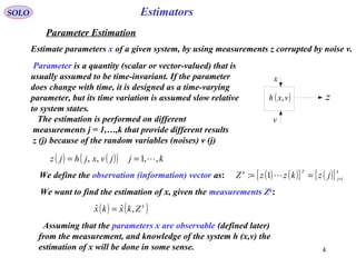
 [ ]( ){ } { } { } { }TTT
x xExExxExExxExE
−=−−=
2
σ - estimated variance matrix
For a good estimator we want
{ } xxE =
- unbiased estimator vector
{ } { } { }TT
x xExExxE
−=
2
σ - minimum estimation variance
( ) ( ){ }Tk
kzzZ 1:= - the observation matrix after k observations
( ) ( ) ( ){ }xkzzLxZL k
,,,1, = - the Likelihood or the joint density function of Zk
We have:
( )T
pzzzz ,,, 21 = ( )T
n
xxxx ,,, 21
= ( )T
pvvvv ,,, 21 =
The estimation of , using the measurements
of a system corrupted by noise is a random variable with
xˆ x z
v
( ) ( ) ( ) ( )∫== dvvpxvZpxZpxZL v
k
vz
k
xz
k
;||, ||
( ) ( )[ ]{ } ( ) ( )[ ] ( ) ( )[ ] ( ) ( )
[ ] [ ] ( )xbxZdxZLZx
kzdzdxkzzLkzzxkzzxE
kkk
+==
=
∫
∫
,
1,,,1,,1,,1
- estimator bias( )xb
therefore:](https://image.slidesharecdn.com/2-estimators-150110062422-conversion-gate02/85/2-estimators-33-320.jpg)
![35
Estimators
v
( )vxh ,
z
x
Estimator
x
SOLO
The Cramér-Rao Lower Bound on the Variance of the Estimator (continue – 1)
[ ]{ } [ ] [ ] ( )xbxZdxZLZxZxE kkkk
+== ∫ ,
We have:
[ ]{ } [ ] [ ] ( )
x
xb
Zd
x
xZL
Zx
x
ZxE k
k
k
k
∂
∂
+=
∂
∂
=
∂
∂
∫ 1
,
Since L [Zk
,x] is a joint density function, we have:
[ ] 1, =∫
kk
ZdxZL
[ ] [ ] [ ] [ ]0
,,
0
,
=
∂
∂
=
∂
∂
→=
∂
∂
∫∫∫
k
k
k
k
k
k
Zd
x
xZL
xZd
x
xZL
xZd
x
xZL
[ ]( ) [ ] ( )
x
xb
Zd
x
xZL
xZx k
k
k
∂
∂
+=
∂
∂
−∫ 1
,
Using the fact that: [ ] [ ] [ ]
x
xZL
xZL
x
xZL k
k
k
∂
∂
=
∂
∂ ,ln
,
,
[ ]( ) [ ] [ ] ( )
x
xb
Zd
x
xZL
xZLxZx k
k
kk
∂
∂
+=
∂
∂
−∫ 1
,ln
,
](https://image.slidesharecdn.com/2-estimators-150110062422-conversion-gate02/85/2-estimators-34-320.jpg)
 [ ] [ ] ( )
x
xb
Zd
x
xZL
xZLxZx k
k
kk
∂
∂
+=
∂
∂
−∫ 1
,ln
,
Hermann Amandus
Schwarz
1843 - 1921
Let use Schwarz Inequality:
( ) ( ) ( ) ( )∫∫∫ ≤ dttgdttfdttgtf
22
2
The equality occurs if and only if f (t) = k g (t)
[ ]( ) [ ] [ ] [ ]xZL
x
xZL
gxZLxZxf k
k
kk
,
,ln
:&,:
∂
∂
=−=
choose:
[ ]( ) [ ] [ ]
( ) [ ]( ) [ ]( ) [ ] [ ]
∂
∂
−≤
∂
∂
+=
∂
∂
−
∫∫
∫
k
k
kkkk
k
k
kk
Zd
x
xZL
xZLZdxZLxZx
x
xb
Zd
x
xZL
xZLxZx
2
2
2
2
,ln
,,1
,ln
,
[ ]( ) [ ]
( )
[ ] [ ]
∫
∫
∂
∂
∂
∂
+
≥−
k
k
k
kkk
Zd
x
xZL
xZL
x
xb
ZdxZLxZx 2
2
2
,ln
,
1
,
](https://image.slidesharecdn.com/2-estimators-150110062422-conversion-gate02/85/2-estimators-35-320.jpg)
 [ ]
( )
[ ] [ ]
∫
∫
∂
∂
∂
∂
+
≥−
k
k
k
kkk
Zd
x
xZL
xZL
x
xb
ZdxZLxZx 2
2
2
,ln
,
1
,
This is the Cramér-Rao bound for a biased estimator
Harald Cramér
1893–1985
Cayampudi Radhakrishna
Rao
1920 -
[ ]{ } ( ) [ ] 1,& =+= ∫
kkk
ZdxZLxbxZxE
[ ]( ) [ ] [ ] [ ]{ } ( )( ) [ ]
[ ] [ ]{ }( ) [ ] ( ) [ ] [ ]{ }( ) [ ]
( ) [ ]
1
2
0
2
22
,
,2,
,,
∫
∫∫
∫∫
+
−+−=
+−=−
kk
kkkkkkkk
kkkkkkk
ZdxZLxb
ZdxZLZxEZxxbZdxZLZxEZx
ZdxZLxbZxEZxZdxZLxZx
[ ] [ ]{ }( ) [ ]
( )
[ ] [ ]
( )xb
Zd
x
xZL
xZL
x
xb
ZdxZLZxEZx
k
k
k
kkkk
x
2
2
2
22
,ln
,
1
, −
∂
∂
∂
∂
+
≥−=
∫
∫
σ](https://image.slidesharecdn.com/2-estimators-150110062422-conversion-gate02/85/2-estimators-36-320.jpg)
![38
EstimatorsSOLO
The Cramér-Rao Lower Bound on the Variance of the Estimator (continue – 4)
[ ] [ ]{ }( ) [ ]
( )
[ ] [ ]
( )xb
Zd
x
xZL
xZL
x
xb
ZdxZLZxEZx
k
k
k
kkkk
x
2
2
2
22
,ln
,
1
, −
∂
∂
∂
∂
+
≥−=
∫
∫
σ
[ ] [ ]
[ ]
[ ]
[ ] [ ] [ ] 0,
,ln
0
,
1,
,
,
,ln
=
∂
∂
→=
∂
∂
→= ∫∫∫
∂
∂
=
∂
∂
kk
kxZL
x
xZL
x
xZL
k
k
kk
ZdxZL
x
xZL
Zd
x
xZL
ZdxZL
k
k
k
[ ] [ ] [ ] [ ] [ ]
[ ]
0,
,ln,ln
,
,ln
,
2
2
=
∂
∂
∂
∂
+
∂
∂
→ ∫∫
∂
∂
∂
∂
k
x
xZL
k
kk
kk
kx
ZdxZL
x
xZL
x
xZL
ZdxZL
x
xZL
k
[ ] [ ] 0
,ln,ln
2
2
2
=
∂
∂
+
∂
∂
→
∂
∂
x
xZL
E
x
xZL
E
kkx
( )
[ ]
( )
( )
[ ]
( )xb
x
xZL
E
x
xb
xb
x
xZL
E
x
xb
k
k
x
2
2
2
2
2
2
2
2
,ln
1
,ln
1
−
∂
∂
∂
∂
+
−=−
∂
∂
∂
∂
+
≥σ](https://image.slidesharecdn.com/2-estimators-150110062422-conversion-gate02/85/2-estimators-37-320.jpg)
 [ ]
( )
[ ]
( )
[ ]
∂
∂
∂
∂
+
−=
∂
∂
∂
∂
+
≥−∫
2
2
2
2
2
2
,ln
1
,ln
1
,
x
xZL
E
x
xb
x
xZL
E
x
xb
ZdxZLxZx kk
kkk
SOLO
The Cramér-Rao Lower Bound on the Variance of the Estimator (continue – 5)
( )
[ ]
( )
( )
[ ]
( )xb
x
xZL
E
x
xb
xb
x
xZL
E
x
xb
k
k
x
2
2
2
2
2
2
2
2
,ln
1
,ln
1
−
∂
∂
∂
∂
+
−=−
∂
∂
∂
∂
+
≥σ
For an unbiased estimator (b (x) = 0), we have:
[ ] [ ]
∂
∂
−=
∂
∂
≥
2
22
2
,ln
1
,ln
1
x
xZL
E
x
xZL
E
k
k
x
σ
http://www.york.ac.uk/depts/maths/histstat/people/cramer.gif](https://image.slidesharecdn.com/2-estimators-150110062422-conversion-gate02/85/2-estimators-38-320.jpg)
 [ ]( ) [ ] [ ]( ) [ ]( ){ }
( ) [ ] [ ] ( )
( ) [ ] ( )
∂
∂
+
∂
∂
∂
∂
+−=
∂
∂
+
∂
∂
∂
∂
∂
∂
+≥
−−=−−
−
−
∫
x
xb
I
x
xZL
E
x
xb
I
x
xb
I
x
xZL
x
xZL
E
x
xb
I
xZxxZxEZdxZLxZxxZx
x
k
T
x
T
kk
T
x
TkkkkTkk
1
2
2
1
,ln
,ln,ln
,
SOLO
The Cramér-Rao Lower Bound on the Variance of the Estimator (continue – 5)
The multivariable form of the Cramér-Rao Lower Bound is:
[ ]( )
[ ]
[ ]
−
−
=−
n
k
n
k
k
xZx
xZx
xZx
11
[ ]( ) [ ]
[ ]
[ ]
∂
∂
∂
∂
=
∂
∂
=∇
n
k
k
k
k
x
x
xZL
x
xZL
x
xZL
xZL
,ln
,ln
,ln
,ln
1
Fisher Information Matrix
[ ] [ ] [ ]
∂
∂
−=
∂
∂
∂
∂
=
x
k
x
T
kk
x
xZL
E
x
xZL
x
xZL
E 2
2
,ln,ln,ln
:J
Fisher, Sir Ronald Aylmer
1890 - 1962](https://image.slidesharecdn.com/2-estimators-150110062422-conversion-gate02/85/2-estimators-39-320.jpg)
 [ ]( ){ } [ ]( ){ }x
k
xx
x
Tk
x
k
x
xZLExZLxZLEx ,ln,ln,ln: ∇∇−=∇∇=J
Table of Content](https://image.slidesharecdn.com/2-estimators-150110062422-conversion-gate02/85/2-estimators-40-320.jpg)
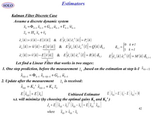
![43
Estimators
kkkkk xxx −= −− 1|1|
ˆ:~
kkkkkkk zKxKx += −1||
ˆ'ˆ
SOLO
Kalman Filter Discrete Case (continue – 1)
Define
kkkkk xxx −= ||
ˆ:~
The Linear Estimator we want is:
Therefore
[ ] [ ] [ ] kkkkkkkkk
z
kkkk
x
kkkkkkk vKxKxIHKKvxHKxxKxx
kkk
++−+=++++−= −−
−
1|
ˆ
1||
~''~'~
1|
Unbiaseness conditions: { } { } 0~~
1|| == −kkkk xExE
gives: { } [ ] { } { } { } 0~''~
00
1|
0
| =++−+= −
kkkkkkkkkkk vEKxEKxEIHKKxE
or: kkk HKIK −='
Therefore the Unbiased Linear Estimator is:
[ ]1|1||
ˆˆˆ −− −+= kkkkkkkkk xHzKxx](https://image.slidesharecdn.com/2-estimators-150110062422-conversion-gate02/85/2-estimators-42-320.jpg)
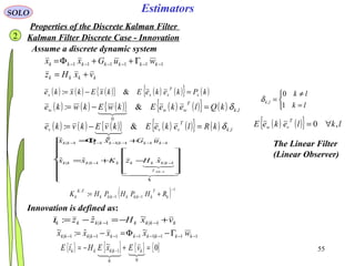
![44
Estimators
+=
Γ++Φ= −−−−−−
kkkk
kkkkkkk
vxHz
wuGxx 111111
SOLO
Kalman Filter Discrete Case (continue – 2)
The discrete dynamic system
The Linear Filter
(Linear Observer)[ ]
−++=
+Φ=
−−−−
−−−−−−
1|111||
111|111|
ˆˆˆ
ˆˆ
kkkkkkkkkkk
kkkkkkk
xHzKuGxx
uGxx
111|111|1|
~ˆ:~
−−−−−−− Γ−Φ=−= kkkkkkkkkk wxxxx
{ } T
kkk
T
kkkk
T
kkkkkk QPxxEP 11111|111|1|1|
~~: −−−−−−−−−− ΓΓ+ΦΦ==
{ } { } { }
{ } { } { } { }
{ } { } { }0~
00
0~~
1111
1
1||
==
==
==
−−−−
−
−
T
kk
T
kk
kk
kkkk
wxEwxE
wEvE
xExE
{ }
[ ] [ ]{ }
{ } { }
{ } { } T
k
T
kkk
T
k
T
kkk
T
k
T
kkk
T
k
T
kkk
T
k
T
k
T
k
T
kkkkk
T
kkkkkk
wwExwE
wxExxE
wxwxE
xxEP
11111
0
111
1
0
1111111
11111111
1|1|1|
~
~~~
~~
~~:
−−−−−−−−
−−−−−−−−
−−−−−−−−
−−−
ΓΓ+ΦΓ−
ΓΦ−ΦΦ=
Γ−ΦΓ−Φ=
=
{ } { } { } 1111
0
1|111|
1
~~
−−−−−−−− Γ−=Γ−Φ=
−
kk
M
T
kkkkkkk
T
kkk MvwEvxEvxE
k
](https://image.slidesharecdn.com/2-estimators-150110062422-conversion-gate02/85/2-estimators-43-320.jpg)
![45
EstimatorsSOLO
Kalman Filter Discrete Case (continue – 3)
{ }kkkkkkkkkkkk vxHKxxxx −−=−= −− 1|1|||
~~ˆ:~
{ } ( )[ ] ( )[ ]{ }T
k
T
k
T
k
T
kk
T
kkkkkkkkk
T
kkkkkk KvHxxvxHKxExxEP −−−−== −−−− 1|1|1|1||||
~~~~~~:
{ } 111|
~
−−− Γ−= kk
T
kkk MvxE
( ) { }( ) { }[ ]
{ }( ) { }[ ]T
k
T
kkk
T
k
T
k
T
kkkk
T
k
T
kkk
T
k
T
k
T
kkkkkk
KxvEKHIxvEK
KvxEKHIxxEHKI
1|1|
1|1|1|
~~
~~~
−−
−−−
+−+
+−−=
( ) { } ( ) { }
( ) ( )T
kk
T
k
T
kk
T
kkkkk
T
k
R
T
kkk
T
kk
P
T
kkkkkk
HKIMKKMHKI
KvvEKHKIxxEHKI
kkk
−Γ−Γ−−
+−−=
−−−−
−−
−
1111
1|1|
1|
~~
+=
Γ++Φ= −−−−−−
kkkk
kkkkkkk
vxHz
wuGxx 111111
The discrete dynamic system
The Linear Filter
(Linear Observer)[ ]
−++=
+Φ=
−−−−
−−−−−−
1|111||
111|111|
ˆˆˆ
ˆˆ
kkkkkkkkkkk
kkkkkkk
xHzKuGxx
uGxx](https://image.slidesharecdn.com/2-estimators-150110062422-conversion-gate02/85/2-estimators-44-320.jpg)
![46
EstimatorsSOLO
Kalman Filter Discrete Case (continue – 4)
{ }
( ) ( ) ( ) ( )T
kk
T
k
T
kk
T
kkkkk
T
kkk
T
kkkkkk
T
kkkkkk
HKIMKKMHKIKRKHKIPHKI
xxEP
−Γ−Γ−−+−−=
=
−−−−− 11111|
|||
~~:
{ } ( ) ( )
( ) T
k
T
kkkk
T
k
T
k
T
kkkkkk
T
k
T
kkkkk
T
kkk
T
kkkkk
T
kkkkkk
KHPHHMMHRK
MPHKKMHPPxxEP
1|1111
111|111|1||||
~~:
−−−−−
−−−−−−−
+Γ+Γ++
Γ+−Γ+−==
Completion of Squares
[ ]
[ ]
[ ] [ ]
+Γ+Γ+Γ+−
Γ+−
=
−−−−−−−−
−−−−
T
k
C
T
kkkk
T
k
T
k
T
kkkkk
B
T
k
T
kkkk
B
kk
T
kkk
A
kk
kkk
K
I
HPHHMMHRMPH
MHPP
KIP
T
1|1111111|
111|1|
|
Joseph Form (true for all Kk)](https://image.slidesharecdn.com/2-estimators-150110062422-conversion-gate02/85/2-estimators-45-320.jpg)
![47
Estimators
{ } { } kk
K
T
kk
K
k
T
k
K
k
K
PtracexxEtracexxEJ
kkkk
|min~~min~~minmin ===
SOLO
Kalman Filter Discrete Case (continue – 5)
Completion of Squares
Use the Matrix Identity:
−
−
−
=
−
−
−
∆
−
−
IBC
I
C
BCBA
I
CBI
CB
BA
T
T
T 1
1
1
0
0
0
0
{ } [ ] [ ] ( )
−
+Γ+Γ+
∆
−== −
−−−−−
−
T
k
T
kkkk
T
k
T
k
T
kkkkk
k
k
T
kkkkkk
CBK
I
HPHHMMHR
CBKIxxEP 1
1|1111
1
|||
0
0
~~:
to obtain
( ) ( ) ( )T
k
T
kkkk
T
kkkk
T
k
T
k
T
kkkkkkk
T
kkkkkk MPHHPHHMMHRMHPP 111|
1
1|1111111|1|: −−−
−
−−−−−−−−− Γ++Γ+Γ+Γ+−=∆
[ ]
[ ]
[ ] [ ]
+Γ+Γ+Γ+−
Γ+−
=
−−−−−−−−
−−−−
T
k
C
T
kkkk
T
k
T
k
T
kkkkk
B
T
k
T
kkkk
B
kk
T
kkk
A
kk
kkk
K
I
HPHHMMHRMPH
MHPP
KIP
T
1|1111111|
111|1|
|](https://image.slidesharecdn.com/2-estimators-150110062422-conversion-gate02/85/2-estimators-46-320.jpg)
![48
Estimators
{ } { } kk
T
kkkkkk
T
kkk PtracexxEtracexxEJ |||||
~~~~ ===
[ ][ ]
1
1
1|1111111|
..*
−
−
−−−−−−−− +Γ+Γ+Γ+==
C
T
kkkk
T
k
T
k
T
kkkkk
B
kk
T
kkk
FK
kk HPHHMMHRMHPKK
SOLO
Kalman Filter Discrete Case (continue – 6)
To obtain the optimal K (k) that minimizes J (k+1) we perform
[ ] [ ]{ } 011|
=−−+∆
∂
∂
=
∂
∂
=
∂
∂ −− T
kkk
kk
kk
k
k
CBKCCBKtrace
KK
Ptrace
K
J
Using the Matrix Equation: (see next slide){ } ( )TT
BBAABAtrace
A
+=
∂
∂
[ ]( ) 01*|
=+−=
∂
∂
=
∂
∂ − T
k
k
kk
k
k
CCCBK
K
Ptrace
K
J
we obtain
or
Kalman Filter Gain
( ) ( )( ) ( )
( ){ }T
kk
T
kkkkkk
B
T
kk
T
kkk
C
T
kkkk
T
k
T
k
T
kkkkk
B
kk
T
kkk
A
kkkkk
K
MHPKPtrace
MHPHPHHMMHRMHPPtracetracePtracekJ
T
111|1|
111|
1
1|1111111|1||min
1
min
−−−−
−−−
−
−−−−−−−−−
Γ+−=
Γ++Γ+Γ+Γ+−=∆==
−
( ) [ ]T
kkkk
T
k
T
k
T
kkkkk
T
k
kk
k
k
HPHHMMHRCC
K
Ptrace
K
J
1|11112
|
2
2
2
2 −−−−− +Γ+Γ+=+=
∂
∂
=
∂
∂](https://image.slidesharecdn.com/2-estimators-150110062422-conversion-gate02/85/2-estimators-47-320.jpg)
![49
MatricesSOLO
Differentiation of the Trace of a square matrix
[ ] ( )
( )
∑∑∑∑∑∑
=
==
l p k
lkpklp
aa
l p k
T
klpklp
T
abaabaABAtrace
lk
T
kl
[ ]T
ABAtrace
A∂
∂
[ ] ∑∑ +=
∂
∂
p
pjip
k
ikjk
T
ij
baabABAtrace
a
[ ] ( )TTT
BBABABAABAtrace
A
+=+=
∂
∂](https://image.slidesharecdn.com/2-estimators-150110062422-conversion-gate02/85/2-estimators-48-320.jpg)
![50
Estimators
( ) 1
1|1|*
−
−− +=
T
kkkkk
T
kkkk HPHRHPK
( ) ( ) T
kkk
T
kkkkkkkk KRKHKIPHKIP ***** 1|| +−−= −
SOLO
Kalman Filter Discrete Case (continue – 7)
we found that the optimal Kk that minimizes Jk is
( ) 1|
1
1|1|1| −
−
−−− +−= kkk
T
kkkkk
T
kkkkk PHHPHRHPP
( ) [ ] 1|
111
1|
&
*11 −
−−−
− −=+=−− kkkkkk
T
kkk
LemmaMatrixInverse
existRP
PHKIHRHP
kk
When Mk = 0, where:
( ) ( ){ } 1, −= lkk
T
vw MlekeE δ](https://image.slidesharecdn.com/2-estimators-150110062422-conversion-gate02/85/2-estimators-49-320.jpg)
![51
Estimators
SOLO
Kalman Filter Discrete Case (continue – 8)
We found that the optimal Kk that minimizes Jk (when Mk-1 = 0 ) is
( ) ( ) ( ) ( ) ( ) ( ) ( )[ ] 1
1|1111|11*
−
+++++++=+ kHkkPkHkRkHkkPkK TT
( ) ( ) 1111
1|
11
&
1
1| 1
1|
1
−−−−
−
−−−
− +−=+ −
−
− k
T
kkk
T
kkkkkk
LemmaMatrixInverse
existPR
T
kkkkk RHHRHPHRRHPHR
kkk
( ) 1111
1|
1
1|
1
1|*
−−−−
−
−
−
−
− +−= k
T
kkk
T
kkkkk
T
kkkk
T
kkkk RHHRHPHRHPRHPK
( ){ } ( ) 1111
1|
111
1|1|
−−−−
−
−−−
−− +−+= k
T
kkk
T
kkkkk
T
kkk
T
kkkkk RHHRHPHRHHRHPP
[ ] 1
1|
1111
1|*
−
−
−−−−
− =+= k
T
kkkk
T
kkk
T
kkkk RHPRHHRHPK
If Rk
-1
and Pk|k-1
-1
exist:
Table of Content](https://image.slidesharecdn.com/2-estimators-150110062422-conversion-gate02/85/2-estimators-50-320.jpg)
![52
Estimators
SOLO
Kalman Filter Discrete Case (continue – 9)
Properties of the Kalman Filter
{ } 0~ˆ || =
T
kkkk xxE
Proof (by induction):
( )
1111
00000001 0
vxHz
xxwuGxx
+=
=Γ++Φ=k=1:
( ) { }
( )
( )0010|00110010010011000|00
0010|0011111000|00
00|00|1111000|001|1
ˆˆ
ˆˆ
ˆˆˆˆ
uGHxHvwHuGHxHKuGx
uGHxHvxHKuGx
xExxHzKuGxx
−Φ−+Γ++Φ++Φ=
−Φ−+++Φ=
=−++Φ=
( ) 1100110|00110|0011|11|1
~~ˆ~ vKwIHKxHKxxxx +Γ−+Φ−Φ=−=
{ } ( )[ ]{ 100110|001000|001|11|1
~ˆ~ˆ vwHKxKuGxExxE
T
+Γ+Φ−+Φ=
( )[ ] }T
vKwIHKxHKx 1100110|00110|00
~~ +Γ−+Φ−Φ
{ }( ) { } ( )
{ } T
R
T
TTT
Q
TTT
P
T
KvvEK
IKHwwEHKHKIxxEHK
1111
110000110110|00|0011
1
00|0
~~
+
−ΓΓ+Φ−Φ−=
1](https://image.slidesharecdn.com/2-estimators-150110062422-conversion-gate02/85/2-estimators-51-320.jpg)
![53
Estimators
SOLO
Kalman Filter Discrete Case (continue – 10)
Properties of the Discrete Kalman Filter
{ } 0~ˆ || =
T
kkkk xxE
Proof (by induction) (continue – 1):
k=1 :
{ } ( ) ( ) TTTTTTT
KRKIKHQHKHKIPHKxxE 11111000110110|00111|11|1
~ˆ +−ΓΓ+Φ−Φ−=
1
( ) ( ) TTT
P
TT
P
TT
KRKKHQPHKQPHK 1111100000|001100000|0011
0|10|1
+ΓΓ+ΦΦ+ΓΓ+ΦΦ−=
[ ] [ ] 0
1
111|11
1|1
111|111111110|111
−
=
=+−=+−−=
RHPK
TTT
P
TT
T
T
KRPHKKRKKHIPHK
In the same way we continue for k > 1 and by induction we prove the result.
Table of Content](https://image.slidesharecdn.com/2-estimators-150110062422-conversion-gate02/85/2-estimators-52-320.jpg)
{ }
( ) { } ( ) { } { } { }
jkkR
T
jkk
T
j
jk
T
jkk
jk
T
jkkkk
T
j
T
jkkkk
T
jjjkkkkkkjkk
vvEKHxvEKvxEHKIHxxEHKI
vxHvKxHKIEzxE
,00
1|1|
1||
~~
~~
δ
++−+−=
++−=
→>→>
−−
−
{ } ( )[ ]{ } ( ) { } { }
0
1|1||
~~~
→>
−− +−=+−=
jk
T
jkk
T
jkkkk
T
jkkkkkk
T
jkk zvEKzxEHKIzvKxHKIEzxE](https://image.slidesharecdn.com/2-estimators-150110062422-conversion-gate02/85/2-estimators-53-320.jpg)
![56
Estimators
( )
[ ]
( )∑+=
+−++−
−−−−−−−−
−+
Γ−Φ+=
=
Γ−Φ+Γ−Φ+=
Γ−Φ+−Φ=Γ−Φ=
++
i
jk
kkkkk
F
kiijj
F
jii
iiiiiiiiiiiiii
iiiiiii
F
iiiiiiiiii
wvKFFFxFFF
wvKwvKxFF
wvKxHKIwxx
kiji
i
1
11|111
111112|11
1|||1
1,1,
~
~
~~~
SOLO
Kalman Filter Discrete Case – Innovation (continue – 1)
Assume i > j:
{ } { } { }
{ }
{ }
{ }
∑+=
→+≥
+
→+≥
++
+
+++++
Γ−Φ+=
i
jk
jk
T
jjkk
jk
T
jjkkkki
jPj
T
jjjjji
T
jjji xwExvEKFxxEFxxE
1
01
|1
01
|11,
|1
|1|11,|1|1
~~~~~~
( )
iiikiiki
iiii
FFFFFF
HKIF
==
−Φ=
− :&:
:
,1,
( ) ( ) iiiiiiiiiiiiiii vKxHKIvxHKxx +−=−−= −−− 1|1|1||
~~~~
{ } ( )( ){ }T
j
T
j
T
jjiiii
T
ji vHxvxHEE +−+−= −− 1|1|
~~ιι
{ } { } { } { }T
ji
T
j
T
jji
T
jiii
T
j
T
jjiii vvEHxvEvxEHHxxEH +−−= −−−− 1|1|1|1|
~~~~
jjjjjjj wxx Γ−Φ=+ ||1
~~
{ } jjji
T
jjji PFxxE |11,|1|1
~~
++++ =](https://image.slidesharecdn.com/2-estimators-150110062422-conversion-gate02/85/2-estimators-55-320.jpg)
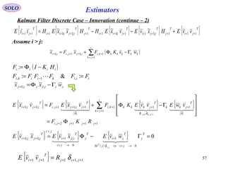
![58
Estimators
[ ] 1
11|111|11
.. −
+++++++ += j
T
jjjj
T
jjj
K
j RHPHHPK
FK
SOLO
Kalman Filter Discrete Case – Innovation (continue – 3)
Assume i > j:
1,111112,111|11,1 +++++++++++++ +Φ−+= jijjjjjiii
T
jjjjii RRKFHHHPFH δ
{ } { } { } { } { }T
ji
T
j
T
jji
T
jiii
T
j
T
jjiii
T
ji vvEHxvEvxEHHxxEHE 111|111|111|1|1111
~~~~
++++++++++++++ +−−=ιι
( )1112,12,1, +++++++ −Φ== jjjjijjiji HKIFFFF
( ){ } 1,11111|11112,1 ++++++++++++ +−−Φ= jijjj
T
jjjjjjjii RRKHPHKIFH δ
{ [ ]}
1,11
1,1111|1111|112,1
+++
+++++++++++++
=
++−Φ=
jij
jijj
T
jjjjj
T
jjjjjii
R
RRHPHKHPFH
δ
δ
{ } 1,1111
..
+++++ = jij
K
T
ji RE
FK
διι { } 01 =+iE ι
Innovation =
White Noise for
Kalman Filter Gain!!!
&
Table of Content](https://image.slidesharecdn.com/2-estimators-150110062422-conversion-gate02/85/2-estimators-57-320.jpg)
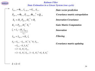

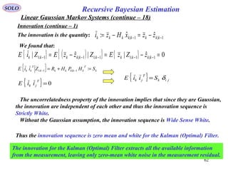
![61
1|1| ˆˆ: −− −=−= kkkkkkkk zzxHzi
Recursive Bayesian EstimationSOLO
Linear Gaussian Markov Systems (continue – 18)
Innovation
The innovation is the quantity:
We found that:
{ } ( ){ } { } 0ˆ||ˆ| 1|1:11:11|1:1 =−=−= −−−−− kkkkkkkkkk zZzEZzzEZiE
[ ][ ]{ } { } k
T
kkkkkk
T
kkk
T
kkkkkk SHPHRZiiEZzzzzE =+==−− −−−−− :ˆˆ 1|1:11:11|1|
Using the smoothing property of the expectation:
{ }{ } ( ) ( ) ( ) ( )
( )
( ) ( ) { }xEdxxpxdxdyyxpx
dxdyypyxpxdyypdxyxpxyxEE
x
X
x y
YX
x y
yxp
YYX
y
Y
x
YX
YX
==
=
=
=
∫∫ ∫
∫ ∫∫ ∫
∞+
−∞=
∞+
−∞=
∞+
−∞=
∞+
−∞=
∞+
−∞=
∞+
−∞=
∞+
−∞=
,
||
,
,
||
,
{ } { }{ }1:1 −= k
T
jk
T
jk ZiiEEiiEwe have:
Assuming, without loss of generality, that k-1 ≥ j, and innovation I (j) is
Independent on Z1:k-1, and it can be taken outside the inner expectation:
{ } { }{ } { } 0
0
1:11:1 =
== −−
T
jkkk
T
jk
T
jk iZiEEZiiEEiiE
](https://image.slidesharecdn.com/2-estimators-150110062422-conversion-gate02/85/2-estimators-60-320.jpg)
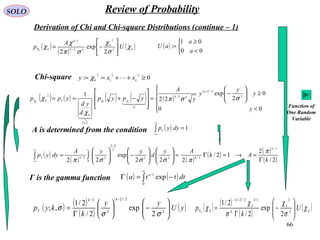
![68
SOLO Review of Probability
Derivation of Chi and Chi-square Distributions (continue – 3)
Tail probabilities of the chi-square and normal densities.
The Table presents the points on the chi-square
distribution for a given upper tail probability
{ }xyQ >= Pr
where y = χn
2
and n is the number of degrees
of freedom. This tabulated function is also
known as the complementary distribution.
An alternative way of writing the previous
equation is: { } ( )QxyQ n −=≤=− 1Pr1
2
χ
which indicates that at the left of the point x
the probability mass is 1 – Q. This is
100 (1 – Q) percentile point.
Examples
1. The 95 % probability region for χ2
2
variable
can be taken at the one-sided probability
region (cutting off the 5% upper tail): ( )[ ] [ ]99.5,095.0,0
2
2 =χ
.5 99
2. Or the two-sided probability region (cutting off both 2.5% tails): ( ) ( )[ ] [ ]38.7,05.0975.0,025.0
2
2
2
2 =χχ
.0 51
.0 975 .0 025.0 05
.7 38
3. For χ1002 variable, the two-sided 95% probability region (cutting off both 2.5% tails) is:
( ) ( )[ ] [ ]130,74975.0,025.0
2
100
2
100 =χχ
74
130](https://image.slidesharecdn.com/2-estimators-150110062422-conversion-gate02/85/2-estimators-67-320.jpg)
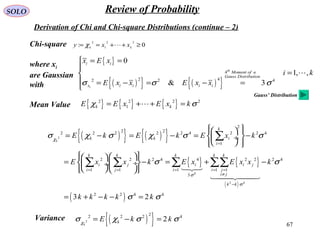
![69
SOLO Review of Probability
Derivation of Chi and Chi-square Distributions (continue – 4)
Note the skewedness of the chi-square
distribution: the above two-sided regions are
not symmetric about the corresponding means
{ } nE n =
2
χ
Tail probabilities of the chi-square and normal densities.
For degrees of freedom above 100, the
following approximation of the points on the
chi-square distribution can be used:
( ) ( )[ ]22
121
2
1
1 −+−=− nQQn Gχ
where G ( ) is given in the last line of the Table
and shows the point x on the standard (zero
mean and unity variance) Gaussian distribution
for the same tail probabilities.
In the case Pr { y } = N (y; 0,1) and with
Q = Pr { y>x }, we have x (1-Q) :=G (1-Q)
.5 99.0 51
.0 975 .0 025.0 05
.7 38](https://image.slidesharecdn.com/2-estimators-150110062422-conversion-gate02/85/2-estimators-68-320.jpg)
![71
Recursive Bayesian EstimationSOLO
Linear Gaussian Markov Systems (continue – 20)
Evaluation of Kalman Filter Consistency
A state-estimator (filter) is called consistent if its state estimation error satisfy
( ) ( ){ } ( ){ } 0|~:|ˆ ==− kkxEkkxkxE
( ) ( )[ ] ( ) ( )[ ]{ } ( ) ( ){ } ( )kkPkkxkkxEkkxkxkkxkxE TT
||~|~:|ˆ|ˆ ==−−
this is a finite-sample consistency property, that is, the estimation errors based on a
finite number of samples (measurements) should be consistent with the theoretical
statistical properties:
• Have zero mean (i.e. the estimates are unbiased).
• Have covariance matrix as calculated by the Filter.
The Consistency Criteria of a Filter are:
1. The state errors should be acceptable as zero mean and have magnitude commensurate
with the state covariance as yielded by the Filter.
2. The innovation should have the same property as in (1).
3. The innovation should be white noise.
Only the last two criteria (based on innovation) can be tested in real data applications.
The first criterion, which is the most important, can be tested only in simulations.](https://image.slidesharecdn.com/2-estimators-150110062422-conversion-gate02/85/2-estimators-70-320.jpg)
![73
Recursive Bayesian EstimationSOLO
Linear Gaussian Markov Systems (continue – 22)
Evaluation of Kalman Filter Consistency (continue – 2)
Real time (Single-Run Tests) (continue – 1)
Test 2: ( ) ( ){ } ( ){ } ( ) ( ){ } ( )kSkikiEkiEkkzkzE T
===−− &0:1|ˆ
Using the Time-Average Normalized Innovation
Squared (NIS) statistics
( ) ( ) ( )∑=
−
=
K
k
T
i kikSki
K 1
11
:ε
must have a chi-square distribution with
K nz degrees of freedom.
iK ε
Tail probabilities of the chi-square and normal densities.
The test is successful if [ ]21,rri ∈ε
where the confidence interval [r1,r2] is defined
using the chi-square distribution of iε
[ ]{ } αε −=∈ 1,Pr 21 rri
For example for K=50, nz=2, and α=0.05, using the two
tails of the chi-square distribution we get
( )
( )
==→=
==→=
→
6.250/130130925.0
5.150/7474025.0
~50
2
2
100
1
2
1002
100
r
r
i
χ
χ
χε
.0 975
.0 025
74
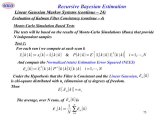
130](https://image.slidesharecdn.com/2-estimators-150110062422-conversion-gate02/85/2-estimators-72-320.jpg)
![74
Recursive Bayesian EstimationSOLO
Linear Gaussian Markov Systems (continue – 23)
Evaluation of Kalman Filter Consistency (continue – 3)
Real time (Single-Run Tests) (continue – 2)
Test 3: Whiteness of Innovation
Use the Normalized Time-Average Autocorrelation
( ) ( ) ( ) ( ) ( ) ( ) ( )
2/1
111
:
−
===
+++= ∑∑∑
K
k
T
K
k
T
K
k
T
i lkilkikikilkikilρ
In view of the Central Limit Theorem, for large K, this statistics is normal distributed.
For l≠0 the variance can be shown to be 1/K that tends to zero for large K.
Denoting by ξ a zero-mean unity-variance normal
random variable, let r1 such that
[ ]{ } αξ −=−∈ 1,Pr 11 rr
For α=0.05, will define (from the normal distribution)
r1 = 1.96. Since has standard deviation of
The corresponding probability region for α=0.05 will
be [-r, r] where
iρ K/1
KKrr /96.1/1 ==
Normal Distribution](https://image.slidesharecdn.com/2-estimators-150110062422-conversion-gate02/85/2-estimators-73-320.jpg)
![76
Recursive Bayesian EstimationSOLO
Linear Gaussian Markov Systems (continue – 25)
Evaluation of Kalman Filter Consistency (continue – 5)
Monte-Carlo Simulation Based Tests (continue – 1)
Test 1 (continue – 1):
The average, over N runs, of is( )kxiε
( ) ( )∑=
=
N
i
xix k
N
k
1
1
: εε
The test is successful if [ ]21,rrx ∈ε
where the confidence interval [r1,r2] is defined
using the chi-square distribution of iε
[ ]{ } αε −=∈ 1,Pr 21 rrx
For example for N=50, nx=2, and α=0.05, using the two
tails of the chi-square distribution we get
( )
( )
==→=
==→=
→
6.250/130130925.0
5.150/7474025.0
~50
2
2
100
1
2
1002
100
r
r
i
χ
χ
χε
Tail probabilities of the chi-square and normal densities.
.0 975
.0 025
74
130
must have a chi-square distribution with
N nx degrees of freedom.
xN ε](https://image.slidesharecdn.com/2-estimators-150110062422-conversion-gate02/85/2-estimators-75-320.jpg)
![77
Recursive Bayesian EstimationSOLO
Linear Gaussian Markov Systems (continue – 26)
Evaluation of Kalman Filter Consistency (continue – 6)
Monte-Carlo Simulation Based Tests (continue – 2)
The test is successful if [ ]21,rri ∈ε
where the confidence interval [r1,r2] is defined
using the chi-square distribution of iε
[ ]{ } αε −=∈ 1,Pr 21 rri
For example for N=50, nz=2, and α=0.05, using the two
tails of the chi-square distribution we get
( )
( )
==→=
==→=
→
6.250/130130925.0
5.150/7474025.0
~50
2
2
100
1
2
1002
100
r
r
i
χ
χ
χε
Tail probabilities of the chi-square and normal densities.
.0 975
.0 025
74
130
must have a chi-square distribution with
N nz degrees of freedom.
iN ε
Test 2: ( ) ( ){ } ( ){ } ( ) ( ){ } ( )kSkikiEkiEkkzkzE T
===−− &0:1|ˆ
Using the Normalized Innovation Squared (NIS)
statistics, compute from N Monte-Carlo runs:
( ) ( ) ( ) ( )∑=
−
=
N
j
jj
T
ji kikSki
N
k
1
11
:ε](https://image.slidesharecdn.com/2-estimators-150110062422-conversion-gate02/85/2-estimators-76-320.jpg)
![78
Recursive Bayesian EstimationSOLO
Linear Gaussian Markov Systems (continue – 27)
Evaluation of Kalman Filter Consistency (continue – 7)
Test 3: Whiteness of Innovation
Use the Normalized Sample Average Autocorrelation
( ) ( ) ( ) ( ) ( ) ( ) ( )
2/1
111
:,
−
===
= ∑∑∑
N
j
j
T
j
N
j
j
T
j
N
j
j
T
ji mimikikimikimkρ
In view of the Central Limit Theorem, for large N, this statistics is normal distributed.
For k≠m the variance can be shown to be 1/N that tends to zero for large N.
Denoting by ξ a zero-mean unity-variance normal
random variable, let r1 such that
[ ]{ } αξ −=−∈ 1,Pr 11 rr
For α=0.05, will define (from the normal distribution)
r1 = 1.96. Since has standard deviation of
The corresponding probability region for α=0.05 will
be [-r, r] where
iρ N/1
NNrr /96.1/1 ==
Normal Distribution
Monte-Carlo Simulation Based Tests (continue – 3)](https://image.slidesharecdn.com/2-estimators-150110062422-conversion-gate02/85/2-estimators-77-320.jpg)
![79
Recursive Bayesian EstimationSOLO
Linear Gaussian Markov Systems (continue – 28)
Evaluation of Kalman Filter Consistency (continue – 8)
Examples Bar-Shalom, Y, Li, X-R, “Estimation and Tracking: Principles, Techniques
and Software”, Artech House, 1993, pg.242
Monte-Carlo Simulation Based Tests (continue – 4)
Single Run, 95% probability
[ ]99.5,0∈xεTest (a) Passes if
A one-sided region is considered.
For nx = 2 we have
( ) ( )[ ] [ ]99.5,095.0,02 2
2
2
2 == χχxn
( ) ( ) ( ) ( )∑=
−
=
K
k
T
x kkxkkPkkx
K
k
1
1
|~||~1
:ε
( ) ( ) ( ) qkxkkx +−Φ= 1
See behavior of for various values of the process noise q
for filters that are perfectly matched.](https://image.slidesharecdn.com/2-estimators-150110062422-conversion-gate02/85/2-estimators-78-320.jpg)
![80
Recursive Bayesian EstimationSOLO
Linear Gaussian Markov Systems (continue – 29)
Evaluation of Kalman Filter Consistency (continue – 9)
Examples Bar-Shalom, Y, Li, X-R, “Estimation and Tracking: Principles, Techniques
and Software”, Artech House, 1993, pg.244
Monte-Carlo Simulation Based Tests (continue – 5)
Monte-Carlo, N=50, 95% probability
[ ] [ ]6.2,5.150/130,50/74 =∈xεTest (a) Passes if
( ) ( ) ( ) ( )∑=
−
=
N
j
jj
T
jx kkxkkPkkx
N
k
1
1
|~||~1
:ε(a)
( ) ( ) ( ) ( ) ( ) ( ) ( )
2/1
111
:,
−
===
= ∑∑∑
N
j
j
T
j
N
j
j
T
j
N
j
j
T
ji mimikikimikimkρ(c)
The corresponding probability region for
α=0.05 will be [-r, r] where
28.050/96.1/1 === Nrr
[ ] [ ]43.1,65.050/4.71,50/3.32 =∈iεTest (b) Passes if
( ) ( ) ( ) ( )∑=
−
=
N
j
jj
T
ji kikSki
N
k
1
11
:ε(b)
( ) ( )[ ] [ ]130,74925.0,025.02 2
100
2
100 == χχxn
( ) ( )[ ] [ ]71,32925.0,025.01 2
100
2
100 == χχzn](https://image.slidesharecdn.com/2-estimators-150110062422-conversion-gate02/85/2-estimators-79-320.jpg)
![81
Recursive Bayesian EstimationSOLO
Linear Gaussian Markov Systems (continue – 30)
Evaluation of Kalman Filter Consistency (continue – 10)
Examples Bar-Shalom, Y, Li, X-R, “Estimation and Tracking: Principles, Techniques
and Software”, Artech House, 1993, pg.245
Monte-Carlo Simulation Based Tests (continue – 6)
Example Mismatched Filter
A Mismatched Filter is tested: Real System Process Noise q = 9 Filter Model Process Noise qF=1
( ) ( ) ( ) ( )∑=
−
=
K
k
T
x kkxkkPkkx
K
k
1
1
|~||~1
:ε
( ) ( ) ( ) qkxkkx +−Φ= 1
(1) Single Run
(2) A N=50 runs Monte-Carlo with the
95% probability region
( ) ( ) ( ) ( )∑=
−
=
N
j
jj
T
jx kkxkkPkkx
N
k
1
1
|~||~1
:ε
[ ] [ ]6.2,5.150/130,50/74 =∈xεTest (2) Passes if
( ) ( )[ ] [ ]130,74925.0,025.02 2
100
2
100 == χχxn
Test Fails
Test Fails
[ ]99.5,0∈xεTest (1) Passes if
( ) ( )[ ] [ ]99.5,095.0,02 2
2
2
2 == χχxn](https://image.slidesharecdn.com/2-estimators-150110062422-conversion-gate02/85/2-estimators-80-320.jpg)
![82
Recursive Bayesian EstimationSOLO
Linear Gaussian Markov Systems (continue – 31)
Evaluation of Kalman Filter Consistency (continue – 11)
Examples Bar-Shalom, Y, Li, X-R, “Estimation and Tracking: Principles, Techniques
and Software”, Artech House, 1993, pg.246
Monte-Carlo Simulation Based Tests (continue – 7)
Example Mismatched Filter (continue -1)
A Mismatched Filter is tested: Real System Process Noise q = 9 Filter Model Process Noise qF=1
( ) ( ) ( ) qkxkkx +−Φ= 1
(3) A N=50 runs Monte-Carlo with the
95% probability region
(4) A N=50 runs Monte-Carlo with the
95% probability region
( ) ( ) ( ) ( )∑=
−
=
N
j
jj
T
ji kikSki
N
k
1
11
:ε
[ ] [ ]43.1,65.050/4.71,50/3.32 =∈iεTest (3) Passes if
( ) ( )[ ] [ ]71,32925.0,025.01 2
100
2
100 == χχzn
( ) ( ) ( ) ( ) ( ) ( ) ( )
2/1
111
:,
−
===
= ∑∑∑
N
j
j
T
j
N
j
j
T
j
N
j
j
T
ji mimikikimikimkρ
(c)
The corresponding probability region for
α=0.05 will be [-r, r] where
28.050/96.1/1 === Nrr
Test Fails
Test Fails](https://image.slidesharecdn.com/2-estimators-150110062422-conversion-gate02/85/2-estimators-81-320.jpg)
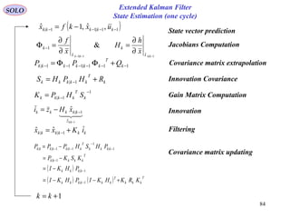
![83
Extended Kalman Filter
Sensor Data
Processing and
Measurement
Formation
Observation -
to - Track
Association
Input
Data Track Maintenance
( Initialization,
Confirmation
and Deletion)
Filtering and
Prediction
Gating
Computations
Samuel S. Blackman, " Multiple-Target Tracking with Radar Applications", Artech House,
1986
Samuel S. Blackman, Robert Popoli, " Design and Analysis of Modern Tracking Systems",
Artech House, 1999
SOLO
In the extended Kalman filter, (EKF) the state
transition and observation models need not be linear
functions of the state but may instead be (differentiable)
functions.
( ) ( ) ( )[ ] ( )kwkukxkfkx +=+ ,,1
( ) ( ) ( )[ ] ( )11,1,11 +++++=+ kkukxkhkz ν
State vector dynamics
Measurements
( ) ( ) ( ){ } ( ) ( ){ } ( )kPkekeEkxEkxke x
T
xxx =−= &:
( ) ( ) ( ){ } ( ) ( ){ } ( ) lk
T
www kQlekeEkwEkwke ,
0
&: δ=−=
( ) ( ){ } lklekeE
T
vw ,0 ∀=
=
≠
=
lk
lk
lk
1
0
,δ
The function f can be used to compute the predicted state from the previous estimate
and similarly the function h can be used to compute the predicted measurement from
the predicted state. However, f and h cannot be applied to the covariance directly.
Instead a matrix of partial derivatives (the Jacobian) is computed.
( ) ( ) ( )[ ] ( ){ } ( )[ ] ( )
( ){ }
( ) ( )
( ){ }
( ) ( )keke
x
f
keke
x
f
kekukxEkfkukxkfke wx
Hessian
kxE
T
xx
Jacobian
kxE
wx ++
∂
∂
+
∂
∂
=+−=+
2
2
2
1
,,,,1
( ) ( ) ( )[ ] ( ){ } ( )[ ] ( )
( ){ }
( ) ( )
( ){ }
( ) ( 111
2
1
111,1,11,1,11
1
2
2
1
++++
∂
∂
+++
∂
∂
=+++++−+++=+
++
kke
x
h
keke
x
h
kkukxEkhkukxkhke x
Hessian
kxE
T
xx
Jacobian
kxE
z νν
Taylor’s Expansion:](https://image.slidesharecdn.com/2-estimators-150110062422-conversion-gate02/85/2-estimators-82-320.jpg)


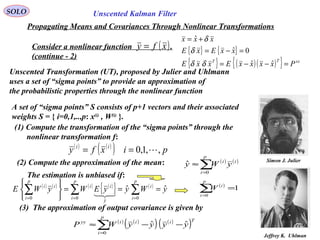
![87
Uscented Kalman FilterSOLO
When the state transition and observation models – that is, the predict and update
functions f and h (see above) – are highly non-linear, the extended Kalman filter can
give particularly poor performance [JU97]. This is because only the mean is
propagated through the non-linearity. The unscented Kalman filter (UKF) [JU97]
uses a deterministic sampling technique known as the to pick a minimal set of
sample points (called sigma points) around the mean. These sigma points are then
propagated through the non-linear functions and the covariance of the estimate is
then recovered. The result is a filter which more accurately captures the true mean
and covariance. (This can be verified using Monte Carlo sampling or through a
Taylor series expansion of the posterior statistics.) In addition, this technique
removes the requirement to analytically calculate Jacobians, which for complex
functions can be a difficult task in itself.
( ) ( ) ( )[ ] ( )kwkukxkfkx +=+ ,,1
( ) ( )[ ] ( )11,11 ++++=+ kkxkhkz ν
State vector dynamics
Measurements
( ) ( ) ( ){ } ( ) ( ){ } ( )kPkekeEkxEkxke x
T
xxx =−= &:
( ) ( ) ( ){ } ( ) ( ){ } ( ) lk
T
www kQlekeEkwEkwke ,
0
&: δ=−=
( ) ( ){ } lklekeE
T
vw ,0 ∀=
=
≠
=
lk
lk
lk
1
0
,δ
The Unscent Algorithm using ( ) ( ) ( ){ } ( ) ( ){ } ( )kPkekeEkxEkxke x
T
xxx =−= &:
Determines ( ) ( ) ( ){ } ( ) ( ){ } ( )kPkekeEkzEkzke z
T
zzz =−= &:](https://image.slidesharecdn.com/2-estimators-150110062422-conversion-gate02/85/2-estimators-86-320.jpg)
![88
Unscented Kalman FilterSOLO
( ) ( )[ ]
( )
n
n
j j
j
n
x
n
x
n
x
x
x
xx
fx
n
xxf
∂
∂
=∇⋅
∇⋅=+
∑
∑
=
∞
=
1
0
ˆ
:
!
1
ˆ
δδ
δδ
Develop the nonlinear function f in a Taylor series
around
xˆ
Define also the operator ( )[ ] ( )xf
x
xfxfD
n
n
j j
jx
n
x
n
x
x
∂
∂
=∇⋅= ∑=1
: δδδ
Propagating Means and Covariances Through Nonlinear Transformations
Consider a nonlinear function .( )xfy =
Let compute
Assume is a random variable with a probability density function pX (x) (known or
unknown) with mean and covariance
x
{ } ( ) ( ){ }Txx
xxxxEPxEx ˆˆ,ˆ −−==
( ){ } { }
( )[ ]{ } ∑ ∑∑
∑
∞
= =
∞
=
∞
=
∂
∂
=∇⋅=
=+=
0
ˆ
10
ˆ
0
!
1
!
1
!
1
ˆˆ
n
x
n
n
j j
j
n
x
n
x
n
n
x
f
x
xE
n
fxE
n
DE
n
xxfEy
x
δδ
δ δ
{ } { }
{ } ( )( ){ } xxTT
PxxxxExxE
xxExE
xxx
=−−=
=−=
+=
ˆˆ
0ˆ
ˆ
δδ
δ
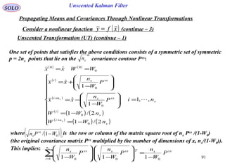
δ](https://image.slidesharecdn.com/2-estimators-150110062422-conversion-gate02/85/2-estimators-87-320.jpg)
![89
Unscented Kalman Filter
SOLO
Propagating Means and Covariances Through Nonlinear Transformations
Consider a nonlinear function .
(continue – 1)
( )xfy =
{ } { }
{ } ( )( ){ } xxTT
PxxxxExxE
xxExE
xxx
=−−=
=−=
+=
ˆˆ
0ˆ
ˆ
δδ
δ
δ
( ){ } ( )
+
∂
∂
+
∂
∂
+
∂
∂
+
∂
∂
+=
∂
∂
=+=
∑∑∑
∑∑ ∑
===
=
∞
= =
x
n
j j
jx
n
j j
jx
n
j j
j
x
n
j j
j
n
x
n
n
j j
j
f
x
xEf
x
xEf
x
xE
f
x
xExff
x
xE
n
xxfEy
xxx
xx
ˆ
4
1
ˆ
3
1
ˆ
2
1
ˆ
10
ˆ
1
!4
1
!3
1
!2
1
ˆ
!
1
ˆˆ
δδδ
δδδ
Since all the differentials of f are computed around the mean (non-random)xˆ
( )[ ]{ } ( )[ ]{ } { }( )[ ] ( )[ ]xx
xxT
xxx
TT
xxx
TT
xxx fPfxxEfxxEfxE ˆˆˆˆ
2
∇∇=∇∇=∇∇=∇⋅ δδδδδ
( )[ ]{ } { } { } 0
ˆ
1
0ˆ
1
ˆ0
ˆ =
∂
∂
=
∂
∂
=
∇⋅=∇⋅ ∑∑ ==
x
n
j j
j
x
n
j j
j
x
xxx f
x
xEf
x
xEfxEfxE
xx
δδδδ
( ){ } [ ]{ } ( ) ( )[ ] [ ]{ } [ ]{ } +++∇∇+==+= ∑
∞
=
xxxxxx
xxT
x
n
x
n
x fDEfDEfPxffDE
n
xxfEy ˆ
4
ˆ
3
ˆ
0
ˆ
!4
1
!3
1
!2
1
ˆ
!
1
ˆˆ δδδδ](https://image.slidesharecdn.com/2-estimators-150110062422-conversion-gate02/85/2-estimators-88-320.jpg)
![93
Unscented Kalman Filter
( ) ( ) ( ) ( )∑=
++
−
+∇∇+=
x
ii
n
i
xx
x
xxT
UT xfDxfD
n
W
xfPxfy
1
640
ˆ
!6
1
ˆ
!4
11
ˆ
2
1
ˆˆ δδ
( )
i
xxx
i
i
P
W
n
xxxx
−
±=±=
01
ˆˆ δ
SOLO
Propagating Means and Covariances Through Nonlinear Transformations
Consider a nonlinear function (continue – 4)( )xfy =
Unscented Transformation (UT) (continue – 3)
Unscented Algorithm:
( ) ( )
( ) ( ) ( )xfPxfP
W
n
n
W
xfP
W
n
P
W
n
n
W
xfP
W
n
P
W
n
n
W
xfD
n
W
xxTxxxT
x
n
i
T
i
xxx
i
xxxT
x
n
i
T
i
xxx
i
xxxT
x
n
i
x
x
x
xx
i
ˆ
2
1
ˆ
12
11
ˆ
112
11
ˆ
112
11
ˆ
2
11
0
0
1 00
0
1 00
0
1
20
∇∇=∇
−
∇
−
=∇
−
−
∇
−
=
∇
−
−
∇
−
=
−
∑
∑∑
=
==
δ
Finally:
We found
( ){ } [ ]{ } ( ) ( )[ ] [ ]{ } [ ]{ } +++∇∇+==+= ∑
∞
=
xxxxxx
xxT
x
n
x
n
x fDEfDEfPxffDE
n
xxfEy ˆ
4
ˆ
3
ˆ
0
ˆ
!4
1
!3
1
!2
1
ˆ
!
1
ˆˆ δδδδ
We can see that the two expressions agree exactly to the third order.](https://image.slidesharecdn.com/2-estimators-150110062422-conversion-gate02/85/2-estimators-92-320.jpg)
![94
Unscented Kalman Filter
SOLO
Propagating Means and Covariances Through Nonlinear Transformations
Consider a nonlinear function (continue – 5)( )xfy =
Unscented Transformation (UT) (continue – 4)
Accuracy of the Covariance:
( ) ( ){ } { }
( ) ( ) ( ) ( ) ( )
( ) ( )[ ] [ ]{ } [ ]{ }
( ) ( )[ ] [ ]{ } [ ]{ }
T
xxxxxx
xxT
x
xxxxxx
xxT
x
T
m
m
xx
n
n
xx
TTTyy
fDEfDEfPxf
fDEfDEfPxf
fD
m
xfDxffD
n
xfDxfE
yyyyEyyyyEP
+++∇∇+⋅
⋅
+++∇∇+−
++
++=
−=−−=
∑∑
∞
=
∞
=
ˆ
4
ˆ
3
ˆ
ˆ
4
ˆ
3
ˆ
22
!4
1
!3
1
!2
1
ˆ
!4
1
!3
1
!2
1
ˆ
!
1
ˆˆ
!
1
ˆˆ
ˆˆˆˆ
δδ
δδ
δδδδ
( ) ( ) ( ) ( ){ } ( ) ( ) ( ){ } ( ) ( ) ( )
( )
+
++
++=
∑∑
∑∑
∞
=
∞
=
∞
=
∞
=
T
m
m
x
n
n
x
T
n
n
x
T
x
T
n
n
x
T
x
T
fD
m
fD
n
E
xfxfD
n
ExfxfDExfD
n
ExfxfDExfxfxf
22
2
0
2
0
!
1
!
1
ˆˆ
!
1
ˆˆˆ
!
1
ˆˆˆˆˆ
δδ
δδδδ
](https://image.slidesharecdn.com/2-estimators-150110062422-conversion-gate02/85/2-estimators-93-320.jpg)

![96
Uscented Kalman FilterSOLO
( ) ( )∑∑ −−==
N
T
iiiz
N
ii zzPz
2
0
2
0
ψψβψβ
x
xPα
xP
zP
( )f
iβ
iβ
iψ
z
{ } [ ]xxi PxPxx ααχ −+=
Weighted
sample mean
Weighted
sample
covariance
Table of Content](https://image.slidesharecdn.com/2-estimators-150110062422-conversion-gate02/85/2-estimators-95-320.jpg)
![97
Uscented Kalman Filter
SOLO
UKF Summary
Initialization of UKF
{ } ( ) ( ){ }T
xxxxEPxEx 00000|000
ˆˆˆ −−==
{ } [ ] ( )( ){ }
=−−===
R
Q
P
xxxxEPxxEx
TaaaaaTTaa
00
00
00
ˆˆ00ˆˆ
0|0
00000|0000
[ ]TTTTa
vwxx =:
For { }∞∈ ,,1 k
Calculate the Sigma Points ( )
( )
λγ
γ
γ +=
=−=
=+=
=
−−−−
+
−−
−−−−−−
−−−−
L
LiPxx
LiPxx
xx
i
kkkk
Li
kk
i
kkkk
i
kk
kkkk
,,1ˆˆ
,,1ˆˆ
ˆˆ
1|11|11|1
1|11|11|1
1|1
0
1|1
State Prediction and its Covariance
System Definition
( ) { } { }
( ) { } { }
==+=
==+−= −−−−−−−
lkk
T
lkkkkk
lkk
T
lkkkkkk
RvvEvEvxkhz
QwwEwEwuxkfx
,
,1111111
&0,
&0,,1
δ
δ
( ) Liuxkfx k
i
kk
i
kk 2,,1,0,ˆ,1ˆ 11|11| =−= −−−−
( ) ( ) ( )
( )
Li
L
W
L
WxWx m
i
m
L
i
i
kk
m
ikk 2,,1
2
1
&ˆˆ 0
2
0
1|1| =
+
=
+
== ∑=
−−
λλ
λ
0
1
2
( )
( )( ) ( ) ( )
( )
Li
L
W
L
WxxxxWP c
i
c
L
i
T
kk
i
kkkk
i
kk
c
ikk 2,,1
2
1
&1ˆˆˆˆ 2
0
2
0
1|1|1|1|1| =
+
=+−+
+
=−−= ∑=
−−−−−
λ
βα
λ
λ](https://image.slidesharecdn.com/2-estimators-150110062422-conversion-gate02/85/2-estimators-96-320.jpg)

![100
Estimators
( ) ( ) ( ){ } ( ) ( ){ } ( )kPkekeEkxEkxke x
T
xxx =−= &:
( ) ( ) ( ) ( ) ( ) ( ) ( )
( ) ( ) ( ) ( )
( ) ( ) ( ) ( )kkvkkv
kvkxkHkz
kwkkukGkxkkx
ξ+Ψ=+
+=
Γ++Φ=+
1
1
SOLO
Kalman Filter Discrete Case & Colored Measurement Noise
Assume a discrete dynamic system
( ) ( ) ( ){ } ( ) ( ){ } ( ) lk
T
www kQlekeEkwEkwke ,
0
&: δ=−=
( ) ( ) ( ){ } ( ) ( ){ } ( ) lk
T
kRlekeEkvEkvke ,
0
&: δξξξ =−=
( ) ( ){ } { }0=lekeE
T
w ξ
=
≠
=
lk
lk
lk
1
0
,δ
Solution
Define a new “pseudo-measurement”:
( ) ( ) ( ) ( ) ( ) ( ) ( ) ( ) ( ) ( ) ( )[ ]kvkxkHkkvkxkHkzkkzk +Ψ−++++=Ψ−+= 1111:ζ
( ) ( ) ( ) ( ) ( ) ( ) ( )[ ] ( ) ( ) ( )
( )
( ) ( ) ( )kxkHkkvkkvkwkkukGkxkkH
k
Ψ−Ψ−++Γ++Φ+=
ξ
11
( ) ( ) ( ) ( )[ ]
( )
( ) ( ) ( ) ( ) ( ) ( ) ( ) ( )[ ]
( )
kkH
kkwkkHkukGkHkxkHkkkH
ε
ξ+Γ++++Ψ−Φ+= 111
*
( ) ( ) ( ) ( ) ( ) ( ) ( )kkukGkHkxkHk εζ +++= 1*](https://image.slidesharecdn.com/2-estimators-150110062422-conversion-gate02/85/2-estimators-99-320.jpg)
![101
Estimators
( ) ( ) ( ){ } ( ) ( ){ } ( )kPkekeEkxEkxke x
T
xxx =−= &:
( ) ( ) ( ) ( ) ( ) ( ) ( )
( ) ( ) ( ) ( ) ( ) ( ) ( )111211*1
1
++++++++=+
Γ++Φ=+
kkukGkHkxkHk
kwkkukGkxkkx
εζ
SOLO
Kalman Filter Discrete Case & Colored Measurement Noise
The new discrete dynamic system:
( ) ( ) ( ){ } ( ) ( ){ } ( ) lk
T
www kQlekeEkwEkwke ,
0
&: δ=−=
( ) ( ) ( ) ( ) ( ){ } ( ){ }
( ) ( ){ } ( ) ( ) ( ) ( ) ( ) ( ) lklk
TTT
kRlHlkQkkHlekeE
kEkwEkkHkke
,,11&
1:
δδ
ξε
εε
ε
++ΓΓ+=
+Γ+−=
( ) ( ){ } { }0=lekeE
T
w ξ
=
≠
=
lk
lk
lk
1
0
,δ
Solution (continue – 1)
( ) ( ) ( ) ( ) ( )kkwkkHk ξε +Γ+= 1:
( ) ( ) ( ) ( ) ( )kHkkkHkH Ψ−Φ+= 1:*
( ) ( ){ } ( ) ( ) ( ) ( ) ( )[ ]{ } ( ) ( ) lk
TTTTTTT
kHkkQllHllwkwElkwE ,11 δξε +Γ=++Γ=
To decorrelate measurements and system noises write the discrete dynamic system:
( ) ( ) ( ) ( ) ( ) ( ) ( )
( ) ( ) ( ) ( ) ( ) ( ) ( ) ( )[ ]
0
1*
1
kkukGkHkxkHkkD
kwkkukGkxkkx
εζ ++−−+
Γ++Φ=+](https://image.slidesharecdn.com/2-estimators-150110062422-conversion-gate02/85/2-estimators-100-320.jpg)
![102
Estimators
( ) ( ) ( ) ( )[ ] ( ){ } ( ) ( ) ( ) ( ) ( ) ( ) ( ) ( ) ( ) ( ) ( )[ ]kRkHkkQkkHkDkHkkQkkkkDkwkE TTTTT
++ΓΓ+−+ΓΓ==−Γ 1110εε
( ) ( ){ } ( ) ( ) ( ) ( ) ( ) ( )[ ] ( ) lklk
TTT
kRkRkHkkQkkHlkE ,, *:11 δδεε =++ΓΓ+=
SOLO
Kalman Filter Discrete Case & Colored Measurement Noise
The new discrete dynamic system:
Solution (continue – 2)
( ) ( ) ( ) ( ) ( ) ( ) ( ) ( ) ( ) ( ) ( ) ( )[ ]
( ) ( ) ( ) ( )
( ) ( ) ( ) ( ) ( ) ( ) ( )111211*1
1*1
++++++++=+
−Γ+
+−−++Φ=+
kkukGkHkxkHk
kkDkwk
kukGkHkxkHkkDkukGkxkkx
εζ
ε
ζ
To de-correlate measurement and system noises choose D (k) such that:
( ) ( ){ } ( ) ( ) ( ) ( ) ( )[ ]{ } ( ) ( ) lk
TTTTTTT
kHkkQllHllwkwElkwE ,11 δξε +Γ=++Γ=
( ) ( ) ( ) ( ) ( ) ( ) ( ) ( ) ( ) ( ) ( )[ ] 1
111
−
++ΓΓ++ΓΓ= kRkHkkQkkHkHkkQkkD TTTT
The Discrete Kalman Filter Estimator is:
( ) ( ) ( ) ( ) ( ) ( ) ( ) ( ) ( ) ( ) ( ) ( )[ ]
( ) ( ){ } 000|0ˆ
1|ˆ*|ˆ|1ˆ
xxEx
kukGkHkkxkHkkDkukGkkxkkkx
==
+−−++Φ=+ ζ
( ) ( ) ( ) ( ) ( )kHkkkHkH Ψ−Φ+= 1:*
The Aprior Covariance Update is:
( ) ( ) ( ) ( )[ ] ( ) ( ) ( ) ( )[ ] ( ) ( ) ( ) ( ) ( ) ( )
( ) 00|0
**|1*|1
PP
kDkRkDkkQkkHkDkkkPkHkDkkkP TTT
=
+ΓΓ+−Φ+−Φ=+](https://image.slidesharecdn.com/2-estimators-150110062422-conversion-gate02/85/2-estimators-101-320.jpg)
![103
Estimators
( ) ( ) ( ) ( )[ ] ( ){ } 0=−Γ kkkDkwkE T
εε
( ) ( ){ } ( ) ( ) ( ) ( ) ( ) ( )[ ] ( ) lklk
TTT
kRkRkHkkQkkHlkE ,, *:11 δδεε =++ΓΓ+=
SOLO
Kalman Filter Discrete Case & Colored Measurement Noise
The discrete dynamic system:
Solution (continue – 3)
( ) ( ) ( ) ( ) ( ) ( ) ( ) ( ) ( ) ( ) ( ) ( )[ ]
( ) ( ) ( ) ( ) ( ) ( ) ( )111211*1
1*1
++++++++=+
+−−++Φ=+
kkukGkHkxkHk
kukGkHkxkHkkDkukGkxkkx
εζ
ζ
( ) ( ) ( ) ( ) ( ) ( ) ( ) ( ) ( ) ( ) ( )[ ] 1
111
−
++ΓΓ++ΓΓ= kRkHkkQkkHkHkkQkkD TTTT
The Discrete Kalman Filter Estimator is:
( ) ( ) ( ) ( ) ( ) ( ) ( ) ( ) ( ) ( ) ( ) ( )[ ]
( ) ( ){ } 000|0ˆ
1/ˆ*|ˆ|1ˆ
xxEx
kukGkHkkxkHkkDkukGkkxkkkx
==
+−−++Φ=+ ζ
( ) ( ) ( ) ( ) ( )kHkkkHkH Ψ−Φ+= 1:*
( ) ( ) ( ) ( )[ ] ( ) ( ) ( ) ( )[ ] ( ) ( ) ( ) ( ) ( ) ( )
( ) 00|0
**|1*|1
PP
kDkRkDkkQkkHkDkkkPkHkDkkkP TTT
=
+ΓΓ+−Φ+−Φ=+
( ) ( ) ( ) ( ) ( )[ ]
( ) ( ) ( ) ( )kRkHkkPkK
kHkRkHkkPkkP
T
T
1
111
**1|11
***|11|1
−
−−−
++=+
++=++
( ) ( ) ( ) ( ) ( ) ( )[ ]kkxkHkkKkkxkkx |1ˆ1*11|1ˆ1|1ˆ ++−++++=++ ζ
Summary:](https://image.slidesharecdn.com/2-estimators-150110062422-conversion-gate02/85/2-estimators-102-320.jpg)
![104
Estimators
( ) ( ) ( ) ( ) ( ) ( ) ( ) ( ) ( ) ( ) ( ) ( )[ ]
( ) ( ){ } 000|0ˆ
1|ˆ*|ˆ|1ˆ
xxEx
kukGkHkkxkHkkDkukGkkxkkkx
==
+−−++Φ=+ ζ
SOLO
Kalman Filter Discrete Case & Colored Measurement Noise
Solution (continue – 4)
Summary:
( ) ( ) ( ) ( ) ( ) ( )[ ]kkxkHkkKkkxkkx |1ˆ1*11|1ˆ1|1ˆ ++−++++=++ ζ
( ) ( ) ( ) ( )kzkkzk Ψ−+= 1ζ
Table of Content](https://image.slidesharecdn.com/2-estimators-150110062422-conversion-gate02/85/2-estimators-103-320.jpg)
![105
Estimators
( ) ( ) ( ) ( )[ ]∫ −+−=
t
t
dtntHty
0
λλλλ s
SOLO
Optimal State Estimation in Linear Stationary Systems
The output of the Stationary Filter is given by:
Hnxn (t) is the impulse response matrix of the Stationary Filter
( ) ( )[ ] ( ) ( )[ ]{ } ( ) ( ){ } ( ) ( ) ( )tytteteteEtyttytE i
T
i
T
i −==−− yyy :
We want to estimate a vector signal that, after be corrupted by noise ,
passes trough a Linear Stationary Filter. We want to design the filter in order to
estimate the signal using only the measured filter output vector .( )tyn 1×
( )tsn 1× ( )tnn 1×
( )tsn 1×
nnx1 (t) is a noise with autocorrelation
and uncorrelated to the signal
( ) ( ) ( ){ } ( )τττ −=+= tRtntnER nn
T
nn
( ) ( ){ } ( ) ( ){ } { }0=+=+ ττ tstnEtntsE TT
( ) ( ){ } ( ) ( ){ }teteEtraceteteE TT
=
Where the trace of a square matrix A = {ai,j} is the sum of the diagonal terms
{ } ∑=
=× ==
n
i
iinjijinn aatraceAtrace
1
,,,1,, :
( ) ( ) ( )∫ −=
t
t
i dtIty
0
λλλ s
The uncorrupted signal is observed through a linear system, with impulse response
I (t) and output yi (t):
We want to choose a Stationary Filter that minimizes:](https://image.slidesharecdn.com/2-estimators-150110062422-conversion-gate02/85/2-estimators-104-320.jpg)
![106
EstimatorsSOLO
Optimal State Estimation in Linear Stationary Systems (continue – 1)
The Autocorrelation of the error is:
( ) ( ) ( ){ }
( ) ( ) ( ) ( ) ( )[ ] ( ) ( ) ( ) ( )[ ] ( )
( ) ( )[ ] ( ) ( ) ( ) ( ) ( ) ( )[ ] ( ) ( )
−+−−+−−+
−−−−−=
−++−−+
+−−−=
+=
∫∫∫∫
∫∫∫∫
∞+
∞−
∞+
∞−
∞+
∞−
∞+
∞−
∞+
∞−
∞+
∞−
∞+
∞−
∞+
∞−
22222221111111
22222221111111
ξξτξξξτξτξξξξξξξξ
ξξτξξξξτξξξξξξξξ
ττ
dtHndtHtIdntHdtHtIE
dtHndtIdntHdtIE
teteER
TTTTT
TTTT
T
ee
ss
ssss
Therefore
( ) ( ) ( )[ ] ( ) ( )[ ]
( )
( ) ( )[ ]
( ) ( ) ( )[ ]
( )
( )∫ ∫
∫ ∫
∞+
∞−
∞+
∞− −
+∞
∞−
+∞
∞− −
−+−+
−+−−+−−−=
212211
21222111
21
21
ξξξτξξξ
ξξξτξτξξξξτ
ξξ
ξξ
ddtHnnEtH
ddtHtIEtHtIR
T
R
T
TT
R
T
ee
nn
ss
ss](https://image.slidesharecdn.com/2-estimators-150110062422-conversion-gate02/85/2-estimators-105-320.jpg)
![107
Estimators
( ) ( ) ( )[ ] ( ) ( )[ ]
( )
( ) ( )[ ]
( ) ( ) ( )[ ]
( )
( )∫ ∫
∫ ∫
∞+
∞−
∞+
∞− −
+∞
∞−
+∞
∞− −
−+−+
−+−−+−−−=
212211
21222111
21
21
ξξξτξξξ
ξξξτξτξξξξτ
ξξ
ξξ
ddtHnnEtH
ddtHtIEtHtIR
T
R
T
TT
R
T
ee
nn
ss
ss
( ) ( ) ( )[ ] ( ) ( ) ( )[ ] ( ) ( )sSssssSsssS TTT
−+−−−−= HHHIHI nnssee
SOLO
Optimal State Estimation in Linear Stationary Systems (continue – 2)
The Autocorrelation of the error is:
Using the Bilateral Laplace Transform we
obtain:
( ) ( ) ( )
( ) ( )[ ] ( ) ( ) ( )[ ] ( )
( ) ( ) ( )∫ ∫
∫ ∫ ∫
∫
∞+
∞−
∞+
∞−
∞+
∞−
∞+
∞−
∞+
∞−
+∞
∞−
−+−−+
−−+−−+−−−−=
−=
212211
21222111 exp
exp
ξξξτξξξ
τξξτξτξτξξξξ
τττ
ddtHRtH
dddstHtIRtHtI
dsRsS
T
nn
TT
eeee
ss
( ) ( )[ ] ( )[ ] ( ) ( )[ ] ( ) ( )[ ] ( )[ ]
( ) ( )
( ) ( )[ ] ( ) ( )[ ] ( ) ( )[ ]
( )
∫ ∫ ∫
∫ ∫ ∫
∞+
∞−
∞+
∞−
−
∞+
∞−
+∞
∞−
+∞
∞−
−−
+∞
∞−
−+−+−−−−−−+
−+−+−−+−−−−−−−−=
222212111
122222121111
expexpexp
expexpexp
ξτξτξτξξξξξξ
ξξτξτξτξτξξξξξξξ
ddsttHsRsttH
dddsttHtIsRsttHtI
s
T
ss
TT
T
TT
H
nn
H-I
ss](https://image.slidesharecdn.com/2-estimators-150110062422-conversion-gate02/85/2-estimators-106-320.jpg)
![108
Estimators
( ) ( ) ( )[ ] ( ) ( )[ ]
( )
( ) ( )[ ]
( ) ( ) ( )[ ]
( )
( )∫ ∫
∫ ∫
∞+
∞−
∞+
∞− −
+∞
∞−
+∞
∞− −
−+−+
−+−−+−−−=
212211
21222111
21
21
ξξξτξξξ
ξξξτξτξξξξτ
ξξ
ξξ
ddtHnnEtH
ddtHtIEtHtIR
T
R
T
TT
R
T
ee
nn
ss
ss
( ) ( ) ( )[ ] ( ) ( ) ( )[ ] ( ) ( )sSssssSsssS TTT
−+−−−−= HHHIHI nnssee
SOLO
Optimal State Estimation in Linear Stationary Systems
(continue – 3)
The Autocorrelation of the error is:
Using the Bilateral Laplace Transform we finally
obtained:
where
( ) ( ) ( )
( ) ( )
( ) ( ) ( ) ( ) ( )
( ) ( ) ( )
( )
( ) ( ) ( )
ns
rrrrrrrr
rrrrrrrrrr
rrrr
rrrr
,
expexp
expexpexp
=
=−=−=
−==−−=−=
∫∫
∫∫∫
∞+
∞−
=∞+
∞−
+∞
∞−
−=+∞
∞−
−=+∞
∞−
r
sSdsRdsRsS
sSdsRdsRdsRsS
RR
TT
RR
T
ττττττ
υυυττττττ
τ
τυττ](https://image.slidesharecdn.com/2-estimators-150110062422-conversion-gate02/85/2-estimators-107-320.jpg)
![109
EstimatorsSOLO
Optimal State Estimation in Linear Stationary Systems
(continue – 4)
( )
( ) ( ){ } ( )
( ) ( ){ } ( )
( )0minminmin === τee
tH
T
tH
T
tH
RtraceteteEtraceteteE
( ) ( ) ( ) ( )∫∫
∞+
∞−=
∞+
∞−
===
j
j
ee
j
j
eeee dssS
j
dsssS
j
R
π
τ
π
τ
τ
2
1
exp
2
1
0
0
We want to find the Optimal Stationary Filter, ,that minimizes:( )tHˆ
( )
( ) ( ){ } ( )
( ) ( )
( )
( )
( ) ( )[ ] ( ) ( ) ( )[ ] ( ) ( ){ }∫
∫
∞+
∞−
∞+
∞−
−+−−−=
===
j
j
TTT
s
ee
tH
j
j
ee
tH
T
tH
dssSssssSss
j
trace
RtracedssS
j
traceteteE
HHHIHI nnss
H π
τ
π
2
1
min
0min
2
1
minmin
Using Calculus of Variation we write ( ) ( ) ( ) 0ˆ →Ψ+= εε sss HH
( ) ( ) ( )[ ] ( ) ( ) ( ) ( )[ ] ( ) ( )[ ] ( ) ( )[ ]{ }
( ) ( ) ( ) ( )[ ] ( ){ } ( ) ( )[ ] ( ) ( ) ( ){ } ( ) 0ˆˆ
2
1ˆˆ
2
1
ˆˆˆˆ
2
1
0
=−Ψ+−−+−+−−−−Ψ=
−Ψ+−Ψ++−Ψ−−−−Ψ−−
∂
∂
∫∫
∫
∞+
∞−
∞+
∞−
∞+
∞−
→
j
j
T
j
j
TTT
j
j
TTTTT
dsssSssSss
j
tracedssSsssSs
j
trace
dsssSssssssSsss
j
trace
ε
π
ε
π
εεεε
επ ε
nnssnnss
nnss
HHIHHI
HHHIHI](https://image.slidesharecdn.com/2-estimators-150110062422-conversion-gate02/85/2-estimators-108-320.jpg)
![110
EstimatorsSOLO
Optimal State Estimation in Linear Stationary Systems
(continue – 5)
( ) ( ) ( ) ( )[ ] ( ){ }
( ) ( )[ ] ( ) ( ) ( ){ } ( ) 0ˆˆ
2
1
ˆˆ
2
1
=−Ψ+−−+
−+−−−−Ψ
∫
∫
∞+
∞−
∞+
∞−
j
j
T
j
j
TTT
dsssSssSss
j
trace
dssSsssSs
j
trace
ε
π
ε
π
nnss
nnss
HHI
HHI
Since by tacking –s instead of s in one of the integrals we obtain the other, they are equal
and have zero value:
( ) ( )[ ] ( ) ( ) ( ){ } ( ) 0ˆˆ
2
1
=−Ψ+−−∫
∞+
∞−
j
j
T
dsssSssSss
j
trace ε
π
nnss HHI
This integral is zero for all if and only if:( ) 0≠−Ψ sT
( ) ( )[ ] ( ) ( ) ( ) { }0ˆˆ =+−− sSssSss nnss HHI ( ) ( ) ( )[ ] ( ) ( )sSssSsSs ssnnss IH =+ˆ
Since we can perform a Spectral Decomposition:( ) ( ) ( ) ( )[ ] T
sSsSsSsS −+−=+ nnssnnss
( ) ( ) ( ) ( )sssSsS T
−∆∆=+ nnss
( )s∆ - All poles and zeros are in L.H.P s.
- All poles and zeros are in R.H.P s.( )sT
−∆
( ) ( ) ( ) ( ) ( )sSssss T
ssIH =−∆∆ˆ ( ) ( ) ( ) ( )[ ] ( )sssSss T 1
Part
Realizable
ˆ −−
∆−∆= ssIH](https://image.slidesharecdn.com/2-estimators-150110062422-conversion-gate02/85/2-estimators-109-320.jpg)
![111
Estimators
( ) ( ) ( ) 1&1
1
3
1
3
1
3
2
==
+−
=
−
= sIsS
sss
sS nnss
( ) ( ) ( ) ( )[ ] ( )sssSss T 1
Part
Realizable
ˆ −−
∆−∆= ssIH
SOLO
Optimal State Estimation in Linear Stationary Systems (continue – 6)
Example 8.3-2 Sage, “Optimum System Control”, Prentice Hall, 1968, pp.191-192
( ) ( )
( ) ( )
ss T
s
s
s
s
s
s
s
sSsS
−∆∆
−
−
+
+
=
−
−
=+
−
=+
1
2
1
2
1
4
1
1
3
2
2
2nnss
( ) ( ) ( )[ ] ( ) ( )
Part
realizable-Un
Part
Realizable
2
2
1
1
1
21
3
2
1
1
3
sssss
s
s
ssSs T
−
+
+
=
−+
=
−
−
−
=−∆−
ssI
( )
ss
s
s
s
+
=
+
+
+
=
2
1
2
1
1
1ˆH
Solution:
( )
( ) ( ){ } ( )
( ) ( )[ ] ( ) ( ) ( )[ ] ( ) ( ){ }
( ) ( ) ( ) ( )
1
2
4
2
4
22
4
2
1
ˆˆˆˆ
2
1
2
1
minmin
=
+
=
−
=
−+
=
−+−−−==
∫∫∫
∫∫
∞+
∞−
∞+
∞−
∞+
∞−
RHPLHP
j
j
j
j
TTT
j
j
s
T
tH
ds
s
ds
s
ds
ssj
dssSssssSss
j
tracedsS
j
traceteteE
π
ππ
HHHIHI nnssee
H](https://image.slidesharecdn.com/2-estimators-150110062422-conversion-gate02/85/2-estimators-110-320.jpg)

( ) [ ][ ]( ) TT
TTT
TTT
AsIRsRsAsI
AsIAsIRAsIBQBAsI
AsIBQBAsIsssSsS
−−
−−
−−
−−−−−−=
−−−−−+−=
−−−=−∆∆=+
ΤΤ
nnss
2/12/11
1
1
where
RAARRR
ARABQB
TT
TTT
+−=−
+=
2/12/1
ΤΤ
ΤΤ
PRAR
PPPARR TTT
+−=
=−−=
2/1
2/1
&
Τ
Τ
( ) ( ) ( ) ( ) ( )
( ) ( )[ ] ( ) ( )
( ) ( )T
TT
−−=
+−−=−−−=
−−=−−=∆
−
−−−−
−−−
2/11
2/1112/111
2/112/112/11
RsAsI
RRPAsIAsIRRPRAIsAsI
RRRIsAsIRsAsIs](https://image.slidesharecdn.com/2-estimators-150110062422-conversion-gate02/85/2-estimators-111-320.jpg)
![113
Estimators
vxy
wBxAx
+=
+=
( ) ( ) ( ) ( ) ( ) [ ][ ]( ) TTT
AsIRsRsAsIsssSsS
−−
−−−−−−=−∆∆=+ ΤΤnnss
2/12/11
( ) ( ) ( )[ ] ( ) ( )
( )
( ) ( )
( )
( ) ( )
realizableUn
12/1
Realizable
1
12/11
−
−−
−∆
−−−−
−−−=
−−−−−−−=−∆
−
TT
s
TT
sS
TTT
sRBQBAsI
sRAsIAsIBQBAsIssSs
T
T
TI
ss
ss
SOLO
Optimal State Estimation in Linear Stationary Systems (continue – 8)
Example 8.5-4 Sage, “Optimum System Control”, Prentice Hall, 1968, pp.211-213
Solution (continue - 1):
( ) ( ){ } ( )
( ) ( ){ } ( )
( ) ( ){ }
( ) ( ){ } 21
21
21
2121
2121
,
0
tt
tvtwE
twtvE
ttRtvtvE
ttQtwtwE
T
T
T
T
∀
==
−=
−=
δ
δ
( ) ( ) ( ) ( ) ( ) 1&& === tItvtntxts
Let decompose the last expression in the Realizable and Un-realizable parts:
( ) ( ) ( ) ( )
TTTT
TTT
ARABQBPRPAPPAARA
PARRPRARRR
+=−−−=
−−==
−
−−
1
12/112/1
ΤΤΤΤ
{ }01
=+−+ −
BQBPRPAPPA T
( ) ( ) ( ) ( )
realizableUn
12/1
Realizable
1
realizableUn
12/1
Realizable
1
−
−−
−
−−
−−+−=−−− TTT
sRNMAsIsRBQBAsI TT
where M and N must be defined](https://image.slidesharecdn.com/2-estimators-150110062422-conversion-gate02/85/2-estimators-112-320.jpg)
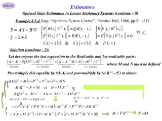
![115
Estimators
vxy
wBxAx
+=
+=
( ) ( ) ( ) ( )[ ] ( ) ( )
( ) ( ) ( )[ ]
( ) ( )
( )
sssSs
T
AsIRPAIsRRPAsIsssSss
T 1
Part
Realizable
112/12/111
Part
Realizable
ˆ
−−
∆
−−−
−∆
−−−−
−+−−=∆−∆=
ssI
ssIH
( ) ( ) ( ) ( ) ( )2/12/12/112/11 −−−
+−−=−−=∆ RPRARsAsIRsAsIs Τ
SOLO
Optimal State Estimation in Linear Stationary Systems (continue – 10)
Example 8.5-4 Sage, “Optimum System Control”, Prentice Hall, 1968, pp.211-213
Solution (continue - 3):
( ) ( ){ } ( )
( ) ( ){ } ( )
( ) ( ){ }
( ) ( ){ } 21
21
21
2121
2121
,
0
tt
tvtwE
twtvE
ttRtvtvE
ttQtwtwE
T
T
T
T
∀
==
−=
−=
δ
δ
( ) ( ) ( ) ( ) ( ) 1&& === tItvtntxts
Decompose the last expression in the Realizable and Un-realizable parts:
( ) ( ) ( )[ ] ( ) ( ) ( ) ( )
realizableUn
12/1
Realizable
2/11
realizableUn
12/1
Realizable
1
−
−−−
−
−−−
−−+−=−−−=−∆ TTTT
sRPRPAsIsRBQBAsIssSs TTI ss
PRAR +−=2/1
Τ](https://image.slidesharecdn.com/2-estimators-150110062422-conversion-gate02/85/2-estimators-114-320.jpg)
![116
Estimators
vxy
wBxAx
+=
+=
( ) ( ) ( ) ( )[ ] ( ) ( )
( ) ( ) ( )[ ]
( ) ( )
( )
sssSs
T
AsIRPAIsRRPAsIsssSss
T 1
Part
Realizable
112/12/111
Part
Realizable
ˆ
−−
∆
−−−
−∆
−−−−
−+−−=∆−∆=
ssI
ssIH
SOLO
Optimal State Estimation in Linear Stationary Systems (continue – 11)
Example 8.5-4 Sage, “Optimum System Control”, Prentice Hall, 1968, pp.211-213
Solution (continue - 4):
( ) ( ){ } ( )
( ) ( ){ } ( )
( ) ( ){ }
( ) ( ){ } 21
21
21
2121
2121
,
0
tt
tvtwE
twtvE
ttRtvtvE
ttQtwtwE
T
T
T
T
∀
==
−=
−=
δ
δ
( ) ( ) ( ) ( ) ( ) 1&& === tItvtntxts
( ) ( ) ( ) ( )[ ] ( ) ( )[ ]
( ) ( )[ ]( ){ } ( ) ( ) ( )[ ]
( ) ( )[ ]( ){ } ( ) ( )[ ]
( ) ( )[ ]{ } ( ) 111
1
111
111
1
111
1
1111
111111
1111111111ˆ
−−−
−
−−−
−−−
−
−−−
−
−−−−
−−−−−−
−−−−−−−−−−
+−=+−=
+−=−−+=
−+−=−+−=
−+−=+−−−=
RPRPAsIRPAsIRP
IAsIRPAsIAsIRP
AsIRPAsIRPRPAsIIAsI
RPAsIIRPAsIRPAsIAsIRPAsIsH
Finally: ( ) ( ) 111ˆ −−−
+−= RPRPAsIsH
{ }01
=+−+ −
BQBPRPAPPA T
where P is given by:
Continuous Algebraic
Riccati Equation (CARE)
( )xyRPxAx ˆˆˆ 1
−+= −
These solutions are particular solutions of the Kalman Filter algorithm for a
Stationary System and infinite observation time (Wiener Filter) Table of Content](https://image.slidesharecdn.com/2-estimators-150110062422-conversion-gate02/85/2-estimators-115-320.jpg)
![117
Estimators
( ) ( ) ( ) ( ) ( ) ( )twtGtxtFtxtx
td
d
+==
SOLO
Kalman Filter Continuous Time Case
Assume a continuous time linear dynamic system
( ) vxtHz +=
( ) ( ) ( ){ } ( ) ( ){ } ( )tPteteEtxEtxte
T
xxx =−= &:
( ) ( ) ( ){ } ( ) ( ){ } ( ) ( )21121
0
&: tttQteteEtwEtwte
T
www −=−= δ
( ) ( ) ( ) ( ) ( )∫+=
t
t
dztAtxttBtx
0
,ˆ,ˆ 00 τττ
( ) ( ) ( ){ } ( ) ( ){ } ( ) ( )21121
0
&: tttRteteEtvEtvte
T
vvv −=−= δ
( ) ( ){ } { }021 =teteE
T
wv
Let find a Linear Filter with the state vector that is a function of Z (t) (the history
of z for t0 < τ < t )
( )txˆ
s.t. will minimize
( ) ( )[ ] ( ) ( )[ ]{ } ( ) ( ){ } ( ) ( ) ( )txtxtxwheretxtxEtxtxtxtxEJ TT
−==−−= ˆ:~~~ˆˆ
( ){ } ( ){ }txEtxE =ˆ Unbiased Estimator
( ){ } ( ){ } ( ){ } 0ˆ~ =−= txEtxEtxE](https://image.slidesharecdn.com/2-estimators-150110062422-conversion-gate02/85/2-estimators-116-320.jpg)
![118
EstimatorsSOLO
Kalman Filter Continuous Time Case (continue – 1)
( ) ( ){ } ( ) ( ) ( ) ( ) ( ) ( ) ( ) ( ) ( ) ( )
( ) ( ) ( ){ } ( ) ( ) ( ){ } ( ) ( ) ( ) ( ){ }
( ) ( ) ( ){ } ( ) ( ) ( ) ( ){ } ( ) ( ) ( ){ } ( )
( ) ( ){ } ( ) ( ) ( ) ( ){ } ( ) ( ){ }txtxEdtxzEtAttBtxtxE
dtAztxEttBtxtxEttBttBtxtxEttB
dtxzEtAdtAztxEddtAzzEtA
txdztAtxttBtxdztAtxttBEtxtxE
T
t
t
TTT
t
t
TTTTT
t
t
T
t
t
TT
t
t
t
t
TT
T
t
t
t
t
T
+−−
−−+
−−=
−+
−+=
∫
∫
∫∫∫∫
∫∫
0
0
000 0
00
0
00
0
0
0
00
0
000000
0000
ˆ,,ˆ
,ˆ,ˆ,,ˆˆ,
,,,,
,ˆ,,ˆ,~~
τττ
λλλ
ττττττλτλλττ
ττττττ
( ) ( )[ ] ( ) ( )[ ]{ } ( ) ( ){ } ( ) ( ) ( )txtxtxwheretxtxEtxtxtxtxEJ
TT
−==−−= ˆ:~~~ˆˆ
( ){ } ( ){ } ( ){ } 0ˆ~ =−= txEtxEtxE](https://image.slidesharecdn.com/2-estimators-150110062422-conversion-gate02/85/2-estimators-117-320.jpg)
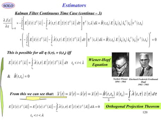
![121
EstimatorsSOLO
Kalman Filter Continuous Time Case (continue – 4)
Solution of Wiener-Hopf Equation ( ) ( ){ } ( ) ( ) ( ){ } λτλττλ <<= ∫ ttdzzEtAztxE
t
t
TT
0
0
,ˆ
Let Differentiate the Wiener-Hopf Equation relative to t:
( ) ( ){ } ( ) ( ) ( ) ( ) ( ) ( )[ ] ( ){ } ( ) ( ) ( ){ } ( ) ( ) ( ){ }
0
λλλλτ TTTTT
ztwEtGztxEtFztwtGtxtFEztx
td
d
EztxE
t
+=+=
=
∂
∂
( ) ( ) ( ){ } ( ) ( ) ( ){ } ( ) ( ) ( ){ }∫∫ ∂
∂
+=
∂
∂
t
t
TT
t
t
T
dzzEtA
t
ztzEttAdzzEtA
t 00
,ˆ,ˆ,ˆ τλττλτλττ
therefore
( ) ( ) ( ){ } ( ) ( ) ( ){ } ( ) ( ) ( ){ }∫ ∂
∂
+=
t
t
TTT
dzzEtA
t
ztzEttAztxEtF
0
,ˆ,ˆ τλττλλ
( ) ( ) ( ){ } ( ) ( ) ( ) ( )[ ] ( ){ } ( ) ( ) ( ) ( ){ } ( ) ( ) ( ){ }
0
,ˆ,ˆ,ˆ,ˆ λλλλ TTTT
ztvEttAztxEtHttAztvtxtHEttAztzEttA +=+=
Now ( ) ( ) ( ){ } ( ) ( ) ( ) ( ){ }∫=
t
t
TT
dzzEtAtFztxEtF
0
,ˆ τλττλ
( ) ( ) ( ) ( ) ( ) ( ) ( ) ( ){ } 0,ˆ,ˆ,ˆ,ˆ
0
=
∂
∂
−−∫
t
t
T
dzzEtA
t
tAtHttAtAtF τλττττ](https://image.slidesharecdn.com/2-estimators-150110062422-conversion-gate02/85/2-estimators-120-320.jpg)
![122
EstimatorsSOLO
Kalman Filter Continuous Time Case (continue – 5)
Solution of Wiener-Hopf Equation
(continue – 1)
( ) ( ){ } ( ) ( ) ( ){ } λτλττλ <<= ∫ ttdzzEtAztxE
t
t
TT
0
0
,ˆ
( ) ( ) ( ) ( ) ( ) ( ) ( ) ( ){ } 0,ˆ,ˆ,ˆ,ˆ
0 0
=
∂
∂
−−∫
≠
t
t
T
dzzEtA
t
tAtHttAtAtF τλττττ
( ) ( ) ( ) ( ) ( ) ( ) 0,ˆ,ˆ,ˆ,ˆ =
∂
∂
−− τττ tA
t
tAtHttAtAtFThis is true only if
Define ( ) ( )ttAtK ,ˆ:=
The Optimal Filter was found to be: ( ) ( ) ( )∫=
t
t
dztAtx
0
,ˆˆ τττ
( ) ( ) ( ) ( ) ( ) ( )
( )
( ) ( ) ( ) ( )
( )
( ) ( ) ( )
( ) ( ) ( ) ( ) ( )[ ] ( ) ( )
( )
( ) ( ) ( ) ( ) ( ) ( )[ ]txtHtztKtxtFdztAtHtKtFtztK
dztAtHttAtAtFtzttAdztA
t
tzttAtx
td
d
tx
t
t
t
t tKtK
t
t
ˆˆ,ˆ
,ˆ,ˆ,ˆ,ˆ,ˆ,ˆˆ
ˆ
0
00
−+=−+=
−+=
∂
∂
+=
∫
∫∫
τττ
τττττττ
Therefore the Optimal Filter is given by: ( ) ( ) ( ) ( ) ( ) ( ) ( )[ ]txtHtztKtxtFtx
td
d
ˆˆˆ −+=](https://image.slidesharecdn.com/2-estimators-150110062422-conversion-gate02/85/2-estimators-121-320.jpg)
![123
EstimatorsSOLO
Kalman Filter Continuous Time Case (continue – 6)
Solution of Wiener-Hopf Equation
(continue – 2)
( ) ( ){ } ( ) ( ) ( ){ } λτλττλ <<= ∫ ttdzzEtAztxE
t
t
TT
0
0
,ˆ
( ) ( ) ( ){ } ( ) ( ) ( ){ } ( ) ( ) ( ){ }∫ ∂
∂
+=
t
t
TTT
dzzEtA
t
ztzEttAztxEtF
0
,ˆ,ˆ τλττλλ
( ) ( ){ } ( ) ( ) ( ) ( )[ ]{ } ( ) ( ){ } ( )λλλλλλ TTTT
HxtxEvxHtxEztxE =+=Now
( ) ( ){ } ( ) ( ) ( )[ ] ( ) ( ) ( )[ ]{ } ( ) ( ) ( ){ } ( ) ( ) ( )
0→<
−+=++=
λ
λδλλλνλλνλ
t
TTTT
ttRHxtxEtHxHttxtHEztzE
( ) ( ){ } ( ) ( ) ( ){ } ( ) ( ) ( ) ( ) ( ) ( )∫+=
t
TTTTT
dGQGttxxEtxtxE
λ
γγλϕγγγγϕλϕγγγϕλ ,,,,
( ) ( ) ( )∫=
t
t
dztAtx
0
,ˆˆ τττ ( ) ( ){ } ( ) ( ) ( ){ } λτλττλ <<= ∫ ttdzzEtAztxE
t
t
TT
0
0
,ˆˆ
Must prove that
( ) ( ) ( ) ( ) ( )tRtHtPttAtK T 1
,ˆ −
==
Table of Content](https://image.slidesharecdn.com/2-estimators-150110062422-conversion-gate02/85/2-estimators-122-320.jpg)

![125
Estimators
( ) ( ) ( ) ( ) ( ) ( )twtGtxtFtxtx
td
d
+==
SOLO
Kalman Filter Continuous Time Case (Second Way)
Assume a continuous time dynamic system
( ) vxtHz +=
( ) ( ) ( ){ } ( ) ( ){ } ( )tPteteEtxEtxte
T
xxx =−= &:
( ) ( ) ( ){ } ( ) ( ){ } ( ) ( )21121
0
&: tttQteteEtwEtwte
T
www −=−= δ
( ) ( ) ( ){ } ( ) ( ){ } ( ) ( )21121
0
&: tttRteteEtvEtvte
T
vvv −=−= δ
( ) ( ){ } { }021 =teteE
T
wv
Let find a Linear Filter with the state vector that is a function of Z (t) (the history
of z for t0 < τ < t ). Assume the Linear Filter:
( )txˆ
( ) ( ) ( ) ( ) ( ) ( )tztKtxtKtxtx
td
d
+== ˆ'ˆˆ
where K’(t) and K (t) will be chosen such that:
1 The Filter is Unbiased: ( ){ } ( ){ }txEtxE =ˆ
2 The Filter will yield a maximum rate of decrease of the error by minimizing
the scalar cost function:
( ) ( )[ ] ( ) ( )[ ]{ } ( )tP
dt
d
tracetxtxtxtxE
dt
d
traceJ
KK
T
KKKK ',',',
minˆˆminmin =−−=](https://image.slidesharecdn.com/2-estimators-150110062422-conversion-gate02/85/2-estimators-124-320.jpg)
![126
Estimators
( ) ( ) ( ) ( ) ( )twtGtxtFtx +=
SOLO
Kalman Filter Continuous Time Case (Second Way – continue - 1)
( ) ( ) ( ) ( ) ( ) ( ) ( )[ ]tvtxtHtKtxtKtx ++= ˆ'ˆ
1 The Filter is Unbiased: ( ){ } ( ){ }txEtxE =ˆ
Solution
Define ( ) ( ) ( )txtxtx −= ˆ:~
( ) ( ) ( ) ( ) ( ) ( ) ( )[ ] ( ) ( ) ( ) ( ) ( )twtGtvtKtxtFtHtKtKtxtKtx −+−++= '~'~
( ){ } ( ){ } ( ){ } 0ˆ~ =−= txEtxEtxE
( ){ } ( ) ( ){ } ( ) ( ) ( ) ( )[ ] ( ){ } ( ) ( ){ } ( ) ( ){ }
0000
'~'~ twEtGtvEtKtxEtFtHtKtKtxEtKtxE −+−++=
We can see that the necessary condition for an unbiased estimator is:
( ) ( ) ( ) ( )tHtKtFtK −='
Therefore: ( ) ( ) ( ) ( )[ ] ( ) ( ) ( ) ( ) ( )twtGtvtKtxtHtKtFtx −+−= ~~
and the Unbiased Filter has the form:
( ) ( ) ( ) ( ) ( ) ( ) ( )[ ]txtHtztKtxtFtx ˆˆˆ −+=](https://image.slidesharecdn.com/2-estimators-150110062422-conversion-gate02/85/2-estimators-125-320.jpg)
![127
EstimatorsSOLO
Kalman Filter Continuous Time Case (Second Way – continue - 2)
Solution
where: ( ) ( ) ( ) ( )[ ] ( ) ( ) ( ) ( ) ( )twtGtvtKtxtHtKtFtx −+−= ~~
2 The Filter will yield a maximum rate of decrease of the error by minimizing
the scalar cost function:
( ) ( )[ ] ( ) ( )[ ]{ } ( )tP
dt
d
tracetxtxtxtxE
dt
d
traceJ
K
T
KK
minˆˆminmin =−−=
( ) ( ){ } ( ) ( ) ( )[ ] ( ) ( ){ } ( ) ( ) ( )[ ]
( ) ( ) ( ){ } ( ) ( ) ( ) ( ){ } ( )tGtwtwEtGtKtvtvEtK
tHtKtFtxtxEtHtKtFtxtxE
TTTT
TTT
++
−−= ~~~~
( ) ( ) ( ) ( )[ ] ( ) ( ) ( ) ( )[ ] ( ) ( ) ( ) ( ) ( ) ( )tGtQtGtKtRtKtHtKtFtPtHtKtFtP TTT
++−−=
To obtain the optimal K (t) that minimize J (t) we perform: ( ) { }0=
∂
∂
=
∂
∂
tPtrace
KK
J
Using the Matrix Equation: we obtain{ } ( )TT
BBAABAtrace
A
+=
∂
∂
( ) ( ) ( ) ( )[ ] ( ) ( ) ( ) ( ) { }022 =+−−=
∂
∂
=
∂
∂
tRtKtHtPtHtKtFtPtrace
KK
J T
( ) ( ) ( ) ( ) ( ) ( ) ( ) ( )[ ] 1−
+= tRtHtPtHtHtPtFtK TT
Table of Content](https://image.slidesharecdn.com/2-estimators-150110062422-conversion-gate02/85/2-estimators-126-320.jpg)

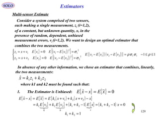
![130
EstimatorsSOLO
Multi-sensor Estimate (continue – 1)
2211
ˆ zkzkx +=
where k1 and k2 must be found such that:
1. The Estimator is Unbiased: { } { } 0~ˆ ==− xExxE 121 =+ kk
2. Minimize the Mean Square Estimation Error: ( ){ } { }2
,
2
,
~minˆmin
2121
xExxE
kkkk
=−
( ){ } ( ) ( )( )[ ]{ } ( )[ ]{ }
{ } ( ) { } ( ) { } ( ) ( )[ ]2111
2
2
2
1
2
1
2
12111
2
2
2
1
2
1
2
1
2
2111
2
2111
2
,
121min121min
1min1minˆmin
1
21
2
2
2
1
1
1121
σσρσσ
σσρσσ
kkkkvvEkkvEkvEk
vkvkExvxkvxkExxE
kk
kkkk
−+−+=
−+−+=
−+=−+−++=−
( ) ( )[ ] ( ) ( ) 0212122121 211
2
21
2
112111
2
2
2
1
2
1
2
1
1
=−+−−=−+−+
∂
∂
σσρσσσσρσσ kkkkkkk
k
21
2
2
2
1
21
2
1
12
21
2
2
2
1
21
2
2
1
2
ˆ1ˆ&
2
ˆ
σσρσσ
σσρσ
σσρσσ
σσρσ
−+
−
=−=
−+
−
= kkk
{ } ( ) 2
2
2
1
21
2
2
2
1
22
2
2
12
,
2
1~min σσ
σσρσσ
ρσσ
≤
−+
−
=xE Reduction of Covarriance Error
Estimator:](https://image.slidesharecdn.com/2-estimators-150110062422-conversion-gate02/85/2-estimators-129-320.jpg)
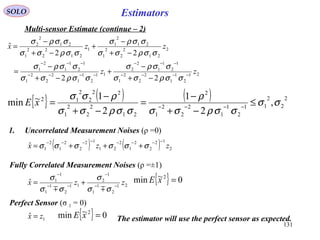
![132
EstimatorsSOLO
Multi-sensor Estimate (continue – 3)
Consider a system comprised of n sensors,
each making a single measurement, zi (i=1,2,…,n),
of a constant, but unknown quantity, x, in the
presence of random, dependent, unbiased
measurement errors, vi (i=1,2,…,n). We want to design an optimal estimator that
combines the n measurements.
{ } nivEvxz iii ,,2,10 ==+=
or
{ } { } { }[ ] { }[ ]{ } RVEVVEVEVE
v
v
v
x
z
z
z
nnnnn
nn
nn
T
V
n
UZ
n
=
=−−=
+
=
2
2211
22
2
22112
112112
2
1
2
1
2
1
0
1
1
1
σσσρσσρ
σσρσσσρ
σσρσσρσ
[ ] ZK
z
z
z
kkkzkzkzkx T
n
nnn =
=+++=
2
1
212211 ,,,ˆEstimator:](https://image.slidesharecdn.com/2-estimators-150110062422-conversion-gate02/85/2-estimators-131-320.jpg)
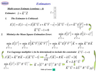
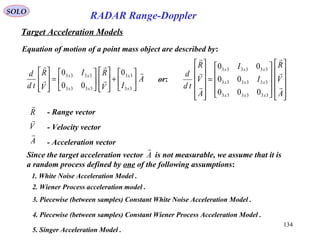
![135
SOLO
RADAR Range-Doppler
Target Acceleration Models (continue – 1)
1. White Noise Acceleration Model – Second Order Model
( ) ( ){ } ( ) ( ){ } ( )τδτ −==
+
=
tqwtwEtwEtw
IV
RI
V
R
td
d T
B
x
x
A
xx
xx
x
,0&
0
00
0
33
33
3333
3333
Discrete System ( ) ( ) ( ) ( ) ( )kwkkxkkx Γ+Φ=+1
( ) [ ]
=+===Φ ∑∫
∞
= 3333
3333
66
00
0!
1
exp:
xx
xx
x
i
ii
T
I
TII
TAITA
i
dAT ττ
2
00
00
00
00
00
0
00
0
00
0
3333
3333
3333
3333
3333
3333
3333
33332
3333
3333
≥∀
=→→
=
=→
= nA
II
A
I
A
xx
xxn
xx
xx
xx
xx
xx
xx
xx
xx
( ) ( ) ( ){ } ( ) ( ) ( )∫ −Φ−Φ=ΓΓ
T
TTT
dTBBTqkkwkwEk
0
τττ ( ) ( ){ } ( )τδτ −= tqwtwE T](https://image.slidesharecdn.com/2-estimators-150110062422-conversion-gate02/85/2-estimators-134-320.jpg)
![136
SOLO
RADAR Range-Doppler
Target Acceleration Models (continue – 2)
1. White Noise Acceleration Model (continue – 1)
( )
[ ]
( )
τ
τ
τ
d
ITI
I
I
II
TII
q
xx
xx
xx
T
x
x
xx
xx
−
−
= ∫ 3333
3333
3333
0 33
33
3333
3333 0
0
0
0
( ) ( ) ( ){ } ( ) ( ) ( ) ( ) ( ) ( )∫ −Φ−Φ=ΓΓ=ΓΓ
T
TTTTT
dTBBTqkkQkkkwkwEk
0
τττ
( )
( )[ ] ( ) ( )
( )
τ
τ
ττ
ττ
τ
d
ITI
TITI
qdITI
I
TI
q
T
xx
xx
xx
T
x
x
∫∫
−
−−
=−
−
=
0 3333
33
2
33
3333
0 33
33 2/
( ) ( ) ( )
=ΓΓ
TITI
TITI
qkkQk
xx
xxT
33
2
33
2
33
3
33
2/
2/3/
Guideline for Choice of Process Noise Intensity
The change in velocity over a sampling period T are of the order of TqQ =22
For a nearly constant velocity assumed by this model, the choice of q must be such
to give small changes in velocity compared to the actual velocity .V
](https://image.slidesharecdn.com/2-estimators-150110062422-conversion-gate02/85/2-estimators-135-320.jpg)
![137
SOLO
RADAR Range-Doppler
Target Acceleration Models (continue – 3)
2. Wiener Process acceleration model – Third Order Model
( ) ( ){ } ( ) ( ){ } ( )τδτ −==
+
=
tIqwtwEtwEtw
IA
V
R
I
I
A
V
R
td
d
x
T
B
x
x
x
A
xxx
xxx
xxx
x
33
33
33
33
333333
333333
333333
,0&0
0
000
00
00
Discrete System ( ) ( ) ( ) ( ) ( )kwkkxkkx Γ+Φ=+1
( ) [ ]
=++===Φ ∑∫
∞
=
333333
333333
2
333333
22
99
00
00
0
2/
2
1
!
1
exp:
xxx
xxx
xxx
x
i
ii
T
I
TII
TITII
TATAITA
i
dAT ττ
2
000
000
000
000
000
00
000
00
00
333333
333333
333333
333333
333333
333333
2
333333
333333
333333
>∀
=→→
=→
= nA
I
AI
I
A
xxx
xxx
xxx
n
xxx
xxx
xxx
xxx
xxx
xxx
( ) ( ) ( ){ } ( ) ( ) ( )∫ −Φ−Φ=ΓΓ
T
TTT
dTBBTqkkwkwEk
0
τττ
Since the derivative of acceleration is the jerk, this model is also called White Noise Jerk Model.
( ) ( ){ } ( )τδτ −= tIqwtwE x
T
33](https://image.slidesharecdn.com/2-estimators-150110062422-conversion-gate02/85/2-estimators-136-320.jpg)
![138
SOLO
RADAR Range-Doppler
Target Acceleration Models (continue – 4)
2. Wiener Process Acceleration Model (continue – 1)
( ) ( )
( ) [ ] ( )
( ) ( )
τ
ττ
ττ
ττ
d
ITITI
ITI
I
I
II
TII
TITII
q
xxx
xxx
xxx
xxx
T
x
x
x
xxx
xxx
xxx
−−
−
−
−−
= ∫
3333
2
33
333333
333333
333333
0
33
33
33
333333
333333
2
333333
2/
0
00
000
0
00
0
2/
( ) ( ) ( ){ } ( ) ( ) ( )∫ −Φ−Φ=ΓΓ
T
TTT
dTBBTqkkwkwEk
0
τττ
( )
( ) ( ) ( )[ ]
( ) ( ) ( )
( ) ( ) ( )
( ) ( )
τ
ττ
τττ
τττ
ττττ
τ
d
ITITI
TITITI
TITITI
qdITITI
I
TI
TI
q
T
xxx
xxx
xxx
xxx
T
x
x
x
∫∫
−−
−−−
−−−
=−−
−
−
=
0
3333
2
33
33
2
33
3
33
2
33
3
33
4
33
3333
2
33
0
33
33
2
33
2/
2/
2/2/4/
2/
2/
( ) ( ) ( )
=ΓΓ
TITITI
TITITI
TITITI
qkkQk
xxx
xxx
xxx
T
33
2
33
3
33
2
33
3
33
4
33
3
33
4
33
5
33
2/6/
2/3/8/
6/8/20/
Guideline for Choice of Process Noise Intensity
The change in acceleration over a sampling period T are of the order of TqQ =33
For a nearly constant acceleration assumed by this model, the choice of q must be such
to give small changes in velocity compared to the actual acceleration .A
( ) ( ){ } ( )τδτ −= tIqwtwE x
T
33](https://image.slidesharecdn.com/2-estimators-150110062422-conversion-gate02/85/2-estimators-137-320.jpg)
![139
SOLO
RADAR Range-Doppler
Target Acceleration Models (continue – 5)
3. Piecewise (between samples) Constant White Noise Acceleration Model – 2nd
Order
( ) ( ){ } ,0&
0
00
0
33
33
3333
3333
=
+
=
twEtw
IV
RI
V
R
td
d
B
x
x
A
xx
xx
x
Discrete System
( ) ( ) ( ) ( ) ( ) ( ) ( ) ( ){ } ( ) ( ) ( ) kl
TTT
lqkllwkwEkkwkkxkkx δΓΓ=ΓΓΓ+Φ=+ 01
( ) [ ]
=+===Φ ∑∫
∞
= 3333
3333
66
00
0!
1
exp:
xx
xx
x
i
ii
T
I
TII
TAITA
i
dAT ττ
2
00
00
00
00
00
0
00
0
00
0
3333
3333
3333
3333
3333
3333
3333
33332
3333
3333
≥∀
=→→
=
=→
= nA
II
A
I
A
xx
xxn
xx
xx
xx
xx
xx
xx
xx
xx
( ) ( ) ( ) ( )
( )
( )
( ) ( )kw
TI
TI
kw
I
d
I
TII
dkTwBTkwk
x
x
x
x
T
xx
xx
T
kw
=
−
=+−Φ=Γ ∫∫ 33
2
33
33
33
0 3333
3333
0
2/0
0
: τ
τ
τττ
](https://image.slidesharecdn.com/2-estimators-150110062422-conversion-gate02/85/2-estimators-138-320.jpg)
![140
SOLO
RADAR Range-Doppler
Target Acceleration Models (continue – 6)
3. Piecewise (between samples) Constant White Noise Acceleration Model
( ) ( ) ( ){ } ( ) ( ) ( ) [ ] klxx
x
x
kl
TTT
TITI
TI
TI
qlqkllwkwEk δδ 33
2
33
33
2
33
00 2/
2/
=ΓΓ=ΓΓ
( ) ( ) ( ){ } ( ) lk
xx
xxTT
TITI
TITI
qllwkwEk ,2
33
3
33
3
33
4
33
0
2/
2/2/
δ
=ΓΓ
Guideline for Choice of Process Noise Intensity
For this model q should be of the order of maximum acceleration magnitude aM.
A practical range is 0.5 aM ≤ q ≤ aM.](https://image.slidesharecdn.com/2-estimators-150110062422-conversion-gate02/85/2-estimators-139-320.jpg)
![141
SOLO
RADAR Range-Doppler
Target Acceleration Models (continue – 7)
4. Piecewise (between samples) Constant Wiener Process Acceleration Model
( ) ( ){ } 0&0
0
000
00
00
33
33
33
333333
333333
333333
=
+
=
twEtw
IA
V
R
I
I
A
V
R
td
d
B
x
x
x
A
xxx
xxx
xxx
x
Discrete System
( ) ( ) ( ) ( ) ( ) ( ) ( ) ( ){ } ( ) ( ) ( ) lk
TTT
lqkllwkwEkkwkkxkkx ,01 δΓΓ=ΓΓΓ+Φ=+
( ) [ ]
=++===Φ ∑∫
∞
=
333333
333333
2
333333
22
99
00
00
0
2/
2
1
!
1
exp:
xxx
xxx
xxx
x
i
ii
T
I
TII
TITII
TATAITA
i
dAT ττ
2
000
000
000
000
000
00
000
00
00
333333
333333
333333
333333
333333
333333
2
333333
333333
333333
≥∀
=→→
=→
= nA
I
AI
I
A
xxx
xxx
xxx
n
xxx
xxx
xxx
xxx
xxx
xxx
( ) ( ) ( ) ( )
( )
( ) ( )
( ) ( ) ( )kw
I
TI
TI
kwd
I
TII
TITII
dkTwBTkwk
x
x
xT
x
x
x
xxx
xxx
xxxT
kw
=
−
−−
=+−Φ=Γ ∫∫
33
33
2
33
0
33
33
33
333333
333333
2
333333
0
2/
0
0
0
00
0
2/
: ττ
ττ
τττ
](https://image.slidesharecdn.com/2-estimators-150110062422-conversion-gate02/85/2-estimators-140-320.jpg)
![142
SOLO
RADAR Range-Doppler
Target Acceleration Models (continue – 8)
4. Piecewise (between samples) Constant White Noise acceleration model
( ) ( ) ( ){ } ( ) ( ) ( ) [ ] lkxxx
x
x
x
lk
TTT
ITITI
I
TI
TI
qlqkllwkwEk ,3333
2
33
33
33
2
33
0,0 2/
2/
δδ
=ΓΓ=ΓΓ
( ) ( ) ( ){ } ( ) lk
xxx
xxx
xxx
TT
ITITI
TITITI
TITITI
qllwkwEk ,
3333
2
33
33
2
33
3
33
2
33
3
33
4
33
0
2/
2/
2/2/2/
δ
=ΓΓ
Guideline for Choice of Process Noise Intensity
For this model q should be of the order of maximum acceleration increment over a
sampling period ΔaM.
A practical range is 0.5 ΔaM ≤ q ≤ ΔaM.](https://image.slidesharecdn.com/2-estimators-150110062422-conversion-gate02/85/2-estimators-141-320.jpg)
![143
SOLO
Singer Target Model
R.A. Singer, “Estimating Optimal Tracking Filter Performance for Manned Maneuvering
Target”, IEEE Trans. Aerospace & Electronic Systems”, Vol. AES-6, July 1970,
pp. 437-483
The target acceleration is modeled as a zero-mean random process with exponential
autocorrelation
( ) ( ) ( ){ } T
etataER mTT
ττ
σττ /2 −
=+=
where σm
2
is the variance of the target acceleration and τT is the time constant of its
autocorrelation (“decorrelation time”).
The target acceleration is assumed to:
1. Equal to the maximum acceleration value amax
with probability pM and to – amax
with the same probability.
2. Equal to zero with probability p0.
3. Uniformly distributed between [-amax, amax]
with the remaining probability 1-2 pM – p0 > 0.
( ) ( ) ( )[ ] ( ) ( ) ( )[ ]
max
0
maxmax0maxmax
2
21
0
a
pp
aauaauppaaaaap M
M
−−
−−+++−++= δδδ
RADAR Range-Doppler
Target Acceleration Models (continue – 9)](https://image.slidesharecdn.com/2-estimators-150110062422-conversion-gate02/85/2-estimators-142-320.jpg)
![144
SOLO
Singer Target Model (continue 1)
( ) ( ) ( )[ ] ( ) ( ) ( )[ ]
max
0
maxmax0maxmax
2
21
0
a
pp
aauaauppaaaaap M
M
−−
−−+++−++= δδδ
{ } ( ) ( ) ( )[ ] ( ){ }
( ) ( )[ ]
( ) ( )[ ] 0
22
21
0
2
21
0
max
max
max
max
max
max
max
max
2
max
0
0maxmax
max
0
maxmax
0maxmax
=
−−
+⋅++−=
−−
−−++
+−++==
+
−
−
−−
∫
∫∫
a
a
M
M
a
a
M
a
a
M
a
a
a
a
pp
ppaa
daa
a
pp
aauaau
daappaaaadaapaaE δδδ
{ } ( ) ( ) ( )[ ] ( ){ }
( ) ( )[ ]
( ) ( )[ ]
( )0
2
max
3
max
02
max
2
max
2
max
0
maxmax
2
0maxmax
22
41
3
32
21
2
21
0
max
max
max
max
max
max
max
max
pp
a
a
a
pp
paa
daa
a
pp
aauaau
daappaaaadaapaaE
M
a
a
M
M
a
a
M
a
a
M
a
a
−+=
−−
+−++=
−−
−−++
+−++==
+
−
−
−−
∫
∫∫ δδδ
{ } { } ( )0
2
max
0
222
41
3
pp
a
aEaE Mm −+=−=
σ
Use
( ) ( ) ( )
max0max
00
max
max
aaa
afdaafaa
a
a
+≤≤−
=−∫−
δ
RADAR Range-Doppler
Target Acceleration Models (continue – 10)](https://image.slidesharecdn.com/2-estimators-150110062422-conversion-gate02/85/2-estimators-143-320.jpg)
![145
SOLO
Target Acceleration Approximation by a Markov Process
w (t) x (t)
( )tF
( )tG ∫
x (t)
( ) ( ) ( ) ( ) ( ) ( )twtGtxtFtxtx
td
d
+== Given a Continuous Linear System:
Let start with the first order linear system describing Target Acceleration :
( ) ( ) ( )twtata T
T
T +−=
τ
1
( ) ( ) T
T
tt
a ett τ
φ /
0
0
, −−
=
( ) ( ){ }[ ] ( ) ( ){ }[ ]{ } ( )τδττ −=−− tqwEwtwEtwE
( ) ( ){ }[ ] ( ) ( ){ }[ ]{ } ( )ttRtaEtataEtaE TT aaTTTT ,τττ +=−+−+
( ) ( ){ }[ ] ( ) ( ){ }[ ]{ } ( )τττ +=+−+− ttRtaEtataEtaE TT aaTTTT ,
( ) ( ){ }[ ] ( ) ( ){ }[ ]{ } ( ) ( ) 2
, TTTTT aaaaaTTTT ttRtVtaEtataEtaE σ===−−
( ) ( ) ( ) ( ) ( ) ( ) ( ) ( )tGtQtGtFtVtVtFtV
td
d TT
xxx ++= ( ) ( ) qtVtV
td
d
TTTT aa
T
aa +−=
τ
2
( ) ( )00 ,
1
, tttt
td
d
TT a
T
a φ
τ
φ −=
where
Target Acceleration Models (continue – 11)
RADAR Range-Doppler](https://image.slidesharecdn.com/2-estimators-150110062422-conversion-gate02/85/2-estimators-144-320.jpg)
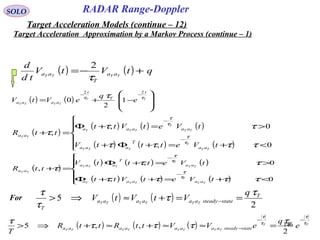
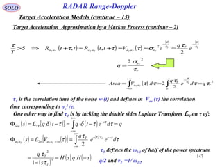
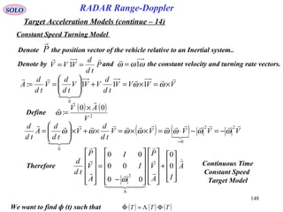
![149
SOLO
Constant Speed Turning Model (continuous – 1)
RADAR Range-Doppler
Target Acceleration Models (continue – 15)
A
B
C
O
θ
φφ
nˆ
v
1v
Let rotate the vector around by a large angle
, to obtain the new vector
→
= OAPT
nˆ
Tωθ =
→
=OBP
From the drawing we have:
→→→→
++== CBACOAOBP
TPOA
=
→
( )( )θcos1ˆˆ −××=
→
TPnnAC
Since direction of is: ( ) ( ) φsinˆˆ&ˆˆ TTT PPnnPnn
=××××
and it’s length is:
AC
→
( )θφ cos1sin −TP
( ) θsinˆ TPnCB
×=
→
Since has the direction and the
absolute value
CB
→
TPn
׈
θφsinsinv
( )( ) ( ) θθ sinˆcos1ˆˆ TTT PnPnnPP
×+−××+=
( ) ( )[ ] ( ) ( )TPnTPnnPP TTT ωω sinˆcos1ˆˆ
×+−××+=
We will find ф (T) by direct computation of a rotation:](https://image.slidesharecdn.com/2-estimators-150110062422-conversion-gate02/85/2-estimators-148-320.jpg)
![150
SOLO
Constant Speed Turning Model (continuous – 2)
RADAR Range-Doppler
Target Acceleration Models (continue – 16)
( ) ( ) ( ) ( )TPnnTPn
Td
Pd
V TT ωωωω
sinˆˆcosˆ ××+×==
( ) ( )TT PnTVV
×=== ˆ0 ω
( ) ( ) ( ) ( )TPnnTPn
Td
Vd
A TT ωωωω cosˆˆsinˆ 22
××+×−==
( ) ( )TT PnnTAA
××=== ˆˆ0 2
ω
( ) ( )[ ]
( ) ( )
( ) ( )
+−=
+=
−++=
−
−−
TT
TT
TTT
ATVTA
ATVTV
ATVTPP
ωωω
ωωω
ωωωω
cossin
sincos
cos1sin
1
21
( ) ( ) ( ) ( )[ ]TPnnTPnPP TTT ωω cos1ˆˆsinˆ −××+×+=
](https://image.slidesharecdn.com/2-estimators-150110062422-conversion-gate02/85/2-estimators-149-320.jpg)
![151
SOLO
Constant Speed Tourning Model (continuous – 3)
RADAR Range-Doppler
Target Acceleration Models (continue – 17)
( ) ( )[ ]
( ) ( )
( ) ( )
+−=
+=
−++=
−
−−
TT
TT
TTT
ATVTA
ATVTV
ATVTPP
ωωω
ωωω
ωωωω
cossin
sincos
cos1sin
1
21
( ) ( )[ ]
( ) ( )
( ) ( )
( )
−
−
=
Φ
−
−−
T
T
T
T
A
V
P
TT
TT
TTI
A
V
P
ωωω
ωωω
ωωωω
cossin0
sincos0
cos1sin
1
21
Discrete Time
Constant Speed
Target Model](https://image.slidesharecdn.com/2-estimators-150110062422-conversion-gate02/85/2-estimators-150-320.jpg)
![152
SOLO
Constant Speed Tourning Model (continuous – 4)
RADAR Range-Doppler
Target Acceleration Models (continue – 18)
( )
( ) ( )[ ]
( ) ( )
( ) ( )
−
−
=Φ −
−−
TT
TT
TTI
T
ωωω
ωωω
ωωωω
cossin0
sincos0
cos1sin
1
21
( )
( ) ( )[ ]
( ) ( )
( ) ( )
−
−−
=Φ −
−−
−
TT
TT
TTI
T
ωωω
ωωω
ωωωω
cossin0
sincos0
cos1sin
1
21
1
( )
( ) ( )
( ) ( )
( ) ( )
−−
−=Φ
−
TT
TT
TT
T
ωωωω
ωωω
ωωω
sincos0
cossin0
sincos0
2
1
We want to find Λ (t) such that
( ) ( ) ( )TTT ΦΛ=Φ therefore ( ) ( ) ( )TTT 1−
ΦΦ=Λ
( ) ( ) ( )
( ) ( )
( ) ( )
( ) ( )
( ) ( )[ ]
( ) ( )
( ) ( )
−
−−
−−
−=ΦΦ=Λ −
−−−
−
TT
TT
TTI
TT
TT
TT
TTT
ωωω
ωωω
ωωωω
ωωωω
ωωω
ωωω
cossin0
sincos0
cos1sin
sincos0
cossin0
sincos0
1
21
2
1
1
−
=
00
100
010
2
ω
We recovered the transfer matrix for the continuous
case.](https://image.slidesharecdn.com/2-estimators-150110062422-conversion-gate02/85/2-estimators-151-320.jpg)
![154
SOLO
Fixed Wing Air Vehicle Acceleration Model (continue – 1)
RADAR Range-Doppler
Target Acceleration Models (continue – 20)
( ) WWWWWWWWWWWWW
L
W
W
L
zVqyVrxVxzryqxpVxV
td
xd
VxV
td
Vd
11111111
1
1 −+=×+++=+=
( )
( ) ( )
( )
( )
+−
+
+
=
+
−
−
=
−
=
=
=
gCl
gC
gCf
gC
L
DT
m
Vq
Vr
V
A
A
A
td
Vd
A
W
L
W
L
W
L
W
L
W
W
zW
yW
xWW
L
W
3,3
3,20
3,1
1
0
0
0
1
( )[ ]
( ) VgCr
VgClq
W
LW
W
LW
/3,2
/3,3
=
−=
Therefore the Air vehicle Acceleration in it’s Wind (W) Coordinates is given by:
( ) ( )WWWWWWWWWWWWWW
I
xqyplyrzqfzlxfzlxfzlxf
td
Ad
A 1111111111: +−−+−+−=−+−==
⋅⋅
( ) ( )
( ) gCAmLl
gCAmDTf
W
LzW
W
LxW
3,3/:
3,1/:
+−==
−=−=
( )
−−
+
−
=
W
WW
W
W
qfl
rfpl
qlf
A
](https://image.slidesharecdn.com/2-estimators-150110062422-conversion-gate02/85/2-estimators-153-320.jpg)
![155
SOLO
Fixed Wing Air Vehicle Acceleration Model (continue – 2)
RADAR Range-Doppler
Target Acceleration Models (continue – 21)
( )[ ]
( ) VgCr
VgClq
W
LW
W
LW
/3,2
/3,3
=
−=
We found:
( )
mLl
mDTf
/:
/:
=
−=
( )
−−
+
−
=
W
WW
W
W
qfl
rfpl
qlf
A
, pW are pilot controlled and are modeled as zero mean
random variables
lf ,
( )
{ }
( )[ ]
( )[ ] ( )
( )[ ] ( )[ ]
−−−
−
−−
=
−
−
=
VgClgCV
VgCgCV
VgCll
qf
rf
ql
AE
W
L
W
L
W
L
W
L
W
L
W
W
W
W
/3,31,3
/2,31,3
/3,3
( )
{ } ( )
( )[ ]
( )[ ] ( )
( )[ ] ( )[ ]
−−−
−
−−
=
gClgCV
gCgCV
gCll
C
V
AE
W
L
W
L
W
L
W
L
W
L
TW
L
L
3,31,3
2,31,3
3,3
1
( ) ( )
{ } ( )
−
=−
l
pl
f
CAEA W
TW
L
LL
( ) ( )
{ } ( ) ( )
{ } ( ) W
L
l
p
f
TW
L
T
LLLL
ClCAEAAEAE W
=
−
−
2
22
2
00
00
00
σ
σ
σ](https://image.slidesharecdn.com/2-estimators-150110062422-conversion-gate02/85/2-estimators-154-320.jpg)
![156
SOLO
RADAR Range-Doppler
Target Acceleration Models (continue – 22)
( )tA
IA
V
R
I
I
A
V
R
td
d
B
x
x
x
A
xxx
xxx
xxx
x
+
=
33
33
33
333333
333333
333333
0
0
000
00
00
Discrete System
( ) ( ) ( ) ( ) ( )kAkkxkkx
Γ+Φ=+1
( ) [ ]
=++===Φ ∑∫
∞
=
333333
333333
2
333333
22
99
00
00
0
2/
2
1
!
1
exp:
xxx
xxx
xxx
x
i
ii
T
I
TII
TITII
TATAITA
i
dAT ττ
2
000
000
000
000
000
00
000
00
00
333333
333333
333333
333333
333333
333333
2
333333
333333
333333
≥∀
=→→
=→
= nA
I
AI
I
A
xxx
xxx
xxx
n
xxx
xxx
xxx
xxx
xxx
xxx
( ) ( ) ( ) ( )
( )
( ) ( )
( ) ( ) ( )kA
TI
TI
TI
kAd
II
TII
TITII
dkTABTkAk
x
x
xT
x
x
x
xxx
xxx
xxxT
kA
=
−
−−
=+−Φ=Γ ∫∫
33
33
3
33
0
33
33
33
333333
333333
2
333333
0
2/
6/
0
0
00
0
2/
: ττ
ττ
τττ
Fixed Wing Air Vehicle Acceleration Model (continue – 3)](https://image.slidesharecdn.com/2-estimators-150110062422-conversion-gate02/85/2-estimators-155-320.jpg)
![158
SOLO
RADAR Range-Doppler
Target Acceleration Models (continue – 24)
Fixed Wing Air Vehicle Acceleration Model (continue – 5)
We need to defined the matrix CL
W
.
For this we see that is along and is alongWx1 Wz1V
L
( )
( ) ( )
( )
( )
( )
( )
=
==
3,1
2,1
1,1
0
0
1
11
W
L
W
L
W
L
TW
L
W
W
TW
L
L
W
C
C
C
CxCx
( )
( ) ( )
( )
( )
( )
( )
=
==
3,3
2,3
1,3
1
0
0
11
W
L
W
L
W
L
TW
L
W
W
TW
L
L
W
C
C
C
CzCz
Therefore ( ) ( ) ( ) ( )
( ) ( )
[ ]LLVLVLVVC LLLLTW
L ///
×=
LWW zgzlxfA 111 +−=
Azgxfzl LWW
−+= 111
( ) ( ) ( ) ( )[ ] ( ) ( ) gCVgCACACACgCAf
W
L
W
L
V
z
W
Ly
W
Lx
W
L
W
LxW 3,13,13,12,11,13,1 −=−++=−=
( )
( ) ( ) ( )[ ] ( )
( )
( )
( )
−
+
−++=
z
y
x
W
L
W
L
W
L
W
L
V
z
W
Ly
W
Lx
W
L
L
W
A
A
A
g
C
C
C
gCACACACzl
1
0
0
3,1
2,1
1,1
3,13,12,11,11
( ) ( ) ( )[ ] [ ] 222
/3,12,11,1 zyxzyx
W
L
W
L
W
L VVVVVVCCC ++=
( ) ( ) ( )[ ] [ ] VAVAVAVACACACAV zzyyxxz
W
Ly
W
Lx
W
LzW /3,12,11,1 ++=++==](https://image.slidesharecdn.com/2-estimators-150110062422-conversion-gate02/85/2-estimators-157-320.jpg)
![159
SOLO
RADAR Range-Doppler
Target Acceleration Models (continue – 25)
Fixed Wing Air Vehicle Acceleration Model (continue – 6)
CL
W,
f, l , qW, rW Computation from Vectors
( ) ( )LL
AV
,
Compute:
( ) ( ) ( )[ ] [ ] 222
/3,12,11,1 zyxzyx
W
L
W
L
W
L VVVVVVCCC ++= 1
( ) ( ) ( )[ ] [ ] VAVAVAVACACACAV zzyyxxz
W
Ly
W
Lx
W
LzW /3,12,11,1 ++=++==2
( ) ( )
( )
( )
( )
( )
( )
( )
Abs
AgVVVgVV
AVVVgVV
AVVVgVV
C
C
C
z
L
L
zzz
yyz
xxz
W
L
W
L
W
L
L
W
L
/
//
//
//
3,3
2,3
1,3
1
−+−
−−
−−
=
==
3
( )[ ] ( )[ ] ( )[ ]222
//////: zzzyyzxxz AgVVVgVVAVVVgVVAVVVgVVAbs −+−+−−+−−=
( ) ( ) ( ) ( )
( ) ( )
[ ]LLVLVLVVC LLLLTW
L ///
×=4
( )
( ) ( )
( )
( )
×=
LL
VLVL
VV
C
L
LL
L
W
L
/
/
/
or
( )[ ]
( ) VgCr
VgClq
W
LW
W
LW
/3,2
/3,3
=
−=( )
( ) ( ) ( )[ ] ( ) gCACACACl
gCVf
W
Lz
W
Ly
W
Lx
W
L
W
L
3,33,32,31,3
3,1
+++−=
−=
5](https://image.slidesharecdn.com/2-estimators-150110062422-conversion-gate02/85/2-estimators-158-320.jpg)
![160
SOLO
RADAR Range-Doppler
Target Acceleration Models (continue – 26)
Ballistic Missile Acceleration Model
( )g
1
mTF
m
A A ++=
( ) ( )
( ) ( ) ( )[ ]WLWDref
WWA
zVCxVCS
VZ
zVLxVDF
1,1,
2
1,1,
2
αα
ρ
αα
−−=
−−=
- Drag and Lift Aerodynamic Forces as
functions of angle of attack α and
air pressure ρ (Z)
BxTT 1=
- Thrust Force
For small angle of attack α the wind (W) coordinates and body (B) coordinates
coincide, therefore we will use only wind (W) and Local Level Local North (L)
coordinates, related by:
W
LC - Transformation Matrix from (L) to (W)
L
T
L z
R
zgg 11 2
µ
==
where - earth gravitation
( )
LWW zgz
m
L
x
m
DT
A 111 +−
−
≈
Force Equations
WxVV 1=
- Air Vehicle Velocity Vector
MV
Bx
By
Bz
Wz
Wy
Wx
α
β
α
β
Bp
Wp
Bq
WqBr
Wr](https://image.slidesharecdn.com/2-estimators-150110062422-conversion-gate02/85/2-estimators-159-320.jpg)
![162
SOLO
RADAR Range-Doppler
Target Acceleration Models (continue – 28)
Ballistic Missile Acceleration Model (continue – 2)
CL
W0
Computation:
( ) 2/1222
ZYXV ++=( )
=
Z
Y
X
V L
Define: ψ - trajectory azimuth angle ( )XY ,tan 1−
=ψ
γ - trajectory pitch angle ( )221
,tan YXZ += −
γ
[ ] [ ]
−
−
=
−
−
==
γψγψγ
ψψ
γψγψγ
ψψ
ψψ
γγ
γγ
ψγ
cossinsincossin
0cossin
sinsincoscoscos
100
0cossin
0sincos
cos0sin
010
sin0cos
32
0W
LC](https://image.slidesharecdn.com/2-estimators-150110062422-conversion-gate02/85/2-estimators-161-320.jpg)
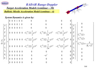
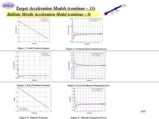
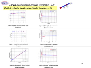
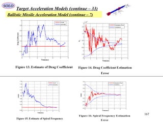
![171171
EstimatorsSOLO
Kalman Filter for Filtering Position and Velocity Measurements
Assume a Cartezian Model of a Non-maneuvering Target:
w
x
x
x
x
td
d
wx
xx
BA
+
=
⇒
=
=
1
0
00
10
( ) [ ]
=+=+++++==Φ ∫ 10
1
!
1
2
1
exp: 22
0
T
TAITA
n
TATAIdAT nn
T
ττ
2
00
00
00
00
00
10
00
10
00
10 2
≥∀
=→→
=
=→
= nAAA n
+
=+=
2
1
v
v
x
x
vxz
Measurements
( ) ( ) ( )
=
−−
=
−
=−Φ=Γ ∫∫ T
TT
d
T
dBTT
T
TT
2/2/
1
0
10
1
:
2
0
2
00 τ
τ
τ
τ
ττ
Discrete System
+=
Γ+Φ=
++++
+
1111
1
kkkk
kkkkk
vxHz
wxx
{ }
{ }
==+
=
==
+
=
++++++
ΓΦ
+
+
kj
V
PT
jkkkk
H
k
kjq
T
jkkkkk
vvERvxz
wwEQw
T
T
x
T
x
k
kk
δ
σ
σ
δσ
2
2
111111
2
2
1
0
0
&
10
01
&
2/
10
1
1
](https://image.slidesharecdn.com/2-estimators-150110062422-conversion-gate02/85/2-estimators-170-320.jpg)
![172172
EstimatorsSOLO
Kalman Filter for Filtering Position and Velocity Measurements (continue – 1)
The Kalman Filter:
( )
−+=
Φ=
+++++++
+
kkkkkkkkk
kkkkk
xHzKxx
xx
|1111|11|1
||1
ˆˆˆ
ˆˆ
T
kkk
T
kkkkkk QPP ΓΓ+ΦΦ=+ ||1
[ ]TT
T
T
Tpp
ppT
pp
pp
P q
kkkk
kk 2/
2/
1
01
10
1 22
2
|2212
1211
|12212
1211
|1 σ
+
=
=
+
+
[ ]TT
T
T
Tpp
TppTpp
pp
pp
P q
kkkk
kk 2/
2/
1
01 22
2
|2212
22121211
|12212
1211
|1 σ
+
++
=
=
+
+
( ) ( )
( ) kkqq
qq
q
kkkk
kk
TpTTpp
TTppTTpTpp
TT
TT
pTpp
TppTpTpp
pp
pp
P
|
22
22
23
2212
23
2212
242
221211
2
23
34
|222212
2212
2
221211
|12212
1211
|1
2/
2/4/2
2/
2/4/2
+++
+++++
=
+
+
+++
=
=
+
+
σσ
σσ
σ](https://image.slidesharecdn.com/2-estimators-150110062422-conversion-gate02/85/2-estimators-171-320.jpg)
![173173
EstimatorsSOLO
Kalman Filter for Filtering Position and Velocity Measurements (continue – 2)
The Kalman Filter:
( )
−+=
Φ=
+++++++
+
kkkkkkkkk
kkkkk
xHzKxx
xx
|1111|11|1
||1
ˆˆˆ
ˆˆ
[ ] 1
11|111|11
−
+++++++ += k
T
kkkk
T
kkkk RHPHHPK
( )( ) kkP
V
VP
kk
V
P
pp
pp
ppppp
pp
pp
pp
pp
pp
|1
2
1112
12
2
22
2
12
2
22
2
112212
1211
|1
1
2
2212
12
2
11
2212
1211 1
++
−
+−
−+
−++
=
+
+
=
σ
σ
σσσ
σ
( )( )
( )
( ) kkPV
PV
VP pppppppp
pppppppp
ppp
/1
2
12
2
11222212
2
122212
2
1212111211
2
12
2
2211
2
12
2
22
2
11
1
+
−+−+
++−−+
−++
=
σσ
σσ
σσ
( )( )
( )
( ) kkPV
PV
VP pppp
pppp
ppp
|1
2
12
2
1122
2
12
2
12
2
12
2
2211
2
12
2
22
2
11
1
+
−+
−+
−++
=
σσ
σσ
σσ](https://image.slidesharecdn.com/2-estimators-150110062422-conversion-gate02/85/2-estimators-172-320.jpg)
![174174
EstimatorsSOLO
Kalman Filter for Filtering Position and Velocity Measurements (continue – 2)
The Kalman Filter:
[ ] 1
11/111/11
−
+++++++ += k
T
kkkk
T
kkkk RHPHHPK
( )( )
( )
( ) kkPV
PV
VP pppp
pppp
ppp
/1
2
12
2
1122
2
12
2
12
2
12
2
2211
2
12
2
22
2
11
1
+
−+
−+
−++
=
σσ
σσ
σσ
2
23
34
/222212
2212
2
221211
/12212
1211
/1
2/
2/4/2
q
kkkk
kk
TT
TT
pTpp
TppTpTpp
pp
pp
P σ
+
+
+++
=
=
+
+
( ) ( )
( ) ( ) ( )
( ) ( ) ( ) ( ) 4///2//1
2////1
//1
422
22121111
32
221212
22
2222
TTkkpTkkpkkpkkp
TTkkpkkpkkp
Tkkpkkp
q
q
q
σ
σ
σ
+++=+
++=+
+=+](https://image.slidesharecdn.com/2-estimators-150110062422-conversion-gate02/85/2-estimators-173-320.jpg)
![175175
EstimatorsSOLO
Kalman Filter for Filtering Position and Velocity Measurements (continue – 3)
The Kalman Filter:
[ ] 1
11/111/11
−
+++++++ += k
T
kkkk
T
kkkk RHPHHPK
( )
( ) ( )
( ) ( ) ( )
+−−−
−−
=+
++++++++
+++
+ T
kkk
T
kkkkk
kkk
k
KRKHKIPHKI
PHKI
P
11111111
111
1
( )( )
( )
kkPV
PV
VPk
k
ppppp
pppp
pppKK
KK
K
/1
2
222211
2
12
2
12
2
12
2
12
2
2211
2
12
2
22
2
1112221
1211
1
1
++
+
++−
−+
−++
=
=
σσ
σσ
σσ
( )( )
( )
( ) kkVPV
PPV
VP
kk
pp
pp
ppp
HKI
/1
22
11
2
12
2
12
22
22
2
12
2
22
2
11
11
1
+
++
+−
−+
−++
=−
σσσ
σσσ
σσ
( )
( )( )
( )
( ) kkVPV
PPV
VP
kkkkkk
pp
pp
pp
pp
ppp
PHKIP
/1
2212
1211
22
11
2
12
2
12
22
22
2
12
2
22
2
11
/1111/1
1
+
+++++
+−
−+
−++
=−=
σσσ
σσσ
σσ
( )( )
( )[ ]
( )[ ]
=
=
−+
−+
−++
=
+
++
++
2
2
12221
1211
1
2
22
2
21
2
12
2
11
/1
2
1222
2
11
222
12
22
12
2
1211
2
22
2
2
12
2
22
2
11
1/1
0
0
1
V
P
k
kVP
VP
kkPVVP
VPVP
VP
kk
KK
KK
KK
KK
pppp
pppp
ppp
P
σ
σ
σσ
σσ
σσσσ
σσσσ
σσ](https://image.slidesharecdn.com/2-estimators-150110062422-conversion-gate02/85/2-estimators-174-320.jpg)
![176
Estimators
w
x
x
x
x
td
d
BA
+
=
1
0
00
10
SOLO
We want to find the steady-state form of the filter for
Assume that only the position measurements are available
x
x
- position
- velocity
[ ] { } { } kjjkkk
k
kkkk RvvEvEv
x
x
vxHz δ==+
=+= ++++
+
++++ 1111
1
1111 0&01
Discrete System
+=
Γ+Φ=
++++
+
1111
1
kkkk
kkkkk
vxHz
wxx
{ }
[ ] { }
==+=
==
+
=
++++++
ΓΦ
+
+
kjP
T
jkkkk
H
k
kjw
T
jkkkkk
vvERvxz
wwEQw
T
T
x
T
x
k
kk
δσ
δσ
2
111111
2
2
1
&01
&
2/
10
1
1
α - β (2-D) Filter with Piecewise Constant White Noise Acceleration Model](https://image.slidesharecdn.com/2-estimators-150110062422-conversion-gate02/85/2-estimators-175-320.jpg)
![177
EstimatorsSOLO
Discrete System
+=
Γ+Φ=
++++
+
1111
1
kkkk
kkkkk
vxHz
wxx
{ }
[ ] { }
==+=
==
+
=
++++++
ΓΦ
+
+
kjP
T
jkkkk
H
k
kjw
T
jkkkkk
vvERvxz
wwEQw
T
T
x
T
x
k
kk
δσ
δσ
2
111111
2
2
1
&01
&
2/
10
1
1
( ) ( ) ( ) ( ) ( )11/111 +++++=+ kRkHkkPkHkS
T
( ) ( ) ( ) ( ) 1
11/11
−
+++=+ kSkHkkPkK T
When the Kalman Filter reaches the steady-state
( ) ( )
=++=
∞→∞→
2212
1211
1/1lim/lim
pp
pp
kkPkkP
kk
( )
=+
∞→
2212
1211
/1lim
mm
mm
kkP
k
[ ] 2
11
2
1212
1211
0
1
01 PP m
mm
mm
S σσ +=+
=
( )
( )
+
+
=
+
=
= 2
1112
2
1111
2
112212
1211
12
11
/
/1
0
1
P
P
P mm
mm
mmm
mm
k
k
K
σ
σ
σ
( ) ( ) ( )[ ] ( )kkPkHkKIkkP /1111/1 +++−=++[ ]
−
=
2212
1211
12
11
2212
1211
01
10
01
mm
mm
k
k
pp
pp
( ) ( )
( )
( ) ( )
( ) ( )
+−+
++
=
−−
−−
= 2
11
2
1222
2
1112
2
2
1112
22
1111
2
1212221211
12111111
//
//
1
11
PPP
PPPP
mmmmm
mmmm
mkmmk
mkmk
σσσ
σσσσ
α - β (2-D) Filter with Piecewise Constant White Noise Acceleration Model (continue – 1)](https://image.slidesharecdn.com/2-estimators-150110062422-conversion-gate02/85/2-estimators-176-320.jpg)
![178
EstimatorsSOLO
From ( ) ( ) ( ) ( ) ( )kQkkkPkkkP
T
+ΦΦ=+ //1
we obtain ( ) ( ) ( ) ( )[ ] ( )kkQkkPkkkP T−−
Φ−+Φ= /1/ 1
( ) ( )
=++=
∞→∞→
2212
1211
1/1lim/lim
pp
pp
kkPkkP
kk
( )
=+
∞→
2212
1211
/1lim
mm
mm
kkP
k
T
TTT
TT
mm
mmT
pp
pp
Q
w
−−
ΦΦ
−
−
−
=
1
01
2/
2/4/
10
1 2
23
34
2212
1211
2212
1211
1
σ
For Piecewise (between samples) Constant White Noise acceleration model
( ) ( )
( )
−+−
+−−+−
=
−−
−−
22
22
23
2212
23
2212
24
22
2
1211
1212221211
12111111
2/
2/4/2
1
11
ww
ww
TmTmTm
TmTmTmTmTm
mkmmk
mkmk
σσ
σσ
22
1212
23
221211
24
22
2
121111
2/
4/2
w
w
w
Tmk
TmTmk
TmTmTmk
σ
σ
σ
=
−=
+−=
α - β (2-D) Filter with Piecewise Constant White Noise Acceleration Model (continue – 2)](https://image.slidesharecdn.com/2-estimators-150110062422-conversion-gate02/85/2-estimators-177-320.jpg)
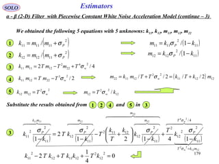
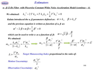
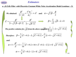
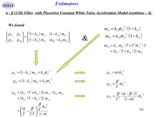
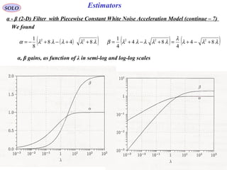
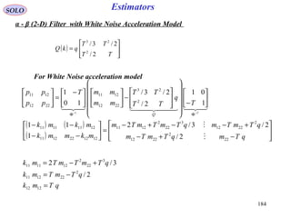
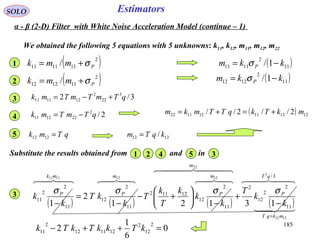
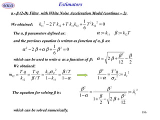
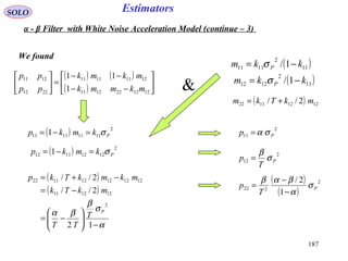
![188
Estimators
w
x
x
x
x
x
x
td
d
BA
+
=
1
0
0
000
100
010
SOLO
We want to find the steady-state form of the filter for
Assume that only the position measurements are available
[ ] { } { } kjjkkk
k
kkkk RvvEvEv
x
x
x
vxHz δ==+
=+= ++++
+
++++ 1111
1
1111 0&001
Discrete System
+=
Γ+Φ=
++++
+
1111
1
kkkk
kkkkk
vxHz
wxx { }
[ ] { }
==+=
==
+
=
++++++
ΓΦ
+
+
kjP
T
jkkkk
H
k
kjw
T
jkkkkk
vvERvxz
wwEQwT
T
xT
TT
x
k
kk
δσ
δσ
2
111111
2
22
1
&001
&
1
2/
100
10
2/1
1
α – β - γ (3-D) Filter with Piecewise Constant Wiener Process Acceleration Model
x
x
x
- position
- velocity
- acceleration](https://image.slidesharecdn.com/2-estimators-150110062422-conversion-gate02/85/2-estimators-187-320.jpg)
![189
SOLO
Estimators
Piecewise (between samples) Constant White Noise acceleration model
( ) ( ) ( ){ } ( ) ( ) ( ) [ ]12/
1
2/
2
2
00 TTT
T
qlqkllwkwEk kl
TTT
=ΓΓ=ΓΓ δ
( ) ( ) ( ){ } ( )
=ΓΓ
12/
2/
2/2/2/
2
23
234
0
TT
TTT
TTT
qllwkwEk TT
Guideline for Choice of Process Noise Intensity
For this model q should be of the order of maximum acceleration increment over a
sampling period ΔaM.
A practical range is 0.5 ΔaM ≤ q ≤ ΔaM.
α – β - γ (3-D) Filter with Piecewise Constant Wiener Process Acceleration Model
(continue – 1)](https://image.slidesharecdn.com/2-estimators-150110062422-conversion-gate02/85/2-estimators-188-320.jpg)
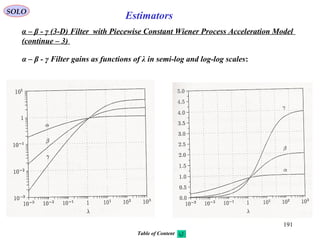
![194
SOLO Estimators
Continuous Filter-Smoother Algorithms
Problem - Choose w(t) and x(t0) to minimize:
( ) ( ) { }∫ −− −+−+−+−=
f
f
t
t
QRSffS
dtwwxHzxtxxtxJ
0
11
0
2222
00
2
1
2
1
2
1
subject to: ( ) ( ) ( ) ( ) ( ) ( )twtGtxtFtxtx
td
d
+==
( ) ( ) ( ) ( )tvtxtHtz +=
and given: ( ) ( ) ( ) ( ) ( ) ( ) ( )tGtFtHtQtRSSxxtwtz ff ,,,,,,,,,, 00
Smoothing Interpretation
are noisy observations of Hx, i.e.:
v(t) is zero-mean white noise vector with density matrix R(t).
w(t) are random forcing functions, i.e., white noise vector with prior mean w(t)
and density matrix Q(t).
(x0, P0) are mean and covariance of initial state vector from independent observations
before test
(xf, Pf) are mean and covariance of final state vector from independent observations
after test
( ) ( )[ ] ( )[ ]T
S
xtxSxtxxtx 00000
2
00
2
1
:
2
1
0
−−=−where](https://image.slidesharecdn.com/2-estimators-150110062422-conversion-gate02/85/2-estimators-193-320.jpg)
![195
SOLO Estimators
Continuous Filter-Smoother Algorithms
Solution to the Problem :
( ) nHamiltonia:H =++−+−= −− wGxFwwxHz T
QR
λ
22
11
2
1
2
1
Euler-Lagrange equations:
( )
( )
+−=
∂
∂
=
−−=
∂
∂
−=
−
−
GQww
w
H
FHRxHz
x
H
TT
TTT
λ
λλ
1
1
0
Two-Point Boundary Value Problem
Define:
( ) ( )[ ]
( ) ( )[ ]
−=
∂
∂
=
−−=
∂
∂
−=
f
T
ff
t
f
T
T
t
T
Sxtx
x
J
t
Sxtx
x
J
t
f
λ
λ 0000
0
Boundary equations:
λT
GQww −=
( ) ( )
( ) ( )
( ) ( ) ( ) ( )ttPtxtx
tSxtx
tSxtx
FF
tt
SP
ffff
λ
λ
λ
−=⇒
−=
+= →
=−
−
−
0
1
00:
0
1
000
1
zRHFxHRH TTT 11 −−
+−−= λλ
( ) ( )
w
T
GQwGxFtx λ−+=
td
d
( )
( )
( )
( )
+
−−
−
=
−−
zRH
wG
t
tx
FHRH
GQGF
t
tx
TTT
T
11
λλ
Assumed solution
Forward](https://image.slidesharecdn.com/2-estimators-150110062422-conversion-gate02/85/2-estimators-194-320.jpg)
![196
SOLO Estimators
Continuous Filter-Smoother Algorithms
Solution to the Problem (continue – 1) :
Differentiate and use previous equations
( )
( )
( )
( )
+
−−
−
=
−−
zRH
wG
t
tx
FHRH
GQGF
t
tx
TTT
T
11
λλ
( ) ( ) ( ) ( ) ( ) ( )
( ) ( ) ( ) ( ) ( ) ( ) ( )[ ]
( )
( ) ( )
( ) ( ) ( )[ ]
( )
( ) ( )twGtGQGttPtxF
tzRHtFttPtxHRHtPttPtx
ttPttPtxtx
T
tx
FF
TT
tx
FF
T
FFF
FFF
+−−=
+−−−⋅−−=
−−=
−−
λλ
λλλ
λλ
11
( ) ( ) ( ) ( ) ( )[ ] ( )
( ) ( ) ( ) ( ) ( )[ ] ( )ttPHRHtPtPFFtPtP
twGtxHtzRHtPtxFtx
F
T
FF
T
FF
F
T
FFF
λ1
1
−
−
+−−=
−−−−
( ) ( ) ( ) ( )ttPtxtx FF λ−=First Way, Assumption 1 .
( ) ( )
( ) ( )
+=
−=
−
−
ffff tSxtx
tSxtx
λ
λ
1
0
1
000
or](https://image.slidesharecdn.com/2-estimators-150110062422-conversion-gate02/85/2-estimators-195-320.jpg)
![197
SOLO Estimators
Continuous Filter-Smoother Algorithms
Solution to the Problem (continue – 2) :
( )
( )
( )
( )
+
−−
−
=
−−
zRH
wG
t
tx
FHRH
GQGF
t
tx
TTT
T
11
λλ
( ) ( ) ( ) ( ) ( )[ ] ( )
( ) ( ) ( ) ( ) ( )[ ] ( )ttPHRHtPtPFFtPtP
twGtxHtzRHtPtxFtx
F
T
FF
T
FF
F
T
FFF
λ1
1
−
−
+−−=
−−−−
( ) ( )
( ) ( )
+=
−=
−
−
ffff tSxtx
tSxtx
λ
λ
1
0
1
000
We want to have xF(t) independent on λ(t). This is obtain by choosing
( ) ( ) ( ) ( ) ( ) ( ) 1
000
1 −−
==−+= SPtPtPHRHtPtPFFtPtP FF
T
FF
T
FF
( ) ( ) ( ) ( ) ( )[ ] ( ) ( )
( ) ( ) 1
00
: −
=
=+−+=
RHtPtK
xtxtwGtxHtztKtxFtx
T
FF
FFFFF
Therefore
Let substitute the results in the equation( )tλ
( ) ( ) ( ) ( )[ ] ( ) ( )
( )
( ) ( ) ( )[ ]
( ) ( ) ( ) ( ) ( ) ( ) ( ) ( )[ ] ( )[ ]ffFffFfffffFffFffF
F
T
T
RHtP
F
TT
FF
T
xtxPtPttPxtxtxtxttP
txHtzRHtHKF
tzRHtFttPtxHRHt
T
F
−+=⇒−−=−=
−+
−−=
+−−−=
−
−
−−
−
1
1
11
1
λλλ
λ
λλλ
( ) ( ) ( ) ( )ttPtxtx FF λ−=First Way, Assumption 1 (continue – 1) .](https://image.slidesharecdn.com/2-estimators-150110062422-conversion-gate02/85/2-estimators-196-320.jpg)
![198
SOLO Estimators
Continuous Filter-Smoother Algorithms
Problem - Choose w(t) and x(t0) to minimize:
( ) ( ) { }∫ −− −+−+−+−=
f
f
t
t
QRSffS
dtwwxHzxtxxtxJ
0
11
0
2222
00
2
1
2
1
2
1
subject to: ( ) ( ) ( ) ( ) ( ) ( )twtGtxtFtxtx
td
d
+==
( ) ( ) ( ) ( )tvtxtHtz +=
Forward Covariance Filter
( ) ( ) ( ) ( ) ( )[ ] ( ) ( )
( ) ( ) ( ) ( ) ( ) ( )
( ) ( ) 1
00
1
00
: −
−
=
=−+=
=+−+=
RHtPtKwhere
PtPtPHRHtPtPFFtPtP
xtxtwGtxHtztKtxFtx
T
FF
FF
T
FF
T
FF
FFFFF
Store xF(t) and PF(t)
Backward Information Filter (τ = tf – t)
( )[ ] ( ) ( ) ( )[ ] ( ) ( )[ ] ( )[ ]ffFffFfF
TT
F xtxPtPttxHtzRHtHtKF
td
d
d
d
−+=−−−−=−=
−− 11
λλ
λ
τ
λ
Summary of First Assumption – Forward then Backward Algorithms
where = Estimate of w(t)( ) ( ) ( )tGQtwtw T
λ−=
= Smoothed Estimate of x(t)( ) ( ) ( )tPtxtx FF λ−=](https://image.slidesharecdn.com/2-estimators-150110062422-conversion-gate02/85/2-estimators-197-320.jpg)
![199
SOLO Estimators
Continuous Filter-Smoother Algorithms
Solution to the Problem :
( ) nHamiltonia:H =++−+−= −− wGxFwwxHz T
QR
λ
22
11
2
1
2
1
Euler-Lagrange equations:
( )
( )
+−=
∂
∂
=
−−=
∂
∂
−=
−
−
GQww
w
H
FHRxHz
x
H
TT
TTT
λ
λλ
1
1
0
Two-Point Boundary Value Problem
Define:
( ) ( )[ ]
( ) ( )[ ]
−=
∂
∂
=
−−=
∂
∂
−=
f
T
ff
t
f
T
T
t
T
Sxtx
x
J
t
Sxtx
x
J
t
f
λ
λ 0000
0
Boundary equations:
λT
GQww −=
zRHFxHRH TTT 11 −−
+−−= λλ
( ) ( )[ ]
( ) ( )[ ]
( ) ( ) ( ) ( )txtStt
Sxtx
x
J
t
Sxtx
x
J
t
FF
f
T
ff
t
f
T
T
t
T
f
−=⇒
−=
∂
∂
=
−−=
∂
∂
−=
λλ
λ
λ 0000
0
Second Way, Assumption 2:
Forward](https://image.slidesharecdn.com/2-estimators-150110062422-conversion-gate02/85/2-estimators-198-320.jpg)
![200
SOLO Estimators
Continuous Filter-Smoother Algorithms
Solution to the Problem (continue – 1) :
Differentiate and use previous equations
( )
( )
( )
( )
+
−−
−
=
−−
zRH
wG
t
tx
FHRH
GQGF
t
tx
TTT
T
11
λλ
( ) ( ) ( ) ( ) ( ) ( )
( ) ( ) ( ) ( ) ( ) ( ) ( ) ( )[ ] ( ){ }
( ) ( ) ( ) ( )[ ] ( )tzRHtxtStFtxHRH
twGtxtStGQGtxFtStxtSt
txtStxtStt
T
FF
TT
FF
T
FFF
FFF
11 −−
+−−−=
+−−⋅−−=
−−=
λ
λλ
λλ
( ) ( ) ( ) ( ) ( ) ( ) ( )
( ) ( ) ( ) ( ) ( )[ ] ( )txHRHtSGQGtStSFFtStS
twGtStzRHtGQGtStFt
T
F
T
FF
T
FF
F
T
F
T
FF
T
F
1
1
−
−
−+++=
−−++
λλλ
( ) ( ) ( ) ( )txtStt FF −=λλSecond Way, Assumption 2
( ) ( )[ ]
( ) ( )[ ]
−=
−−=
f
T
fff
T
TT
Sxtxt
Sxtxt
λ
λ 0000
or](https://image.slidesharecdn.com/2-estimators-150110062422-conversion-gate02/85/2-estimators-199-320.jpg)
![201
SOLO Estimators
Continuous Filter-Smoother Algorithms
Solution to the Problem (continue – 1) :
( )
( )
( )
( )
+
−−
−
=
−−
zRH
wG
t
tx
FHRH
GQGF
t
tx
TTT
T
11
λλ
( ) ( ) ( ) ( ) ( ) ( ) ( )
( ) ( ) ( ) ( ) ( )[ ] ( )txHRHtSGQGtStSFFtStS
twGtStzRHtGQGtStFt
T
F
T
FF
T
FF
F
T
F
T
FF
T
F
1
1
−
−
−+++=
−−++
λλλ
( ) ( ) ( ) ( )txtStt FF −=λλSecond Way, Assumption 2
( ) ( )[ ]
( ) ( )[ ]
−=
−−=
f
T
fff
T
TT
Sxtxt
Sxtxt
λ
λ 0000
We want to have λF(t) independent on x(t). This is obtain by choosing
( ) ( ) ( ) ( ) ( ) ( )
( ) ( )tSQGtC
StSHRHtCQtCtSFFtStS
F
T
F
F
T
FFF
T
FF
=
=+−−−= −−
:
00
11
Therefore
( ) ( )[ ] ( ) ( ) ( ) ( ) ( ) 000
1
xSttwGtStzRHttCGFt FF
T
F
T
FF =+++−= −
λλλ
Let substitute the results in the equation( )tx
( ) ( ) ( ) ( ) ( )[ ] ( )
( )[ ] ( ) ( ) ( )[ ]
( ) ( ) ( ) ( )[ ] ( ) ( )[ ] ( )[ ]fffFffFfffFfFffff
F
T
F
FF
T
xStStStxtxtStxStxS
tQGtwGtxtCGF
twGtxtStGQGtxFtx
++=⇒−+=
−++=
+−−=
−
λλ
λ
λ
1
](https://image.slidesharecdn.com/2-estimators-150110062422-conversion-gate02/85/2-estimators-200-320.jpg)
![( ) ( )[ ] ( ) ( ) ( ) ( ) ( )
( ) ( ) ( ) ( ) ( ) ( )
( ) ( )tSQGtC
StSHRHtCQtCtSFFtStS
xSttwGtStzRHttCGFt
F
T
F
F
T
FFF
T
FF
FF
T
F
T
FF
=
=+−−−=
=+++−=
−−
−
:
00
11
000
1
λλλ
202
SOLO Estimators
Continuous Filter-Smoother Algorithms
Problem - Choose w(t) and x(t0) to minimize:
( ) ( ) { }∫ −− −+−+−+−=
f
f
t
t
QRSffS
dtwwxHzxtxxtxJ
0
11
0
2222
00
2
1
2
1
2
1
subject to: ( ) ( ) ( ) ( ) ( ) ( )twtGtxtFtxtx
td
d
+==
( ) ( ) ( ) ( )tvtxtHtz +=
Forward InformationFilter
Store λF(t) and SF(t)
Backward Information Smoother (τ = tf – t)
Summary of Second Assumption – Forward then Backward Algorithms
( )[ ] ( ) ( ) ( )[ ] ( ) ( )[ ] ( )[ ]fffFffFfF
T
F xStStStxtQGtwGtxtCGF
td
xd
d
xd
++=⇒−−+−=−=
−
λλ
τ
1
where = Estimate of w(t)( ) ( ) ( )tGQtwtw T
λ−=
= Smoothed Estimate of x(t)( ) ( ) ( )tPtxtx FF λ−=](https://image.slidesharecdn.com/2-estimators-150110062422-conversion-gate02/85/2-estimators-201-320.jpg)
![203
SOLO Estimators
Continuous Filter-Smoother Algorithms
Solution to the Problem :
( ) nHamiltonia:H =++−+−= −− wGxFwwxHz T
QR
λ
22
11
2
1
2
1
Euler-Lagrange equations:
( )
( )
+−=
∂
∂
=
−−=
∂
∂
−=
−
−
GQww
w
H
FHRxHz
x
H
TT
TTT
λ
λλ
1
1
0
Two-Point Boundary Value Problem
Define:
( ) ( )[ ]
( ) ( )[ ]
−=
∂
∂
=
−−=
∂
∂
−=
f
T
ff
t
f
T
T
t
T
Sxtx
x
J
t
Sxtx
x
J
t
f
λ
λ 0000
0
Boundary equations:
λT
GQww −=
zRHFxHRH TTT 11 −−
+−−= λλ
( )[ ] ( ) ( )
( ) ( ) ( )
( ) ( ) ( ) ( )ttPtxtx
tPtSxtx
tPtSxtx
BB
ffffff
λ
λλ
λλ
+=⇒
==−
==−−
−
−
1
000
1
000
Third Way, Assumption 3:
Backward](https://image.slidesharecdn.com/2-estimators-150110062422-conversion-gate02/85/2-estimators-202-320.jpg)
![204
SOLO Estimators
Continuous Filter-Smoother Algorithms
Solution to the Problem (continue – 1) :
Differentiate and use previous equations
( )
( )
( )
( )
+
−−
−
=
−−
zRH
wG
t
tx
FHRH
GQGF
t
tx
TTT
T
11
λλ
( ) ( ) ( ) ( ) ( ) ( )
( ) ( ) ( ) ( ) ( ) ( ) ( )[ ] ( ) ( ){ }
( ) ( ) ( )[ ] ( ) ( )twGtGQGttPtxF
tzRHtFttPtxHRHtPttPtx
ttPttPtxtx
T
BB
TT
BB
T
BBB
BBB
+−+=
+−+−⋅++=
++=
−−
λλ
λλλ
λλ
11
( ) ( ) ( ) ( ) ( )[ ] ( )
( ) ( ) ( ) ( ) ( )[ ] ( )ttPHRHtPGQGFtPtPFtP
twGtxHtzRHtPtFxtx
B
T
B
TT
BBB
B
T
BBB
λ1
1
−
−
+−++−=
−−+−
( ) ( ) ( ) ( )ttPtxtx BB λ+=Third Way, Assumption 3
( ) ( )[ ]
( ) ( )[ ]
−=
−−=
f
T
fff
T
TT
Sxtxt
Sxtxt
λ
λ 0000
or](https://image.slidesharecdn.com/2-estimators-150110062422-conversion-gate02/85/2-estimators-203-320.jpg)
![205
SOLO Estimators
Continuous Filter-Smoother Algorithms
Solution to the Problem (continue – 1) :
( )
( )
( )
( )
+
−−
−
=
−−
zRH
wG
t
tx
FHRH
GQGF
t
tx
TTT
T
11
λλ
( ) ( )[ ]
( ) ( )[ ]
−=
−−=
f
T
fff
T
TT
Sxtxt
Sxtxt
λ
λ 0000
We want to have xB(t) independent on λ(t). This is obtain by choosing
Therefore
Let substitute the results in the equation( )tλ
( ) ( ) ( ) ( )ttPtxtx BB λ+=Third Way, Assumption 3
( ) ( ) ( ) ( ) ( )[ ] ( )
( ) ( ) ( ) ( ) ( )[ ] ( )ttPHRHtPGQGFtPtPFtP
twGtxHtzRHtPtFxtx
B
T
B
TT
BBB
B
T
BBB
λ1
1
−
−
+−++−=
−−+−
( ) ( ) ( ) ( ) ( ) ( )
( ) 1
: −
=
=−+−−=−
RHtPK
PtPtKRtKGQGFtPtPFtP
T
BB
ffBBB
TT
BBB
( ) ( ) ( ) ( ) ( )[ ] ( ) ( ) ffBBBBB xtxtwGtxHtztKtFxtx =−−+−=−
( ) ( ) ( ) ( )[ ] ( ) ( )
( )
( ) ( ) ( )[ ]
( ) ( ) ( ) ( ) ( ) ( ) ( ) ( )[ ] ( )[ ]00
1
00000000000
1
11
1
xtxPtPttPxtxtxtxttP
txHtzRHtHKF
tzRHtFttPtxHRHt
BBBBB
B
T
T
RHtP
B
TT
BB
T
T
B
−+−=⇒−+−=+−=
−+
+−=
+−+−=
−
−
−−
−
λλλ
λ
λλλ](https://image.slidesharecdn.com/2-estimators-150110062422-conversion-gate02/85/2-estimators-204-320.jpg)
![( ) ( ) ( ) ( ) ( )[ ] ( ) ( )
( ) ( ) ( ) ( ) ( ) ( )
( ) 1
: −
=
=−+−−=−
=−−+−=−
RHtPK
PtPtKRtKGQGFtPtPFtP
xtxtwGtxHtztKtFxtx
T
BB
ffBBB
TT
BBB
ffBBBBB
206
SOLO Estimators
Continuous Filter-Smoother Algorithms
Problem - Choose w(t) and x(t0) to minimize:
( ) ( ) { }∫ −− −+−+−+−=
f
f
t
t
QRSffS
dtwwxHzxtxxtxJ
0
11
0
2222
00
2
1
2
1
2
1
subject to: ( ) ( ) ( ) ( ) ( ) ( )twtGtxtFtxtx
td
d
+==
( ) ( ) ( ) ( )tvtxtHtz +=
Backward Covariance Filter (τ = tf – t)
Store xB(t) and PB(t)
Forward Covariance Smoother
Summary of Third Assumption – Backward then Forward Algorithms
( ) ( ) ( ) ( ) ( )[ ] ( ) ( )[ ] ( )[ ]00
1
000
1
xtxPtPttxHtzRHtHKFt BBB
TT
B −+−=−++−=
−−
λλλ
where = Estimate of w(t)( ) ( ) ( )tGQtwtw T
λ−=
= Smoothed Estimate of x(t)( ) ( ) ( )tPtxtx FF λ−=](https://image.slidesharecdn.com/2-estimators-150110062422-conversion-gate02/85/2-estimators-205-320.jpg)
![207
SOLO Estimators
Continuous Filter-Smoother Algorithms
Solution to the Problem :
( ) nHamiltonia:H =++−+−= −− wGxFwwxHz T
QR
λ
22
11
2
1
2
1
Euler-Lagrange equations:
( )
( )
+−=
∂
∂
=
−−=
∂
∂
−=
−
−
GQww
w
H
FHRxHz
x
H
TT
TTT
λ
λλ
1
1
0
Two-Point Boundary Value Problem
Define:
( ) ( )[ ]
( ) ( )[ ]
−=
∂
∂
=
−−=
∂
∂
−=
f
T
ff
t
f
T
T
t
T
Sxtx
x
J
t
Sxtx
x
J
t
f
λ
λ 0000
0
Boundary equations:
λT
GQww −=
zRHFxHRH TTT 11 −−
+−−= λλ
( ) ( )[ ]
( ) ( )[ ]
( ) ( ) ( ) ( )txtStt
Sxtx
x
J
t
Sxtx
x
J
t
BB
f
T
ff
t
f
T
T
t
T
f
+=⇒
−=
∂
∂
=
−−=
∂
∂
−=
λλ
λ
λ 0000
0
Fourth Way, Assumption 4:
Backward](https://image.slidesharecdn.com/2-estimators-150110062422-conversion-gate02/85/2-estimators-206-320.jpg)
![208
SOLO Estimators
Continuous Filter-Smoother Algorithms
Solution to the Problem (continue – 1) :
Differentiate and use previous equations
( )
( )
( )
( )
+
−−
−
=
−−
zRH
wG
t
tx
FHRH
GQGF
t
tx
TTT
T
11
λλ
( ) ( ) ( ) ( ) ( ) ( )
( ) ( ) ( ) ( ) ( ) ( ) ( ) ( )[ ] ( ){ }
( ) ( ) ( ) ( )[ ] ( )tzRHtxtStFtxHRH
twGtxtStGQGtxFtStxtSt
txtStxtStt
T
BB
TT
BB
T
BBB
BBB
11 −−
++−−=
++−⋅++=
++=
λ
λλ
λλ
( ) ( ) ( ) ( ) ( ) ( ) ( )
( ) ( ) ( ) ( ) ( )[ ] ( )txHRHtSGQGtStSFFtStS
twGtStzRHtGQGtStFt
T
B
T
BB
T
BB
B
T
B
T
BB
T
B
1
1
−
−
−+−−−=
+−−+
λλλ
( ) ( ) ( ) ( )txtStt BB +=λλFourth Way, Assumption 4
( ) ( )[ ]
( ) ( )[ ]
−=
−−=
f
T
fff
T
TT
Sxtxt
Sxtxt
λ
λ 0000
or](https://image.slidesharecdn.com/2-estimators-150110062422-conversion-gate02/85/2-estimators-207-320.jpg)
![209
SOLO Estimators
Continuous Filter-Smoother Algorithms
Solution to the Problem (continue – 1) :
( )
( )
( )
( )
+
−−
−
=
−−
zRH
wG
t
tx
FHRH
GQGF
t
tx
TTT
T
11
λλ
( ) ( ) ( ) ( )txtStt BB +=λλFourth Way, Assumption 4
( ) ( )[ ]
( ) ( )[ ]
−=
−−=
f
T
fff
T
TT
Sxtxt
Sxtxt
λ
λ 0000
We want to have λF(t) independent on x(t). This is obtain by choosing
Therefore
( ) ( )[ ] ( ) ( ) ( ) ( ) ( ) fffBB
T
F
T
BB xSttwGtStzRHttCGFt −=+−−=− −
λλλ 1
Let substitute the results in the equation( )tx
( ) ( ) ( ) ( ) ( )[ ] ( )
( )[ ] ( ) ( ) ( )[ ]
( ) ( ) ( ) ( )[ ] ( ) ( )[ ] ( )[ ]000
1
0000000000 xStStStxtxtStxStxS
tQGtwGtxtCGF
twGtxtStGQGtxFtx
BBBB
B
T
B
BB
T
+−+=⇒+−=
−+−=
++−=
−
λλ
λ
λ
( ) ( ) ( ) ( ) ( ) ( ) ( )
( ) ( ) ( ) ( ) ( )[ ] ( )txHRHtSGQGtStSFFtStS
twGtStzRHtGQGtStFt
T
B
T
BB
T
BB
B
T
B
T
BB
T
B
1
1
−
−
−+−−−=
+−−+
λλλ
( ) ( ) ( ) ( ) ( ) ( )
( )tSQGC
StSHRHtCQtCtSFFtStS
B
T
B
ffB
T
B
T
BB
T
BB
=
=+−=− −−
:
11](https://image.slidesharecdn.com/2-estimators-150110062422-conversion-gate02/85/2-estimators-208-320.jpg)
![( ) ( )[ ] ( ) ( ) ( ) ( ) ( )
( ) ( ) ( ) ( ) ( ) ( )
( )tSQGC
StSHRHtCQtCtSFFtStS
xSttwGtStzRHttCGFt
B
T
B
ffB
T
B
T
BB
T
BB
fffBB
T
F
T
BB
=
=+−=−
−=+−−=−
−−
−
:
11
1
λλλ
210
SOLO Estimators
Continuous Filter-Smoother Algorithms
Problem - Choose w(t) and x(t0) to minimize:
( ) ( ) { }∫ −− −+−+−+−=
f
f
t
t
QRSffS
dtwwxHzxtxxtxJ
0
11
0
2222
00
2
1
2
1
2
1
subject to: ( ) ( ) ( ) ( ) ( ) ( )twtGtxtFtxtx
td
d
+==
( ) ( ) ( ) ( )tvtxtHtz +=
Backward InformationFilter (τ = tf – t)
Store λB(t) and SB(t)
Forward Information Smoother
Summary of Fourth Assumption – Backward then Forward Algorithms
( ) ( )[ ] ( ) ( ) ( )[ ] ( ) ( )[ ] ( )[ ]000
1
000 xStStStxtQGtwGtxtCGFtx BBB
T
B +−+=−+−=
−
λλ
where = Estimate of w(t)( ) ( ) ( )tGQtwtw T
λ−=
= Smoothed Estimate of x(t)( ) ( ) ( )tPtxtx FF λ−=
Table of Content](https://image.slidesharecdn.com/2-estimators-150110062422-conversion-gate02/85/2-estimators-209-320.jpg)
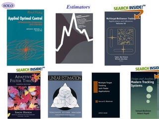
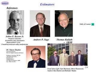

![216
SOLO Review of Probability
Normal (Gaussian) Distribution
Karl Friederich Gauss
1777-1855
( )
( )
σπ
σ
µ
σµ
2
2
exp
,;
2
2
−
−
=
x
xp
( ) ( )
∫
∞−
−
−=
x
du
u
xP 2
2
2
exp
2
1
,;
σ
µ
σπ
σµ
( ) µ=xE
( ) σ=xVar
( ) ( )[ ]
( ) ( )
−=
−
−=
=Φ
∫
∞+
∞−
2
exp
exp
2
exp
2
1
exp
22
2
2
σω
µω
ω
σ
µ
σπ
ωω
j
duuj
u
xjE
Probability Density Functions
Cumulative Distribution Function
Mean Value
Variance
Moment Generating Function](https://image.slidesharecdn.com/2-estimators-150110062422-conversion-gate02/85/2-estimators-215-320.jpg)
![217
SOLO Review of Probability
Moments
Normal Distribution ( ) ( ) ( )[ ]
σπ
σ
σ
2
2/exp
;
22
x
xpX
−
=
[ ] ( )
−⋅
=
oddnfor
evennforn
xE
n
n
0
131 σ
[ ]
( )
+=
=−⋅
= +
12!2
2
2131
12
knfork
knforn
xE kk
n
n
σ
π
σ
Proof:
Start from: and differentiate k time with respect to a( ) 0exp 2
>=−∫
∞
∞−
a
a
dxxa
π
Substitute a = 1/(2σ2
) to obtain E [xn
]
( ) ( ) 0
2
1231
exp 12
22
>
−⋅
=− +
∞
∞−
∫ a
a
k
dxxax kk
k π
[ ] ( ) ( )[ ] ( ) ( )[ ]
( ) ( ) 12
!
0
122/
0
222221212
!2
2
exp
2
22
2/exp
2
2
2/exp
2
1
2
+
∞+
=
∞∞
∞−
++
=−=
−=−=
∫
∫∫
kk
k
k
k
xy
kkk
kdyyy
xdxxxdxxxxE
σ
πσ
σ
π
σ
σπ
σ
σπ
σ
Now let compute:
[ ] [ ]( )2244
33 xExE == σ
Chi-square](https://image.slidesharecdn.com/2-estimators-150110062422-conversion-gate02/85/2-estimators-216-320.jpg)
![218
SOLO Review of Probability
Normal (Gaussian) Distribution (continue – 1)
Karl Friederich Gauss
1777-1855
( ) ( ) ( )
−−−= −−
xxPxxPPxxp
T 12/1
2
1
exp2,; π
A Vector – Valued Gaussian Random Variable has the
Probability Density Functions
where
{ }xEx
= Mean Value
( )( ){ }T
xxxxEP
−−= Covariance Matrix
If P is diagonal P = diag [σ1
2
σ2
2
… σk
2
] then the components of the random vector
are uncorrelated, and
x
( )
( ) ( ) ( ) ( )
∏=
−
−
−
−
=
−
−
−
−
−
−
=
−
−
−
−
−
−
−=
k
i i
i
ii
k
k
kk
kk
k
T
kk
xxxxxxxx
xx
xx
xx
xx
xx
xx
PPxxp
1
2
2
2
2
2
2
2
2
22
1
2
1
2
11
22
11
1
2
2
2
2
1
22
11
2/1
2
2
exp
2
2
exp
2
2
exp
2
2
exp
0
0
2
1
exp2,;
σπ
σ
σπ
σ
σπ
σ
σπ
σ
σ
σ
σ
π
therefore the
components of the
random vector are
also independent](https://image.slidesharecdn.com/2-estimators-150110062422-conversion-gate02/85/2-estimators-217-320.jpg)

![220
SOLO Review of Probability
Estimation of the Mean and Variance of a Random Variable (Unknown Statistics)
{ } { } jimxExE ji ,∀==
Define
Estimation of the
Population mean
∑=
=
k
i
ik x
k
m
1
1
:ˆ
A random variable, x, may take on any values in the range - ∞ to + ∞.
Based on a sample of k values, xi, i = 1,2,…,k, we wish to compute the sample mean, ,
and sample variance, , as estimates of the population mean, m, and variance, σ2
.
2
ˆkσ
kmˆ
( )
{ }
( ) ( ) ( )[ ] ( ) ( )[ ]
2
1
2
1
222
2
22222
1 11
2
1
2
2
11
2
1
2
11
1
1
1
1
1
21
11
2
1
ˆˆ2
1
ˆ
1
σσ
σσσ
k
k
kk
mkmkk
k
mmk
k
m
k
xx
k
Ex
k
xExE
k
mxmxE
k
mx
k
E
k
i
k
i
k
i
k
l
l
k
j
j
k
j
jii
k
k
i
ik
k
i
i
k
i
ki
−
=
−=
++−+++−−+=
+
−=
+−=
−
∑
∑
∑ ∑∑∑
∑∑∑
=
=
= ===
===
{ } { } jimxExE ji ,2222
∀+== σ
{ } { } mxE
k
mE
k
i
ik == ∑=1
1
ˆ
{ } { } { } jimxExExxE ji
tindependenxx
ji
ji
,2
,
∀==
Compute
Biased
Unbiased](https://image.slidesharecdn.com/2-estimators-150110062422-conversion-gate02/85/2-estimators-219-320.jpg)

![224
SOLO Review of Probability
Estimation of the Mean and Variance of a Random Variable (continue - 4)
Let Compute:
( ){ } ( ) ( )
( ) ( ) ( ) ( )[ ]
( ) ( ) ( ) ( )
−−
−
+−
−
−
+−
−
=
−−+−−+−
−
=
−−+−
−
=
−−
−
=−=
∑∑
∑
∑∑
==
=
==
2
22
11
2
2
2
1
22
2
2
1
2
2
2
1
22222
ˆ
ˆ
11
ˆ2
1
1
ˆˆ2
1
1
ˆ
1
1
ˆ
1
1
ˆ:2
σ
σ
σσσσσσ
k
k
i
i
k
k
i
i
k
i
kkii
k
i
ki
k
i
kik
mm
k
k
mx
k
mm
mx
k
E
mmmmmxmx
k
E
mmmx
k
Emx
k
EE
k
( )
( ){ } ( ){ } ( ){ } ( ){ }
( )
( ){ } ( )
( ){ }
( ){ }
( )
( ){ } ( ){ }
( )
( ){ } ( )
( ){ }
( ){ }
( )
( ){ } ( ){ }
( )
( ){ }
( )
( ){ }
k
k
k
i
i
k
k
i
i
k
k
k
i
i
k
k
i
i
k
k
k
i
i
k
k
k
k
i
i
k
k
k
i
k
ij
j
ji
k
k
i
i
mmE
k
k
mxE
k
mmE
mxE
k
mmEk
mxE
k
mxE
k
mmEk
mxE
k
mmE
mmE
k
k
mxE
k
mmE
mxEmxEmxE
kk
/
2
2
1
0
2
0
1
0
2
3
1
2
2
1
2
2
/
2
1
3
2
0
44
2
2
1
2
2
/
2
1 1
22
1
4
2
2
ˆ
2
222
22
22
4
2
ˆ
1
2
1
ˆ4
1
ˆ4
1
2
1
ˆ2
1
ˆ4
ˆ
11
ˆ4
1
1
σ
σσσ
σσ
σσ
µ
σ
σσ
σ
σσ
−
−
−−
−
−
−−
−
−
+
−
−
−−
−
−
+−
−
−
+
+−
−
+−
−
−
+
−−+−
−
≈
∑∑
∑∑∑
∑∑ ∑∑
==
===
==
≠
==
Since (xi – m), (xj - m) and are all independent for i ≠ j:( )kmm ˆ−](https://image.slidesharecdn.com/2-estimators-150110062422-conversion-gate02/85/2-estimators-223-320.jpg)
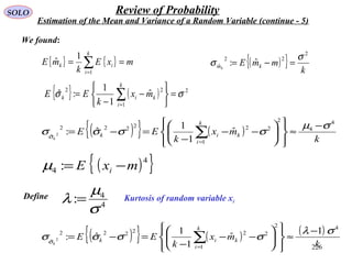
![227
SOLO Review of Probability
Estimation of the Mean and Variance of a Random Variable (continue - 6)
[ ] ϕσσσ σσ =≤≤
2
ˆ
2
k
2
k
ˆ-0Prob n
For high values of k, according to the Central Limit Theorem the estimations of mean
and of variance are approximately gaussian random variables.
kmˆ
2
ˆkσ
We want to find a region around that
will contain σ2
with a predefined probability
φ as function of the number of iterations k.
2
ˆkσ
Since are approximately gaussian random
variables nσ is given by solving:
2
ˆkσ
ϕζζ
π
σ
σ
=
−∫
+
−
n
n
d2
2
1
exp
2
1 nσ φ
1.000 0.6827
1.645 0.9000
1.960 0.9500
2.576 0.9900
Cumulative Probability within nσ
Standard Deviation of the Mean for a
Gaussian Random Variable
22
k
22 1
ˆ-
1
σ
λ
σσσ
λ
σσ
k
n
k
n
−
≤≤
−
−
22
k
2
1
1
ˆ-1
1
σ
λ
σσ
λ
σσ
−
−
≤≤
+
−
−
k
n
k
n](https://image.slidesharecdn.com/2-estimators-150110062422-conversion-gate02/85/2-estimators-226-320.jpg)
![228
SOLO Review of Probability
Estimation of the Mean and Variance of a Random Variable (continue - 7)
[ ] ϕσσσ σσ =≤≤
2
ˆ
2
k
2
k
ˆ-0Prob n
22
k
22 1
ˆ-
1
σ
λ
σσσ
λ
σσ
k
n
k
n
−
≤≤
−
−
22
k
2
1
1
ˆ-1
1
σ
λ
σσ
λ
σσ
−
−
≤≤
+
−
−
k
n
k
n
22
ˆ
1
2
k
σ
λ
σσ
k
−
=
22
k
2 1
1ˆ
1
1 σ
λ
σσ
λ
σσ
−
−≥≥
−
+
k
n
k
n
−
−
≥≥
−
+
k
n
k
n
1
1
ˆ
1
1
2
2
k
2
λ
σ
σ
λ
σ
σσ
k
n
k
n
1
1
:ˆ:
1
1
k
−
−
=≥≥=
−
+
λ
σ
σσσ
λ
σ
σσ](https://image.slidesharecdn.com/2-estimators-150110062422-conversion-gate02/85/2-estimators-227-320.jpg)


![231
SOLO Review of Probability
Estimation of the Mean and Variance of a Random Variable (continue - 10)
k
n
k
n
kk 1ˆ
1
:&
1ˆ
1
:
00
−
−
=
−
+
=
λ
σ
σ
λ
σ
σ
σσ
Monte-Carlo Procedure
Choose the Confidence Level φ and find the corresponding nσ
using the normal (gaussian) distribution.
nσ φ
1.000 0.6827
1.645 0.9000
1.960 0.9500
2.576 0.9900
1
Run a few sample k0 > 20 and estimate λ according to2
( )
( )
2
1
2
0
1
4
0
0
0
0
0
0
ˆ
1
ˆ
1
:ˆ
−
−
=
∑
∑
=
=
k
i
ki
k
i
ki
k
mx
k
mx
k
λ∑=
=
0
0
10
1
:ˆ
k
i
ik x
k
m
3 Compute and as function of kσ σ
4 Find k for which
[ ] ϕσσσ σσ =≤≤
2
ˆ
2
k
2
k
ˆ-0Prob n
5 Run k-k0 simulations](https://image.slidesharecdn.com/2-estimators-150110062422-conversion-gate02/85/2-estimators-230-320.jpg)
![233
SOLO Review of Probability
Estimation of the Mean and Variance of a Random Variable (continue - 12)
Kurtosis of random variable xi
Kurtosis
Kurtosis (from the Greek word κυρτός, kyrtos or kurtos, meaning bulging) is a measure
of the "peakedness" of the probability distribution of a real-valued random variable.
Higher kurtosis means more of the variance is due to infrequent extreme deviations, as
opposed to frequent modestly-sized deviations.
1905 Pearson defines Kurtosis,
as a measure of departure from normality in a paper published in
Biometrika. λ=3 for the normal distribution and the terms
‘leptokurtic’ (λ>3), mesokurtic (λ=3), platikurtic (λ<3) are
introduced.
( ){ } ( ){ }[ ]224
/: mxEmxE ii −−=λ
( ){ }
( ){ }[ ]22
4
:
mxE
mxE
i
i
−
−
=λ
Karl Pearson
(1857 –1936)
A leptokurtic distribution has a more acute "peak" around the mean (that is,
a higher probability than a normally distributed variable of values near the
mean) and "fat tails" (that is, a higher probability than a normally distributed
variable of extreme values).
A platykurtic distribution has a smaller "peak" around the mean (that is, a lower
probability than a normally distributed variable of values near the mean) and
"thin tails" (that is, a lower probability than a normally distributed variable of
extreme values).](https://image.slidesharecdn.com/2-estimators-150110062422-conversion-gate02/85/2-estimators-232-320.jpg)
![235
SOLO Review of Probability
Estimation of the Mean and Variance of a Random Variable (continue - 14)
Skewness of random variable xi
Skewness
( ){ }
( ){ }[ ] 2/32
3
:
mxE
mxE
i
i
−
−
=γ Karl Pearson
(1857 –1936)
Negative skew: The left tail is longer; the mass of the distribution is concentrated on
the right of the figure. The distribution is said to be left-skewed.
1
Positive skew: The right tail is longer; the mass of the distribution is concentrated
on the left of the figure. The distribution is said to be right-skewed.
2
More data in the left tail than
it would be expected in a
normal distribution
More data in the righttail than
it would be expected in a
normal distribution
Karl Pearson suggested two simpler calculations as a measure of skewness:
• (mean - mode) / standard deviation
• 3 (mean - median) / standard deviation](https://image.slidesharecdn.com/2-estimators-150110062422-conversion-gate02/85/2-estimators-234-320.jpg)
![239
SOLO Review of Probability
Estimate the value of a constant x, given discrete measurements of x corrupted by an
uncorrelated gaussian noise sequence with zero mean and variance r0.
The scalar equations describing this situation are:
kk xx =+1
kkk vxz +=
System
Measurement ( )0,0~ rNvk
The Discrete Kalman Filter is given by:
( ) ( )+=−+ kk xx ˆˆ 1
( ) ( ) ( ) ( )[ ] ( )[ ]−−+−−+−=+ ++
−
++++
+
11
1
01111
ˆˆˆ
1
kk
K
kkkk xzrppxx
k
0
1 kkk
I
kk wxx Γ+Φ=+
kk
I
kk vxHz +=
( ) ( )[ ] ( )[ ]{ }
( )
( )+=ΓΓ+Φ+Φ=−−−−=− +++++ k
T
I
T
kk
I
k
T
kkkkk pQpxxxxEp
0
11111
ˆˆ
( ) ( )[ ] ( )[ ]{ }
( ) ( )
( )
( )
( ) ( ) ( )
( ) 0
0
11
1
0111111
11111
1
1
ˆˆ
rp
pr
pHrHpHHpp
xxxxEp
k
k
pp
k
I
k
K
T
I
kk
I
k
T
I
kkk
T
kkkkk
kk
k
++
+
=−
+−−−−=
−+−+=+
+=−
++
−
++++++
+++++
+
+
General Form
with Known Statistics Moments Using a Discrete Recursive Filter
Estimation of the Mean and Variance of a Random Variable](https://image.slidesharecdn.com/2-estimators-150110062422-conversion-gate02/85/2-estimators-238-320.jpg)
![240
SOLO Review of Probability
Estimate the value of a constant x, given discrete measurements of x corrupted by an
uncorrelated gaussian noise sequence with zero mean and variance r0.
We found that the Discrete Kalman Filter is given by:
( ) ( ) ( )[ ]+−++=+ +++ kkkkk xzKxx ˆˆˆ 111
( ) ( )
( )
( )
( )
0
0
0
1
1
r
p
p
rp
pr
p
k
k
k
k
k
+
+
+
=
++
+
=++
( )
0
0
0
1
1
r
p
p
p
+
=+ ( ) ( )
( )
0
1
1
2
1
r
p
p
p
+
+
+
=+ ( )
k
r
p
p
pk
0
0
0
1+
=+
( )
( ) 0
1
rp
p
K
k
k
k
++
+
=+
( )
( ) 0
1
rp
p
K
k
k
k
++
+
=+( ) ( )
( )
( )[ ]+−
++
++=+ ++ kkkk xz
k
r
p
r
p
xx ˆ
11
ˆˆ 1
0
0
0
0
1
0=k
1=k
0
0
0
2
1
r
p
p
+
=
( )11
1
1
0
0
0
0
0
0
0
0
0
0
0
++
=
+
+
+
=
k
r
p
r
p
r
k
r
p
p
k
r
p
p
with Known Statistics Moments Using a Discrete Recursive Filter (continue – 1)
Estimation of the Mean and Variance of a Random Variable](https://image.slidesharecdn.com/2-estimators-150110062422-conversion-gate02/85/2-estimators-239-320.jpg)
![241
SOLO Review of Probability
Estimate the value of a constant x, given continuous measurements of x corrupted by an
uncorrelated gaussian noise sequence with zero mean and variance r0.
The scalar equations describing this situation are:
0=x
vxz +=
System
Measurement ( )rNv ,0~
The Continuous Kalman Filter is given by:
( ) ( ) ( ) ( ) ( )[ ] ( ) 00ˆ&ˆˆˆ
1
1
0
=−
+=
+
−
xtxtzrHtptxAtx
kK
I
00
wxAx Γ+=
vxHz
I
+=
( ) ( ) ( )[ ] ( ) ( )[ ]{ }T
txtxtxtxEtp −−= ˆˆ:
( ) ( ) ( ) ( ) ( ) ( ) ( ) ( ) ( ) ( ) ( ) ( ) 12
1
1
000
−−
−=−++= rtptptHrtHtptGQtGtAtptptAtp TT
I
TT
General Form
with Known Statistics Moments Using a Continuous Recursive Filter
Estimation of the Mean and Variance of a Random Variable
( ) ( ) ( ) 0
12
0& ptprtptp ==−= −
or:
∫∫ −=
tp
p
dt
rp
pd
0
2
0
1 ( )
t
r
p
p
tp
0
0
1+
=
( )
t
r
p
r
p
rtpK
0
0
1
1+
== −
( ) ( )[ ]txz
t
r
p
r
p
tx ˆ
1
ˆ
0
0
−
+
=](https://image.slidesharecdn.com/2-estimators-150110062422-conversion-gate02/85/2-estimators-240-320.jpg)
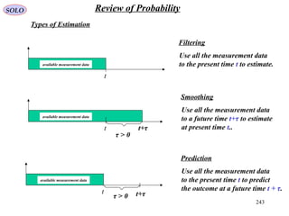
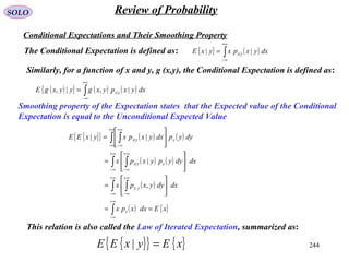
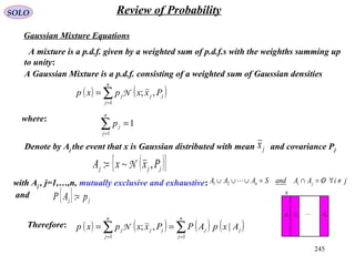
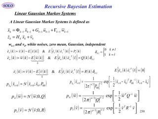
![251
Recursive Bayesian EstimationSOLO
Linear Gaussian Markov Systems (continue – 2)
111111 −−−−−− Γ++Φ= kkkkkkk wuGxx
Prediction phase (before zk measurement)
{ } { } { }
0
1:111111:1111:11| |||:ˆ −−−−−−−−−− Γ++Φ== kkkkkkkkkkkk ZwEuGZxEZxEx
or 111|111|
ˆˆ −−−−−− +Φ= kkkkkkk uGxx
The expectation is
{ }[ ] { }[ ]{ }
( )[ ] ( )[ ]{ }1:1111|111111|111
1:11|1|1|
|ˆˆ
|ˆˆ:
−−−−−−−−−−−−−
−−−−
Γ+−ΦΓ+−Φ=
−−=
k
T
kkkkkkkkkkkk
k
T
kkkkkkkk
ZwxxwxxE
ZxExxExEP
( ) ( ){ } ( ){ }
( ){ } { } T
k
Q
T
kkk
T
k
T
kkkkk
T
k
T
kkkkk
T
k
P
T
kkkkkkk
wwExxwE
wxxExxxxE
kk
11111
0
1|1111
1
0
11|11111|111|111
ˆ
ˆˆˆ
1|1
−−−−−−−−−−
−−−−−−−−−−−−−−
ΓΓ+Φ−Γ+
Γ−Φ+Φ−−Φ=
−−
T
kk
T
kkkkkk QPP 1111|111| −−−−−−− ΓΓ+ΦΦ=
{ } ( )1|1|1:1 ,ˆ;| −−− = kkkkkkk PxxZxP N
Since is a Linear Combination of Independent
Gaussian Random Variables:
111111 −−−−−− Γ++Φ= kkkkkkk wuGxx
Table of Content](https://image.slidesharecdn.com/2-estimators-150110062422-conversion-gate02/85/2-estimators-250-320.jpg)
![252
Random VariablesSOLO
Random Variable:
A variable x determined by the outcome Ω of a random experiment.
( )Ω= xx
Random Process or Stochastic Process:
A function of time x determined by the outcome Ω of a random experiment.
( ) ( )Ω= ,txtx
1
Ω
2
Ω
3Ω
4Ω
x
t
This is a family or an ensemble of
functions of time, in general different
for each outcome Ω.
Mean or Ensemble Average of the Random Process: ( ) ( )[ ] ( ) ( )∫
+∞
∞−
=Ω= ξξξ dptxEtx tx
,:
Autocorrelation of the Random Process: ( ) ( ) ( )[ ] ( ) ( ) ( )∫ ∫
+∞
∞−
+∞
∞−
=ΩΩ= ηξξξη ddptxtxEttR txtx 21 ,2121
,,:,
Autocovariance of the Random Process: ( ) ( ) ( )[ ] ( ) ( )[ ]{ }221121 ,,:, txtxtxtxEttC −Ω−Ω=
( ) ( ) ( )[ ] ( ) ( ) ( ) ( ) ( )2121212121 ,,,, txtxttRtxtxtxtxEttC −=−ΩΩ=](https://image.slidesharecdn.com/2-estimators-150110062422-conversion-gate02/85/2-estimators-251-320.jpg)
![253
Random VariablesSOLO
Stationarity of a Random Process
1. Wide Sense Stationarity of a Random Process:
• Mean Average of the Random Process is time invariant:
( ) ( )[ ] ( ) ( ) .,: constxdptxEtx tx
===Ω= ∫
+∞
∞−
ξξξ
• Autocorrelation of the Random Process is of the form: ( ) ( ) ( )τ
τ
RttRttR
tt 21:
2121
,
−=
=−=
( ) ( ) ( )[ ] ( ) ( ) ( ) ( )12,2121 ,,,:, 21
ttRddptxtxEttR txtx === ∫ ∫
+∞
∞−
+∞
∞−
ηξξξηωωsince:
We have: ( ) ( )ττ −= RR
Power Spectrum or Power Spectral Density of a Stationary Random Process:
( ) ( ) ( )∫
+∞
∞−
−= ττωτω djRS exp:
2. Strict Sense Stationarity of a Random Process:
All probability density functions are time invariant: ( ) ( ) ( ) .,,
constptp xtx
== ωωω
Ergodicity:
( ) ( ) ( )[ ]Ω==Ω=Ω ∫
+
−∞→
,,
2
1
:, lim txExdttx
T
tx
Ergodicity
T
TT
A Stationary Random Process for which Time Average = Assembly Average](https://image.slidesharecdn.com/2-estimators-150110062422-conversion-gate02/85/2-estimators-252-320.jpg)
![254
Random VariablesSOLO
Time Autocorrelation:
Ergodicity:
( ) ( ) ( ) ( ) ( )∫
+
−∞→
Ω+Ω=Ω+Ω=
T
TT
dttxtx
T
txtxR ,,
2
1
:,, lim τττ
For a Ergodic Random Process define
Finite Signal Energy Assumption: ( ) ( ) ( ) ∞<Ω=Ω= ∫
+
−∞→
T
TT
dttx
T
txR ,
2
1
,0 22
lim
Define: ( )
( )
≤≤−Ω
=Ω
otherwise
TtTtx
txT
0
,
:, ( ) ( ) ( )∫
+∞
∞−
Ω+Ω= dttxtx
T
R TTT
,,
2
1
: ττ
( ) ( ) ( ) ( ) ( ) ( ) ( )
( ) ( ) ( ) ( ) ( ) ( )∫∫∫
∫∫∫
−−
−
−
+∞
−
−
−
−
∞−
Ω+Ω−Ω+Ω=Ω+Ω=
Ω+Ω+Ω+Ω++Ω=
T
T
TT
T
T
TT
T
T
TT
T
TT
T
T
TT
T
TTT
dttxtx
T
dttxtx
T
dttxtx
T
dttxtx
T
dttxtx
T
dttxtx
T
R
τ
τ
τ
τ
τττ
ττωττ
,,
2
1
,,
2
1
,,
2
1
,,
2
1
,,
2
1
,,
2
1
00
Let compute:
( ) ( ) ( ) ( ) ( )∫∫ −∞→−∞→∞→
Ω+Ω−Ω+Ω=
T
T
TT
T
T
T
TT
T
T
T
dttxtx
T
dttxtx
T
R
τ
τττ ,,
2
1
,,
2
1
limlimlim
( ) ( ) ( )ττ Rdttxtx
T
T
T
TT
T
=Ω+Ω∫−∞→
,,
2
1
lim
( ) ( ) ( ) ( )[ ] 0,,
2
1
,,
2
1
suplimlim →
Ω+Ω≤Ω+Ω
≤≤−∞→−∞→
∫ τττ
ττ
txtx
T
dttxtx
T
TT
TtTT
T
T
TT
T
therefore: ( ) ( )ττ RRT
T
=
→∞
lim
( ) ( ) ( )[ ]Ω==Ω=Ω ∫
+
−∞→
,,
2
1
:, lim txExdttx
T
tx
Ergodicity
T
TT
T− T+
( )txT
t](https://image.slidesharecdn.com/2-estimators-150110062422-conversion-gate02/85/2-estimators-253-320.jpg)
![255
Random VariablesSOLO
Ergodicity (continue - 1):
( ) ( ) ( ) ( ) ( )
( ) ( )[ ] ( ) ( )( )[ ]
( ) ( ) ( ) ( )( )
( ) ( ) ( ) ( ) [ ]TTTT
TT
TT
TTT
XX
T
dvvjvxdttjtx
T
dtjtxdttjtx
T
ddttjtxtjtx
T
dttxtxdj
T
djR
*
2
1
exp,exp,
2
1
exp,exp,
2
1
exp,exp,
2
1
,,exp
2
1
exp
=−ΩΩ=
+−Ω+Ω=
+−Ω+Ω=
Ω+Ω−=−
∫∫
∫∫
∫ ∫
∫ ∫∫
∞+
∞−
∞+
∞−
∞+
∞−
∞+
∞−
∞+
∞−
∞+
∞−
+∞
∞−
+∞
∞−
+∞
∞−
ωω
ττωτω
ττωτω
τττωττωτLet compute:
where: and * means complex-conjugate.( ) ( )∫
+∞
∞−
−Ω= dvvjvxX TT ωexp,:
Define:
( ) ( ) ( ) ( ) ( ) ( )[ ]∫ ∫∫
+∞
∞−
+
−∞→
+∞
∞−∞→∞→
Ω+Ω−=
−=
= τττωττωτω ddttxtxE
T
jdjRE
T
XX
ES
T
T
TT
T
T
T
TT
T
,,
2
1
expexp
2
: limlimlim
*
Since the Random Process is Ergodic we can use the Wide Stationarity Assumption:
( ) ( )[ ] ( )ττ RtxtxE TT =Ω+Ω ,,
( ) ( ) ( ) ( ) ( )
( ) ( )∫
∫ ∫∫ ∫
∞+
∞−
+∞
∞−
+
−∞→
+∞
∞−
+
−∞→∞→
−=
−=
−=
=
ττωτ
ττωττττωω
djR
ddt
T
jRddtR
T
j
T
XX
ES
T
TT
T
TT
TT
T
exp
2
1
exp
2
1
exp
2
:
1
*
limlimlim
](https://image.slidesharecdn.com/2-estimators-150110062422-conversion-gate02/85/2-estimators-254-320.jpg)
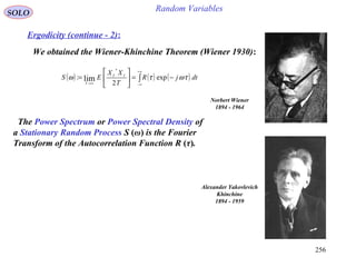
![257
Random VariablesSOLO
White Noise
A (not necessary stationary) Random Process whose Autocorrelation is zero for
any two different times is called white noise in the wide sense.
( ) ( ) ( )[ ] ( ) ( )211
2
2121
,,, ttttxtxEttR −=ΩΩ= δσ
( )1
2
tσ - instantaneous variance
Wide Sense Whiteness
Strict Sense Whiteness
A (not necessary stationary) Random Process in which the outcome for any two
different times is independent is called white noise in the strict sense.
( ) ( ) ( ) ( )2121,
,,21
ttttp txtx
−=Ω δ
A Stationary White Noise Random has the Autocorrelation:
( ) ( ) ( )[ ] ( )τδσττ 2
,, =Ω+Ω= txtxER
Note
In general whiteness requires Strict Sense Whiteness. In practice we have only
moments (typically up to second order) and thus only Wide Sense Whiteness.](https://image.slidesharecdn.com/2-estimators-150110062422-conversion-gate02/85/2-estimators-256-320.jpg)
![258
Random VariablesSOLO
White Noise
A Stationary White Noise Random has the Autocorrelation:
( ) ( ) ( )[ ] ( )τδσττ 2
,, =Ω+Ω= txtxER
The Power Spectral Density is given by performing the Fourier Transform of the
Autocorrelation:
( ) ( ) ( ) ( ) ( ) 22
expexp στωτδστωτω =−=−= ∫∫
+∞
∞−
+∞
∞−
dtjdtjRS
( )ωS
ω
2
σ
We can see that the Power Spectrum Density contains all frequencies at the same
amplitude. This is the reason that is called White Noise.
The Power of the Noise is defined as: ( ) ( ) 2
0 σωτ ==== ∫
+∞
∞−
SdtRP](https://image.slidesharecdn.com/2-estimators-150110062422-conversion-gate02/85/2-estimators-257-320.jpg)
![261
Random VariablesSOLO
Table of Content
Markov Processes
Examples of Markov Processes:
3. Continuous Linear Dynamic System
( ) ( ) ( )
( ) ( )txCtz
tvtxAtx
=
+=
The Autocorrelation of the output is:
( ) ( ) ( )∫
+∞
∞−
= ξξξ dvtHtz ,
( ) ( ) ( )[ ] ( ) ( ) ( ) ( )
( ) ( ) ( )[ ] ( ) ( ) ( ) ( )
( ) ( ) ( ) ( )∫∫
∫ ∫∫ ∫
∫∫
∞+
∞−
−=∞+
∞−
∞+
∞−
∞+
∞−
∞+
∞−
∞+
∞−
+∞
∞−
+∞
∞−
+=−+−=
−−+−=−+−=
−+−=+=
ζτζζξξτξ
ξξξξδξτξξξξτξξξ
ξξτξξξξττ
ξζ
dHSHdtHStH
ddtHStHddtHvvEtH
dtHvdvtHEtztzER
T
vv
t
T
vv
T
vv
TT
TTT
zz
1
111
212121211211
222111
( ) ( ) ( )[ ] ( )τδττ vv
T
vv StvtvER =+=
( ) ( ) ( ) ( ) ( ) vvvvvvvv SdjSdjRS =−=−= ∫∫
+∞
∞−
+∞
∞−
ττωτδττωτω expexp
( ) ( ) ( )
( ) ( )
( ) ( ) ( )
( ) ( ) ( ) ( )( ) ( ) ( ) ( ) ( )
( ) ( ) ( ) ( ) ( ) ( )ωωχχωχζζωζ
χχωζζωζχττζωζζωζτζ
ττωζτζζττωτω
χτζ
ττ
*
expexp
expexpexpexp
expexp
HH vv
T
vv
T
vv
T
vv
T
vv
RR
zzzz
SdjHSdjH
djdjHSHdjdjHSH
djdHSHdjRS
zzzz
=
−=
−=−−−=
−−=−=
∫∫
∫ ∫∫ ∫
∫ ∫∫
∞+
∞−
∞+
∞−
∞+
∞−
∞+
∞−
=+∞+
∞−
∞+
∞−
+∞
∞−
+∞
∞−
−=+∞
∞−
( ) ( ) ( ) ( ) conjugatecomplexSS vvzz −== ∗
ωωωω *
HH](https://image.slidesharecdn.com/2-estimators-150110062422-conversion-gate02/85/2-estimators-260-320.jpg)
![262
Random VariablesSOLO
Table of Content
Markov Processes
Examples of Markov Processes:
4. Continuous Linear Dynamic System ( ) ( ) ( )∫
+∞
∞−
= ξξξ dvthtz ,
( ) ( ) ( )[ ] ( )τδσττ
2
vvv tvtvER =+= ( ) 2
vvvS σω =
v (t) z (t)
( )
xj
K
H
ωω
ω
/1+
=
( )
x
j
K
H
ωω
ω
/1+
=
The Power Spectral Density of the output is:
( ) ( ) ( ) ( )
( )2
22
*
/1 x
v
vvzz
K
HSHS
ωω
σ
ωωωω
+
==
( )
( )2
22
/1 x
vv
zz
K
S
ωω
σ
ω
+
=
ω
x
ω
22
vv
K σ
2/
22
vv
K σ
The Autocorrelation of the output is:
( ) ( ) ( )
( )
( )
( )
( )∫∫
∫
∞+
∞−
=
∞+
∞−
+∞
∞−
−
−
=
+
=
=
dss
s
K
j
dj
K
djSR
x
v
js
x
v
zzzz
τ
ω
σ
π
ωτω
ωω
σ
π
ωτωω
π
τ
ω
exp
/12
1
exp
/12
1
exp
2
1
2
22
2
22
ωj
xω
R
( )
0
/1
2
22
=
−∫∞→R
s
x
vv
dse
s
K τ
ω
σ
( )
0
/1
2
22
=
−∫∞→R
s
x
vv
dse
s
K τ
ω
σ
xω−
σ
ωσ js +=
0<τ
0>τ
( ) τωσω
ω x
e
K
R vvx
zz
=
=
2
22
τ
2/
22
vvxK σω
( )τω
σω
x
vx
K
−= exp
2
22
( )
( )
( )
( )
>
+
−
−=
−
−
<
−
−
=
−
−
=
∫
∫
→
−→
0
exp
Reexp
2
1
0
exp
Reexp
2
1
222
22
222
222
22
222
τ
ω
τσω
τ
ω
σω
π
τ
ω
τσω
τ
ω
σω
π
ωω
ωω
x
vx
x
vx
x
vx
x
vx
s
sK
sdss
s
K
j
s
sK
sdss
s
K
j
x
x](https://image.slidesharecdn.com/2-estimators-150110062422-conversion-gate02/85/2-estimators-261-320.jpg)
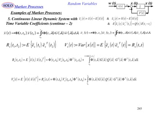
![267
Random VariablesSOLO Markov Processes
Examples of Markov Processes:
6. Discrete Linear Dynamic System with Variable Coefficients (continue – 1)
( ) ( ){ } ( ) ( ) ( ){ } ( ) ( ) ( ) ( ){ }∑
−+
=
Γ++Φ++Φ=+
1
1,,
lk
kn
T
xw
T
xx
T
xx keneEnnlkkekeEklkkelkeE
( ) ( ) ( ) ( ) ( ) ( )∑
−+
=
Γ++Φ++Φ=+
1
1,,
lk
kn
wxx nennlkkeklklke
( ) ( ) ( ) ( ) ( ) ( )∑
−
−=
Γ+Φ+−−Φ=
1
1,,
k
lkm
wxx memmklkelkkke
=
−
→
,2,1l
lk
k
( ) ( ){ } ( ) ( ){ } ( ) ( ) ( ){ }
( )
( ) ( )∑
−
−=
−
+ΦΓ+−Φ−=
1
1,,
k
lkm
TT
mnQ
T
ww
TT
xw
T
xw mkmmeneElkklkeneEkeneE
w
δ
[ ]
[ ]
=
−−∈
−+∈
,2,1
1,
1,
l
klkm
lkkn
( ) ( ){ }
( ) 0
0
=−
=−
nmQ
lkeneE
w
T
xw
δ
( ) ( ){ } 0=keneE
T
xw
( ) ( ){ } ( ) ( ) ( ){ }kekeEklkkelkeE
T
xx
T
xx ,+Φ=+](https://image.slidesharecdn.com/2-estimators-150110062422-conversion-gate02/85/2-estimators-266-320.jpg)
![268
Random VariablesSOLO Markov Processes
Examples of Markov Processes:
6. Discrete Linear Dynamic System with Variable Coefficients (continue – 2)
( ) ( ){ } ( ) ( ){ } ( ) ( ) ( ){ } ( ) ( )∑
−+
=
++ΦΓ++Φ=+
1
1,,
lk
kn
TTT
wx
TT
xx
T
xx nlknnekeEklkkekeElkekeE
( ) ( ) ( ) ( ) ( ) ( )∑
−+
=
Γ++Φ++Φ=+
1
1,,
lk
kn
wxx nennlkkeklklke
( ) ( ) ( ) ( ) ( ) ( )∑
−
−=
Γ+Φ+−−Φ=
1
1,,
k
lkm
wxx memmklkelkkke
=
−
→
,2,1l
lk
k
( ) ( ){ } ( ) ( ) ( ){ } ( ) ( ) ( ) ( ){ }
( )
∑
−
−=
−
Γ+Φ+−−Φ=
1
1,,
k
lkm
nmQ
T
ww
T
w
T
x
T
wx
w
nemeEmmknelkeElkknekeE
δ
[ ]
[ ]
=
−−∈
−+∈
,2,1
1,
1,
l
klkm
lkkn
( ) ( ){ }
( ) 0
0
=−
=−
mnQ
nelkeE
w
T
wx
δ
( ) ( ){ } 0=nekeE
T
wx
( ) ( ){ } ( ) ( ){ } ( )klkkekeElkekeE TT
xx
T
xx ,+Φ=+
Table of Content](https://image.slidesharecdn.com/2-estimators-150110062422-conversion-gate02/85/2-estimators-267-320.jpg)
![272
SOLO Matrices
Trace of a Square Matrix
The trace of a square matrix is defined as ( ) ( )T
nn
n
i
iinn AtraceaAtrace ×
=
× == ∑1
:
Proof:
q.e.d.
5
( ) ( ) ( )
A
Atrace
I
A
Atrace T
n
∂
∂
==
∂
∂ 1
( )
=
≠
==
∂
∂
=
∂
∂
∑= ji
ji
a
aA
Atrace
ij
n
i
ii
ijij
1
0
1
δ
6
( ) ( ) ( ) ( ) nmmnTTT
RBRCCBBC
A
BCAtrace
A
ABCtrace ××
∈∈==
∂
∂
=
∂
∂ 1
Proof:
( ) ( ) ( )[ ]ij
T
ji
m
p
pijp
ik
jl
n
l
m
p
n
k
klpklp
ijij
BCBCbcabc
aA
ABCtrace
===
∂
∂
=
∂
∂
∑∑∑∑ =
=
=
= = = 11 1 1
q.e.d.
7 If A, B, C ∈ Rnxn
,i.e. square matrices, then
( ) ( ) ( ) ( ) ( ) ( ) TTT
CBBC
A
BCAtrace
A
CABtrace
A
ABCtrace
==
∂
∂
=
∂
∂
=
∂
∂ 11](https://image.slidesharecdn.com/2-estimators-150110062422-conversion-gate02/85/2-estimators-271-320.jpg)
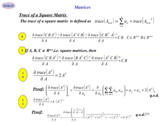
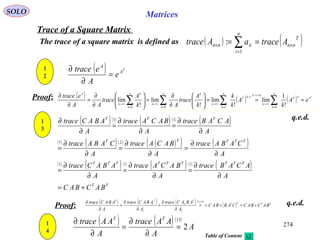
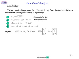
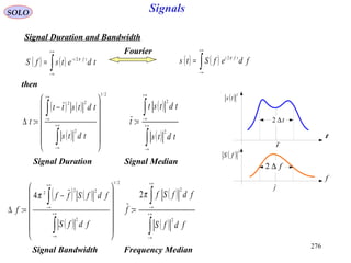

The document provides a comprehensive overview of various estimation techniques in control systems, specifically focusing on different types of Kalman filters and their applications. It details the history and development of these methods, highlighting significant contributions by key figures such as Gauss and Kolmogorov. Additionally, it discusses properties of estimators and optimal parameter estimation processes in linear stationary systems.


![Sensor Fusion Study - Ch3. Least Square Estimation [강소라, Stella, Hayden]](https://cdn.slidesharecdn.com/ss_thumbnails/chapter3-200521130800-thumbnail.jpg?width=640&height=640&fit=bounds)


![Polymer [ बहुलक ] Chemistry Notes PDF - Irfanullah Mehar - JJ Sir Chemistry.pdf](https://cdn.slidesharecdn.com/ss_thumbnails/polymerchemistrynotespdf-irfanullahmehar-jjsirchemistry-260210172118-3f9b37f7-thumbnail.jpg?width=640&height=640&fit=bounds)


