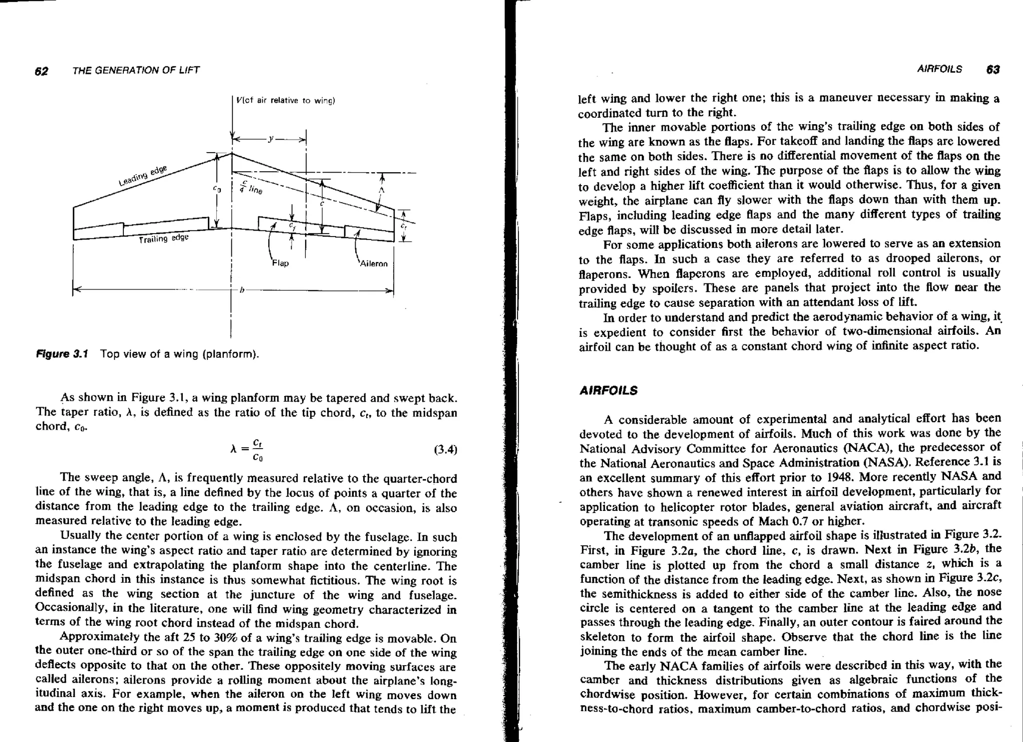
CONTENTS 
ONE INTRODUCTION 
A Brief History 
A Brief Introduction to the Technology of Aeronautics 
TWO FLUID MECHANICS 
Fluid Statics and the Atmosphere 
Fluid Dynamics 
Conservation of Mass 
The Momentum Theorem 
Euler's Equation of Motion 
Bernoulli's Equation 
Determination of Free-Stream Velocity 
Determination of True Airspeed 
Potential Flow 
Velocity Potential and Stream Function 
Elementary Flow Functions 
Vortex 
Source 
Biot-Savart Law 
The Calcuiation of Flows for Well-Defined Body Shapes 
The Circular Cylinder 
The Numerical Calculation of Potential Flow Around Arbitrary Bdy 
Shapes 
THREE THE GENERATION OF LIFT 
Wing Geometry 
Airfoils 
Airfoil Families 
N ACA Four-Digit Series 
NACA Five-Digit Series 
NACA 1-Series (Series 16) 
NACA 6-Series 
Modern AirfoiI Developments 
Prediction of AirfoiI Behavior 
Maximum Lift 
Flaps 
Plain Flaps 
SpIit Flaps 
Slotted Flaps
CONTENTS 
ONE INTRODUCT/ON 
A Brief History 
A Brief Introduction to the Technology of Aeronautics 
TWO FLUID MECHANICS 
Fluid Statics and the Atmosphere 
Fluid Dynamics 
Conservation of Mass 
The Momentum Theorem 
Euler's Equation of Motion 
Bernoulli's Equation 
Determination of Free-Stream Velocity 
Determination of True Airspeed 
Potential FIow 
Velocity Potential and Stream Function 
Elementary Flow Functions 
Vortex 
Source 
Biot-Savart Law 
The Calculation of Flows for Well-Defined Body Shapes 
The Circular Cylinder 
The Numerical Calculation of Potential Flow Around Arbitrary Body 
Shapes 
THREE THE GENERATION OF LIFT 
Wing Geometry 
Airfoils 
Airfoil Families 
NACA Four-Digit Series 
NACA Five-Digit Series 
NAC A 1-Series (Series 16) 
NACA &Series 
Modern Airfoil Developments 
Prediction of Airfoil Behavior 
Maximum Lift 
Flaps 
Plain Flaps 
SpIit Flaps 
Slotted Flaps
Flap Effectiveness ~n the Linear Range 
Leading Edge Devices 
The Optimum Airfoil for High Lift 
Powered-Lift Systems 
The Lifting Characteristics of a Finite Wing 
The Vortex System for a Wing 
The Maximum Lift of a Finite Wing 
Effect of Fuselage on CL,, 
Effect of Trim on 
Estimation of C,,,, for a Complete Airplane Configuration 
Airfoil Characteristics at Low Reynolds Numbers 
FOUR DRAG 
Skin Friction Drag 
Form Drag 
Drag of Streamlined Shapes 
Interference Drag 
Induced Drag 
Calculation of Induced Drag 
Effective Aspect Ratio 
Drag Breakdown and Equivalent Flat-Plate Area 
Drag Counts 
Average Skin Friction Coefficients 
Example Estimates of Drag Breakdown 
Trim Drag 
Cooling Drag 
Drag Reduction 
Winglets 
Reduction of Skin Friction Drag 
Drag Cleanup 
Total Airplane Drag 
FIVE LIFT AND DRAG AT HIGH MACH NUMBERS 
Qualitative Behavior of Airfoils as a Function of Mach Number 
Subsonic Flow at High Mach Numbers 
Fundamentals of Gas Dynamics 
One-Dimensional Isentropic Flow 
Normal Shock Waves 
Oblique Shock Waves 
Expansion Waves 
Transonic Airfoils 
Supersonic Airfoils 
Linearized Compressible PoteniiaI Flow 
Subsonic Flow 
Supersonic Flow (Ackeret Theory) 
Three-Dimensional Wings 
Characteristics of Sweptback Wings 
Delta Wings 
CONTENTS 
Supersonic Wings 
Subsonic Leading Edges 
Supersonic Leading Edges 
Effect of Mach Number on the Zero Lift Drag of Two- and Three- 
Dimensional Shapes 
Area Rule for Transonic Flow 
SIX THE PRODUCTlON OF THRUST 
A Brief History of the Piston Engine 
Piston Engine Characteristics 
Supercharged Engines 
Propeller Analysis 
Momentum Theory 
Blade Element Theories 
Momentum-Blade Element Theory 
Vortex Theory 
Practical Use of Propeller Charts 
Approximate Useful Relationships for PropeHers 
Propeller Selection 
Design of a New Propeller 
A Brief History of the Turbojet 
Description of the Gas Turbine Engine 
Engine Ratings 
Flat Rating 
Some Considerations Relating to Gas Turbine Performance 
Qualitative Comparison of the Performance of Turbojet, Turbofan, and 
Turboprop Engines 
Specific Engine Characteristics and Performance 
Turbojet 
Turbofan 
Turboprop 
Installation Losses 
Trends in Aircraft Propulsion 
SEVEN AIRPLANE PERFORMANCE 
Takeoff 
Ground Roll 
Effect of Wind 
Airborne Distance 
Balanced Field Length 
Rate of Climb, Time to Climb, and Ceilings 
Generalized Power-Required Curve 
Time to Climb 
Range 
Maximum Endurance 
Descent 
Landing 
xiii
X~V CONTENTS 
Airborne Distance 
Gro~ndR oll 
Range Payload 
Operating Limitations 
Flight Envelope 
Maneuvering Envelope (V-n Diagram) 
Gust Load Factors 
Energy Methods for Optimal Trajectories 
The Art of Estimating and Scaling 
EIGHT STATIC STABILITY AND CONTROL 
Introduction 
Coordinate System-Forces, Moments, and Velocities 
Longitudinal Static Stability 
Stick-Fixed Stability 
Stick-Fixed Neutral Point and Static Margin 
CM,, and Aerodynamic Center Location for a Finite Wing 
Downwash Angle 
Longitudinal Control 
Control Position as a Function of Lift Coefficient 
All-Movable Tail 
Stabilizer-EIevator 
Stabilator 
Control Forces 
Gearing 
Stick Force for A Stabifator 
Stick Force for a HorizontaI Stabilizer-Elevator Combination 
Estimation of Aerodynamic Hinge Moments 
Example Calculation of Stick Force 
Stick-Free Longitudinal Static Stability 
Elevator-Stabilizer Configuration 
Stabilator Configuration 
Stick-Free Static Margin 
Steady Maneuvering 
Horizontal Stabilizer-Elevator Configuration: Elevator Angle per g 
Stabilator Angle per g 
Stick Force per g 
Stabilizer-Elevator Configuration 
Stabilator 
Effect of Fuselage and Nacelles 
Effects of Propulsion System 
Propellers 
Jets 
Ground Effect 
Lateral and Directional Static Stability and Control 
Directional Static Stability 
Directional Control 
Lateral Control 
Adverse Yaw 
Roll Control by the Use of Spoilers 
Aileron Reversal 
Steady Rolling Motion 
Coupling Effects 
Rolling Moment with Rudder 
Rolling Moment with Yaw Rate 
Yawing Moment with Roll Rate 
Rolling Moment with Sideslip Angle-Dihedral Effect 
CONTENTS xv 
NINE LONGITUDINAL DYNAMIC STABlLlTY AND CONTROL 
Equations of Motion 
Linearization of the Equations 
A Summary Look at the Stability Derivatives and Other Parameters 
Affecting Longitudinal Dynamic Motion 
X Derivatives and Parameters 
Z Derivatives and Parameters 
M Derivatives and Parameters 
Examination and Reduction of Equations of Longitudinal Motion 
Solution of nth-Order Linear Differential Equations with Constant 
Coefficients 
Mode Shapes 
Phugoid (Long-Period Mode) 
Short-Period Mode 
Solution of the 1,ongitudinal Equations of Motion Using an Analog 
Computer 
Longitudinal Flying Qualities 
Phugoid Mode 
Flight Path Stability 
Short Period Mode 
TEN LATERAL-D/RECT/ONAL DYNAMIC STABlLlTY AND 
CONTROL 
Equations of Motion 
Euler Angles 
Reduction of the Lateral-Directional Equations of Motion 
A Summary Look at the Stability Derivatives and Other Parameters 
Affecting Lateral-DirectionaI Dy narnic Motion 
Y Derivatives 
Cy, c, 
CY, 
Cyar
xvi CONTENTS 
Cii 
Cl, 
N Derivatives 
C,,', 
c,, 
Chmi 
Ch'8" 
Lateral-Directional Equations for the Cherokee i80 
Mode Shapes 
Roll Mode 
Spiral Mode 
Oscillatory or "Dutch Roll" Mode 
Lateral Directional Flying Qualities 
Roll Mode 
Dutch Roll Mode 
Spiral Stability 
Spinning 
APPENDlX A.1 THE Sf SYSTEM 
APPENDIX A.2 STANDARD ATMOSPHERE 
APPENDIX A.3 AIRPLANE DATA 
APPENDIX A.4 NOMENCLATURE AND ABBREVlATlONS 
INDEX 
AERODYNAMICS, AERONAUTICS, AND FLIGHT MECHANICS
ONE 
INTRODUCTION 
Aeronautics is defined as "the science that treats of the operation of 
aircraft; also, the art or science of operating aircraft." Basically, with 
aeronautics, one is concerned with predicting and controlling the forces and 
moments on an aircraft that is traveling through the atmosphere. 
Thursday, December 17, 1903 
"When we got up a wind of between 20 and 25 miles was blowing from the 
north. We got the machine out early and put out the signal for the men at the 
station. Before we were quite ready, John T. Daniels, W. S. Dough, A. D. 
Etheridge, W. C. Brinkly of Manteo, and Johnny Moore of Nags Head arrived. 
Afkr running the engine and propellers a few minutes to get them in working 
order, I got on the machine at 10:35 for the first trial. The wind, according to 
our anemometers at this time, was blowing a little over 20 miles (corrected) 27 
miles according to the government anemometer at Kitty Hawk. On slipping the 
rope the machine started o# increasing in speed to probably 7 or 8 miles. The 
machine lifted from the truck just as it was entering the fourth rail. Mr. 
Daniels took a picture just as it left the tracks. I found the control of the front 
rudder quite dificult on account of its being balanced too near tk center and 
thus had a tendency to turn itself when started so that the rudder was turned 
too far on one side and then too far on the other. As a result the machine 
would rise suddenly to about loft. and then as suddenly, on turning the 
rudder, dart for the ground. A sudden dart when out about 100 feet from the 
end of the tracks ended the flight. Time about 12 seconds (nut known exactly 
as watch was not promptly stopped). The level for throwing of the engine was 
broken, and the skid under the rudder cracked. After repairs, at 20rnin, after 
11 o'clock Will made the second trial." 
The above, taken from Orville Wright's diary, as reported in Reference 
1.1, describes mankind's fist sustained, controlled, pclwered flight in a
2 INTRODUCTION 
Figure 1.1 The first flight, December 17, 1903. (Courtesy of the National Air and 
Space Museum, Smithsonian Institution.) 
heavier-than-air machine. The photograph, mentioned by Orville Wright, is 
shown here as Figure 1.1. Three more flights were made that morning. The 
last one, by Wilbur Wright, began just at 12 o'clock and covered 260 m in 59 s. 
Shortly after this flight, a strong gust of wind struck the airplane, turning it 
over and over. Although the machine was severely damaged and never flew 
again, the Wright Brothers achieved their goal, begun approximately 4 yr 
earlier. 
Their success was no stroke of luck. The Wright Brothers were painstak-ing 
in their research and confident of their own results. They built their own 
wind tunnel and tested, in a methodical manner, hundreds of different airfoil 
and wing planform shapes. They were anything but a "couple of bicycle 
mechanics." Their letters to Octave Chanute, a respected civil engineer and 
aviation enthusiast of the day, reveal the Wright Brothers to have been 
learned men well versed in basic concepts such as work, energy, statics, and 
dynamics. A three-view drawing of their first airplane is presented in Figure 
1.2. 
On September 18, 1901, Wilbur Wright was invited to deliver a lecture 
before the Western Society of Engineers at a meeting in Chicago, Illinois. 
Among the conclusions reached by him in that paper were:
4 INTRODUCTION 
1. "That the ratio of drift to lift in well-shaped surfuces is less at angles of 
incidence of five degrees to 12 degrees than at an angle of three degrees." 
("Drift" is what we now call "drag.") 
2. "That in arched surfaces the center of pressure at 90 degrees is near the 
center of the surface, but moves slowly forward as the angle becomes less, 
till a critical angle varying with the shape and depth of the curve is reached, 
after which it moues rapidly toward the rear till the angle of no lift is 
found." 
3. "That a pair of superposed, or tandem surfaces. has less lift in proportion 
to drift than either surface separately, even after making allowance for 
weight and head resistance of the connections." 
These statements and other remarks (see Ref. 1.1) show that the Wright 
Brothers had a good understanding of wing and airfoil behavior well beyond 
that of other experimenters of the time. 
Following their first successful flights at Kitty Hawk, North Carolina, in 
1903, the Wright Brothers returned to their home in Dayton, Ohio. Two years 
later they were making flights there, almost routinely, in excess of 30 km and 
30 min while others were still trying to get off the ground. 
Most of the success of the Wright Brothers must be attributed to their 
own research, which utiIized their wind tunnel and numerous experiments 
with controlled lutes and gliders. However, their work was built, to some 
degree, on the gliding experiments of Otto Lilienthal and Octave Chanute. 
Beginning in 1891, Lilienthal, working near Berlin, Germany, made ap-proximately 
2000 gliding flights over a 5-yr period. Based on measurements 
obtained from these experiments, he published tables of lift and drag 
measurements on which the Wright Brothers based their early designs. 
Unfortunately, Lilienthal had no means of providing direct aerodynamic 
control to his gliders and relied instead on hesthetic control, whereby he 
shifted his weight fore and aft and side to side. On August 9, 1896, as the 
result of a gust, Otto Lilienthal lost control and crashed from an altitude of 
approximately 15 rn. He died the next day. During 1896 and 1897, Octave 
Chanute, inspired by Lilienthal's work, designed and built several gliders that 
were flown by others near Miller, Indiana. Chanute recognized Lilienthal's 
control problems and was attempting to achieve an "automatic" stability in 
his designs. Chanute's principal contribution was the addition of both vertical 
and horizontal stabilizing tail surfaces. In addition, he went to the ''box," or 
biplane, configuration for added strength. Unfortunately, he also relied on 
kinesthetic control. 
When the Wright Brothers began their gliding experiments in the fall of 
1900, they realized that adequate control about all three axes was one of the 
major prerequisites to successful flight. To provide pitch control (i.e., nose up 
or down), they resorted to an all-movable horizontal tail mounted in front of 
A BRIEF HISTORY 5 
the wing. Yaw control (i.e., turning to the left or right) was accomplished by 
means of an all-movable vertical tail mounted behind the wing. Their method 
of roll control (i.e., lowering one side of the wing and raising the other) was 
not as obvious from photographs as the controls about the other two axes. 
Here, the Wright Brothers devised a means of warping their "box" wing so 
that the angle of incidence was increased on one side and decreased on the 
other. The vertical tail, or rudder, was connected to the wing-warping wires so 
as to produce what pilots refer to today as a coordinated turn. 
The Wright Brothers were well ahead of all other aviation enthusiasts of 
their era. Ln fact, it was not until 3 yr after their first flight that a similar 
capability was demonstrated, this by Charles and Gabriel Voisin in Paris, 
France (Ref. 1.2). On March 30, 1907, Charles Voisin made a controlled flight 
of approximately lOOm in an airplane similar in appearance to the Wright 
flyer. A second machine built by the Voisin Brothers for Henri Farman, a 
bicycle and automobile racer, was flown by Farman later that year on flights 
that exceeded 2000 rn. By the end of that year at least five others succeeded in 
following the Wright Brothers' lead, and aviation was on its way. 
Today we are able to explain the results of the early experimenters in a 
very rational way by applying well-established aerodynamic principles that 
have evolved over the years from both analysis and experimentation. These 
developments have their beginnings with Sir Isaac Newton, who has been 
called the first real fluid mechanician (Ref. 1.3). In 1687 Newton, who is 
probably best known for his work in solid mechanics, reasoned that the 
resistance of a body moving through a fluid i s proportional to the fluid 
density, the velocity squared, and the area of the body. 
Newton also postulated the shear force in a viscous fiuid to be propor-tional 
to the velocity gradient. Today, any fluid obeying this relationship is 
referred to as a Newtonian fluid. 
In 1738, Daniel Bernoulli, a Swiss mathematician, published his treatise, 
"Hydrodynamics," which was followed in 1743 by a similar work produced 
by his father, John Bernoulli. The Bernoullis made important contributions to 
understanding the behavior of fluids. In particular, John introduced the 
concept of internal pressure, and he was probably the first to apply momen-tum 
principles to infinitesimal fluid elements. 
Leonhard Euler, another Swiss mathematician, first put the science of 
hydrodynamics on a firm mathematical base. Around 1755, Euler properly 
formulated the equations of motion based on Newtonian mechanics and the 
works of John and Daniel Bernoulli. It was he who first derived along a 
streamline the relationship that we refer to today as "Bernouui's equation." 
The aerodynamic theories of the 1800s and early 1900s developed from 
the early works of these mathematicians. In 1894 the English engineer, 
Frederick William Lanchester, developed a theory to predict the aerodynamic 
behavior of wings. Unfortunately, ths work was not mhde generally known
Table 1.1 Largest Aircraft Examples Starting with the Wright Brothers 
I.i~ad~np,s 
lksigncr or -- . 
Manufacrurer Firrr Winp G~UM hmply Uheiul Power. 
a. Model Number nigh1 Span. I.cnglh. Arca. Wclght, Weight, 1.wdd. YuwerYlanl, Wing lblhp NumhcrY Pasrcngcr Range. 
b. Mudcl Namc Vdle ft it i12 IOOOlb lWlb 11HMlh noxlrplcng lbllt' orlb Flown Capacity 5T.M. Cammtnr 
Wrighl 
h Flyer 
Zeppelin-Slaakcn 
a VGO l 
Handley hge 
a H.P. 15(V/l_WI) 
Capron~ 
a Cd bU 
b. Tran~nero 
Junkers 
a. Cw38 
12/03 JO.3 21.1 510 n.75 0.6 U.15" I x 12 hp 1.47 62.50 I 0 . . . Clnard biplane and 
single enplner 
driving two 
pusher 
propellers. 
4/13 113 67.2 1.615 10.58 7.28 33 4x 1Whp 6.55 26.45 HO I h 300 Biplane with 
Iractor engines 
on luwer wing: 
used effec tively 
asabamber in 
W.W.1 
4/15 138.5 78.7 3,572 20.99 14.38 6.61 7 x 240 hp 5.9 2V 2 44 . . Riplane with one 
nose mounted 
endm and two 
weg+muunkd 
pushers. 
4/18 126 64 1.000 30 I5 15 4 x 275 hp 113.(113 27 27 10 40 1,300 nuill to bomb 
Rcrlifl in W W I: 
btplane with 
2 x 2 tractor1 
pusher 
arrangement. 
or 100 410 Hying boar. 
tr~pleIr lplane 
!+ 30 746 Engines wing-buried; 
ULH 
line service from 
1932 lo 1944. 
3 ld 850 Flyingboat. 
Table 1.1 (continued) 
I.oadingi 
Declgntr or 
Manufacturcr Firbt Wing (~rn Ernply LlseIul Pnwer, 
a. Model Numher Flight .Span, 1.cngrh. Are,). We~~hl. Welphl, Luad, Pvwerk'lanl, win^ lhihp Numbr" Passenger Range, 
b. Model Name Pale I1 It f12 IllOMllh IIWMlih lOMlh no x hplcng lhlft' nrlh Flown Cspaclty ST M Comment 
Kalinin Rl33 173.9 91.9 4.RH7 83.78 53 79 2Y.W 7 x 750 hp 17.14 l5.% I ... hM Bombrr; 
a. K-7 pro)ccrcd 1M 
passenger 
transport 
versmn nut 
hu~tt. 
Tupolcv 5/34 2W.7 1M.5 5.233 11684 92.58 24.26 8 x 875 hp 22.31 16.69 2P 64' 1.248 Equ~ppedw i th 
a. ANT-20 printing press 
b. Maxim Gorki and propigsnda 
aerial 
loudspeaker 
~yslern 
huplas 6/41 212 I323 4,2115 162 75 65 4x 2,003 hp 32.67 17.50 I ... 7.700 Bomber. 
a. XB-I9 
luckheed 11144 189 1 156.1 3.610 184 114 70 4x 3,000 hp OW 15 33 2 166 4,7W Full double-deck 
a. 89 dccornmoda-b. 
Constitution tionr. 
Hughes 11147 320.5 218 5 1 !,450 400 248 152 R x 3,000hhp 74.93 16.67 I* 700 5.9W Flying boar; 
a. H-4JHK-I) all mod. 
Cunvair 11/47 230 182.5 4,772 265 140 I25 6 * 3,000hp 55.53 14.72 I 400 . . . 6 wtng-buried 
a. XC-99 engmer w~th 
pusher 
propellers: full 
riuublc-deck 
accornmoda-tions 
100 5,M 00 *iy-buried 
engines coupled 
inpalrs l o 4 
tractor 
propellers. 
Brislul 
a. 167 
h. Rrabazon I
A BRIEF INTRODUCTION TO THE TECHNOLOGY OF AERONAUTICS 9 
until 1907 in a book published by Lanchester. By then the Wright Brothers 
had been flying for 3 yr. Much of the knowledge that they had laborioudy 
deduced from experiment could have been reasoned from hn~hest~~'~ 
theory. In 1894, Lanchester completed an analysis of airplane stability that 
could also have been of value to the Wrights. Again, this work was not 
published until 1908. 
Lanchester's wing theory was somewhat intuitive in its development. In 
1918 Ludwig Prandtl, a German professor of mechanics, presented a mathe-matical 
formulation of three-dimensional wing theory; today both men are 
credited with this accomplishment. Prandtl also made another important 
contribution to the science with his formalized boundary layer concept. 
Around 1917 Nikolai Ergorovich Joukowski (the spelling has been angli-cized), 
a Russian professor of rational mechanics and aerodynamics in 
Moscow, published a series of lectures on hydrodynamics in which the 
behavior of a family of airfoils was investigated analytically. 
The work of these early hydro- and aerodynamicists contributed little, if 
any, to the progress and ultimate success of those struggling to fly. However, 
it was the analytical base laid by Euler and those who followed him on which 
the rapid progress in aviation was built. 
After 1908, the list of aviators, engineers, and scientists contributing to 
the development of aviation grew rapidly. Quantum improvements were 
accompIished with the use of flaps, retractable gear, the cantilevered wing, 
all-metal construction, and the turbojet engine. This impressive growth is 
documented in Table 1.1. Note that in less than 10 yr from the Wright 
Brothers' first flight, the useful load increased from 667N (1501b) to more 
than 13,300 N (3000 lb). In the next 10 yr, the useful load increased by a factor 
of 10 and today is more than 1.78 x lo6 N (400,000 Ib) for the Lockheed C-5A. 
Our state of knowledge is now such that one can predict with some 
certainty the performance of an airplane before it is ever flown. Where 
analytical or numerical techniques are insufficient, sophisticated experimental 
facilities are utilized to investigate areas such as high-lift devices, complicated 
three-dimensional flows in turbomachinery, and aerotherrnodynamics. 
A BRIEF INTRODUCTION TO THE TECHNOLOGY 
OF A ERONAUTlCS 
Consider the airplane in steady, climbing flight shown in Figure 1.3. The 
term steady means that the airplane is not accelerating; hence, all forces and 
moments on the aircraft must be in balance. To be more precise, one states 
that the vector sum of all forces and moments on the airplane must be zero. 
To depict the angles more clearly, all forces are shown acting through the 
center of gravity (cg). Although the resultant of all the forces must pass
W 
Figure 1.3 Forces and moments on an airplane in a steady climb. 
through the center of gravity, it is not generally true that any one of the 
forces, with the exception of W, must satisfy this condition. 
In this figure V represents the velocity vector of the airplane's center of 
gravity. This vector is shown inclined upward from the horizontal through the 
angle of climb, 8,. The angle between the horizontal and the thrust line is 
denoted as 8. If this line is taken to be the reference line of the airplane, then 
one states that the airplane is pitched up through this angle. The angle 
between the reference line and the velocity vector, 8 - O,, is referred to as the 
angle of attack of the airplane. Later we will use other angles of attack 
referenced to the wing geometry; thus, one must be careful in interpreting lift 
and drag data presented as a function of the angle of attack. 
The thrust, T, is the propelling force that balances mainly the aerody-namic 
drag on the airplane. T can be produced by a propeller, a turbojet, or a 
rocket engine. 
The lift, L, is defined as the component of all aerodynamic forces 
generated by the aircraft in the direction normal to the velocity vector, V. In 
level flight this means principally the upward vertical farce produced by the 
wing. Generally, however, it includes the tail and fuselage forces. For exam-ple, 
in landing many aircraft require a downward force on the horizontal tail 
in order to trim out the nose-down pitching moment produced by the wing 
flaps. This trimming force can be significant, requiring a wing lift noticeably in 
excess of the airplane's weight, 
Similar to the lift, the drag, D, is defined as the component of all 
aerodynamic forces generated by the airplane in the direction opposite to the 
A BRjEF iNTRODUCTiON TO THE TECHNOLOGY OF AERONAUTlCS 11 
velocity vector, V. This force is composed of two principal parts, the parasite 
drag and the induced drag. The induced drag is generated as a result of 
producing lift; the parasite drag is the drag of the fuselage, landing gear, 
struts, and other surfaces exposed to the air. There is a fine point concerning 
the drag of the wing to be mentioned here that will be elaborated on later. 
Part of the wing drag contributes to the parasite drag and is sometimes 
referred to as profile drag. The profile drag is closely equal to the drag of the 
wing at zero lift; however, it does increase with increasing lift. This increase 
is therefore usually included as part of the induced drag. In a strict sense this 
is incorrect, as will become clearer later on. 
W is the gross weight of the airplane and, by definition, acts at the center 
of gravity of the airplane and is directed vertically downward. It is composed 
of the empty weight of the airplane and its useful load. This latter weight 
includes the payload (passengers and cargo) and the fuel weight. 
The pitching moment, M, is defined as positive in the nose-up direction 
(clockwise in Figure 1.3) and results from the distribution of aerodynamic 
forces on the wing, tail, fuselage, engine nacelles, and other surfaces exposed 
to the Bow. Obviously, if the airplane is in trim, the sum of these moments 
about the center of gravity must be zero. 
We know today that the aerodynamic forces on an airplane are the same 
whether we move the airplane through still air or fix the airplane and move . 
the air past it. In other words, it is the relative motion between the air and 
airplane and not the absolute motion of either that determines the aerody-namic 
forces. This statement was not always so obvious. When he learned of 
the Wright Brothers' wind tunnel tests, Octave Chanute wrote to them on j 
October 12, 1901 (Ref. 1.1) and referred to "natural wind." Chanute con-jectured 
in his letter: 
i 
"It seems to me that there may be a digererace in the result whether the air 
is impinged upon by a moving body or whether the wind impinges upon the 
same body at rest. In the latter case each molecule, being driven from behind, 
tends to transfer more of its energy to the body than in the former case when 
the body meets each molecule successively before it has time to react on its 
neighbors." 
Fortunately, Wilbur and Orville Wright chose to believe their own wind 
tunnel results. 
Returning to Figure 1.3, we may equate the vector sum of all forces to 
zero, since the airplane is in equilibrium, Hence, in the direction of flight, 
Tcos(0- 8,)-D- W sine, =O (1.1) 
Normal to this direction, 
W cos 8, - L - T sin (8 - Bc) = 0
These equations can be solved for the angle of climb to give 
0, = tan-' T cos (8 - 8,) - D 
L + T sin (8 - 8,) 
In this form, 8, appears on both sides of the equation. However, let us assume 
a priori that 8, and (0 - 8,) are small angles. Also, except for very high 
performance and V/STOL (vertical or short takeoff and landing) airplanes, the 
thrust for most airplanes is only a fraction of the weight. Thus, Equation 1.3 
becomes 
For airplanes propelled by turbojets or rockets, Equation 1.4 is in the 
form that one would normally use for calculating the angle of climb. 
However, in the case of airplanes with shaft engines, this equation is modified 
so that we can deal with power instead of thrust. 
First, consider a thrusting propeller that moves a distance S in time t at a 
constant velocity, V. The work that the propeller performs during this time is, 
obviously, 
work - TS 
Power is the rate at which work is performed; hence, 
power S = T - 
t 
But Slt is equal to the velocity of advance of the propeller. Hence the power 
available from the propeller is given by 
Similarly, the power required by a body traveling through the air with a 
velocity of V and having a drag of D will be 
Thus, returning to Equation 1.4, by multiplying through by WV, we get 
W( V@c) = Pavail - Prep'd (1.6) 
The quantity V8, is the vertical rate of climb, V,. The difference between the 
power that is required and that available is referred to as the excess power, 
Pxs. Thus Equation 1.6 shows that the vertical rate of climb can be obtained 
by equating the excess power to the power required to lift the airplane's 
weight at the rate V,. In operating an airplane this means the following, A 
pilot is flying at a given speed in steady, level flight with the engine throttle 
only partially open. If the pilot advances the throttle while maintaining a 
A BRIEF INTRODUCTlON TO THE TECHNOLOGY OF AERONAUTICS 13 
constant airspeed, the power from the engine will then be in excess of that 
required for level flight, and the airplane will climb. 
Suppose, instead of keeping it constant, the pilot, while opening the 
throttle, allows the airspeed to increase in such a manner as to maintain a 
constant altitude. When a wide open throttle (WOT) condition is reached the 
maximum power available is equal to the power required. This is the con-dition 
for maximum airspeed, "straight and level." 
From this brief introduction into airplane performance, it is obvious that 
we must be able to estimate the aerodynamic forces on the airplane before we 
can predict its performance. Also, a knowledge of the characteristics of its 
power plant-propulsor combination is essential. 
In addition to performance, the area of "flying qualities" is very im-portant 
to the acceptance of an airplane by the customer. Flying qualities 
refers primarily to stability and control, but it also encompasses airplane 
response to atmospheric disturbances. 
Let us briefly consider the pitching moment M, shown in Figure 1.3. This 
moment, which must be zero for steady, trimmed flight, results mainly from 
the lift on the wing and tail. In addition, contributions arise from the fuselage, 
nacelles, propulsor, and distribution of pressure over the wing. Suppose now 
that the airplane is trimmed in steady, level flight when it is suddedy 
disturbed (possibly by a gust or an input from the pilot) such that it pitches up 
by some amount, Before it can respond, the airplane's path is still essentially 
' 
horizontal, so that the angle between the velocity vector and the plane's axis 
is momentarily increased. It will be shown later that, at a given airspeed, the 
moment, M, is dependent on this angle, defined previously as the angle of 
attack. Since the moment was initially zero before the airplane was disturbed, 
it follows that, in general, it will have some value other than zero due to the 
increase in angle of attack. Suppose this increment in M is positive. In this 
case the tendency would then be for the angle of attack to increase even 
further. This is an unstable situation where the airplane, when disturbed, 
tends to move even further from its steady-state condition. Thus, for the 
airplane to exhibit a more favorable, stable response, we desire that the 
increment in M caused by an angle of attack change be negative. 
This is about as far as we can go without considering in detail the 
generation of aerodynamic forces and moments on an airplane and its 
components. The preceding discussion has shown the importance of being 
able to predict these quantities from both performance and flying qualities 
viewpoints. The following chapters will present detailed analytical and 
experimental material sufficient ta determine the performance and stability 
and control characteristics of an airplane. 
As you study the material to fallow, keep in mind that it took the early 
aviation pioneers a lifetime to accumulate only a fraction of the knowledge 
that is yours to gain with a few months of study.
REFERENCES 15 
The primary system of units to be used in this text is the SI (Systems 
Internationale) system. Since this system is just now baing adopted in the 
United States, a comparison to the English system is presented in Appendix 
A.1. Also, to assure familiarity with both systems, a limited number of 
exercises are given in the English system. For a more complete explanation of 
the SI system, see Reference 1.4, 
PROBLEMS 
1.1 Calculate the rate of dimb of an airplane having a thrust-to-weight ratio 
of 0.25 and a lift-to-drag ratio of 15.0 at a forward velocity of 70 rnls 
(230 ips). Express V, in meters per second. Current practice is to express 
rate of climb in feet per minute. What would be your answer in these 
units? 
1.2 Which of the systems @all and track) pictured below are in equilibrium? 
Which are stable? 
1.3 An aircraft weighs 45,000 N (10,117 Ib) and requires 597 kW (800 hp) to fly 
straight and level at a speed of 80 rnjs (179 mph). It the available power is 
895 kW (12012 hp), haw fast will the airplane climb when the throttle is 
advanced to the wide open position? 
1.4 For an aircraft with a high thrust-to-weight ratio, the angle of climb is not 
necessarily small. In addition, for certain V/STOL aircraft, the thrust 
vector can be inclined upward significantly with respect to the direction of 
flight. If this angle is denoted as BT, show that 
Tcosh-D 
0, = tan-' L + T sin 8r 
1.5 A student pushes against the side of a building with a force of 6 N for a 
period of 4 hr. How much work was done? 
1.6 An aircraft has a lift-to-drag ratio of 15. It is at an altitude of 1HK)m 
(4921 ft) when the engine fails. An airport is 16 km (9.94 miles) ahead. Will 
the pilot be able to reach it? 
I 
1I REFERENCES 
McFarland, Marvin W.. editor, Tke Papers of Wilbur and Omilie Wright, 
Including the Chmute- Wright LPtters, McGraw-Hill, New York, 1953. 
&ris, Sherwood, The First to fly, Aviation's Pioneer Days, Simon and 
Schuster, New York. 197fl~ , -- -- 
Robertson, James M., Hydrodynamics in Theor), and Applieotion. Pren-tice- 
Hall, Englewood Cliffs, N.J., 1%5. 
Mechtly, E. A., The Internutionor System of Units. Physical Constants 
and Conuersion Factors, NASA SP-7012, U.S. Government Printing 
Office, Washington, D.C., 1969. 
Cleveland, F. A*, "Size Effects in Conventional Aircraft Design," 3. of 
~ircraft7,(6 ), November-December 1970 (33rd Wright Brothers Lecture).
TWO 
FLUID MECHANICS 
This chapter will stress the principles in fluid mechanics that are especi-ally 
important to the study of aerodynamics. For the reader whose pre-paration 
does not include fluid mechanics, the material in this chapter should 
be sufficient to understand the developments in succeeding chapters. For a 
more complete treatment, see any of the many available texts on fluid 
mechanics (e.g., Refs. 2.1 and 2.2). 
Unlike solid mechanics, one normally deals with a continuous medium in 
the study of fluid mechanics. An airplane in flight does not experience a 
sudden change in the properties of the air surrounding it. The stream of water 
from a firehose exerts a steady force on the side of a burning building, unlike 
the impulse on a swinging bat as it connects with the discrete mass of the 
baseball. 
In solid mechanics, one is concerned with the behavior of a given, finite 
system of solid masses under the influence of force and moment vectors 
acting on the system. In fluid mechanics one generally deals not with a finite 
system, but with the flow of a continuous fluid mass under the influence of 
distributed pressures and shear stresses. 
The term fluid should not be confused with the term liquid, since the 
former includes not only the latter, but gases as well. Generally a fluid is 
defined as any substance that will readily deform under the influence of 
shearing forces. Thus a fluid is the antonym of a solid. Since both liquids and 
gases satisfy this definition, they are both known as fluids. A liquid is 
distinguished from a gas by the fact that the former is nearly incompressible. 
Unlike a gas, the volume of a given mass of liquid remains nearly constant, 
independent of the pressure imposed on the mass. 
FLUlD STATfCS AND THE ATMOSPHERE 
Before treating the more difficult case of a fluid in motion, let us consider 
a fluid at rest in static equilibrium. The mass per unit volume of a fluid is 
defined as the mass density, usually denoted by p. The mass density is a 
16 
FLUID STATICS AND THE ATMOSPHERE 17 
constant for liquids, but it is a function of temperature, T, and pressure, p, for 
gases. Indeed, for a gas, p, p, and T are related by the equation of state 
p=pRT (2.1) 
R is referred to as the gas constant and has a value of 287.3 rn21"~-secf2o r air 
at normal temperatures. In Equation 2.1, T is the thermodynamic or absolute 
temperature in degrees Kelvin. T and the Celsius temperature, t, are related 
by 
T = t + 273.15 (2-2) 
A container fitled with a liquid is pictured in Figure 2.1~. A free-body 
diagram of a small slug of the fluid is shown in Figure 2.lb. This slug has a 
. 
2.1 The variation of pressure with depth in a liquid.
18 FiUfD MECHANICS 
FLUID STATICS AND THE ATMOSPHERE 19 
unit cross-sectional area and a differential length af dh. Acting downward 
over the upper surface is the static pressure, p, while acting upward over the 
lower face is this same pressure plus the rate of increase of p with depth 
multiplied by the change in depth, dh. The static pressure also acts inward 
around the sides of the element, but this contributes nothing to the balance of 
forces in the vertical direction. In addition to the pressure forces, the weight 
of the fluid element, pgdh, acts vertically downward; g is the gravitational 
constant. 
Summing forces on the element in the vertical direction leads to 
Integrating Equation 2.3 from h = 0 at the surface to any depth, h, results 
in the static pressure as a function of the depth. 
where p, is the atmospheric pressure at the free surface. 
A manometer is a device frequently used to measure pressures. It is 
based on Equation 2.4. Consider the experimental setup pictured in Figure 
2.2. Here, a device known as a pitot-static tube is immersed in and aligned 
with a gas flow. The impact of the gas being brought to rest at the nose af the 
tube produces a pressure higher than that along the sides of the tube. This 
pressure, known as the total pressure, is transmitted through a tube to one 
side of a U-shaped glass tube partially Hled with a liquid. Some distance back 
from the nose of the pitot-static tube the pressure is sampled through a small 
opening that is flush with the sides of the tube. This opening, if it is far 
enough back from the nose, does not disturb the flow so that the pressure 
sampled by it is the same as the static pressure of the undisturbed flow. This 
static pressure is transmitted to the right side of the glass U-tube manometer. 
The total pressure, being higher than the static pressure, causes the liquid in 
the left side of the U-tube to drop while the level on the right side rises. 
If we denote p as the static pressure and p + Ap as the total pressure, the 
pressure at the bottom of the U-tube can be calculated by Equation 2.4 using 
either the right or left side of the tube. Equating the results from the two sides 
gives 
Hence, the difference of the liquid levels in the two sides of the manometer 
is a direct measure of the pressure difference applied across the manometer. 
In this case we could then determine the difference between the total pressure 
Gas flow - 
Liquid 
Figure 2.2 Pitot-static tube connected to a U-tube liquid manometer. 
and static pressure in the gas flow from which, as we will see later, the 
velocity of the gas can be calculated. 
Now consider the variation of static pressure through the atmosphere. 
Again the forces acting on a differential mass of gas will be treated in a manner 
similar to the development of Equation 2.3 for a liquid. However, h will be 
taken to be the altitude above the ground and, since the gravitational attrac-tion 
is now opposite to the direction of increasing h, the sign of Equation 2.3 
changes. For the atmosphere, 
The mass density, p, is not a constant in this case, so that Equation 2.6 
cannot be integrated immediately. In order to perform the integration the 
equation of state, Equation 2.1, is substituted for p, which leads to
20 FLUID MECHANICS 
From experimental observation, the variation of temperature with al-titude 
is known or, at least, a standard variation has been agreed on. Up to an 
altitude of 11 km, the temperature is taken to decrease linearly with altitude at 
a rate, known as the lapse rate, of 6.51 "Clkm. Thus, Equation 2.7 becomes 
where 6 is the ratio of the static pressure at altitude to the pressure at sea 
level and 0 is the corresponding absolute temperature ratio. 
Using the equation of state, the corresponding density ratio, a, is 
obtained immediately from Equation 2.8. 
Using the standard lapse rate and a sea level temperature of 288.15 OK, 0 as a 
function of altitude is given by 
where h is the altitude in kilometers. 
The lower region of the atmosphere up to an altitude for which Equations 
2.8 to 2.10 hold is referred to as the troposphere. This is the region in which 
most of today's flying is done. Above Il krn and up to an altitude of 
approximateiy 23 km, the temperature is nearly constant. This region forms 
the lower part of the stratosphere. Through the remainder of the stratosphere, 
the temperature increases, reaching approximately 270°K at an altitude of 
around 50 km. 
Figure 2.3 presents graphs (taken from Ref. 2.3) of the various properties 
of the standard atmosphere as a function of altitude. Each property is 
presented as a ratio to its standard sea level value denoted by the subscript 
"0." In addition to p, p, and T, the acoustic velocity and kinematic viscosity 
are presented. These two properties will be defined later. 
One normally thinks of altitude as the vertical distance of an airplane above 
the earth's surface. However, the operation of an airplane depends on the 
properties of the air through which it is flying, not on the geometric height. 
Thus the altitude is frequently specified in terms of the standard atmosphere. 
Specif~callyo, ne refers to the pressure altitude or the density altitude as the 
height in the standard atmosphere corresponding t~ the pressure or density, 
respectively, of the atmosphere in which the airplane is operating. An air-plane's 
altimeter is simply an absolute pressure gage calibrated according to 
FLUID STATICS AND THE ATMOSPHERE 21 
1.0 
0.9 
0.8 
0.7 
0.6 
0.5 
0.4 
0.3 
0.2 
0 1 
0 2 4 6 8 10 12 14 
Alt~tude. km 
L 1 
0 4 8 12 16 20 24 28 32 36 40 44 
Thousands of feet 
n~fur2e.3 The standard atmosphere. 
the standard atmosphere. It has a manual adjustment to allow for variations in 
sea level barometric pressure. When set to standard sea level pressure 
(760 mm Hg, 29.92 in. Hg), assuming the instrument and static pressure source 
to be free of errors, the altimeter will read the pressure altitude. When set to 
the local sea level barometric pressure (which the pilot can obtain over the
22 FLUID MECHANICS 
radio while in Bight), the altimeter will read closely the true altitude above sea 
level. A pilot must refer to a chart prescribing the ground elevation above sea 
]eve] in order to determine the height above the ground. 
FLUID DYNAMlCS 
We will now treat a fluid that is moving so that, in addition to gravita-tional 
forces, inertial and shearing forces must be considered. 
A typical flow around a streamlined shape is pictured in Figure 2.4. Note 
that this figure is labled "two-dimensional flow"; this means simply that the 
flow field is a function only of two coordinates (x and y, in the case of Figure 
2.4) and does not depend on the third coordinate. For example, the flow of 
wind around a tall, cylindrical smokestack is essentially two-dimensional 
except near the top. Here the wind goes over as well as around the stack, and 
the flow is three-dimensional. As another example, Figure 2.4 might represent 
the flow around a long, streamlined strut such as the one that supports the 
wing of a high-wing airplane. The three-dimensional counterpart of this shape 
might be the blimp. 
Several features of flow around a body in general are noted in Figure 2.4. 
First, observe that the flow is illustrated by means of streamlines. A stream-line 
is an imaginary line characterizing the flow such that, at every point along 
the line, the velocity vector is tangent to the line. Thus, in two-dimensional 
1 Negative static pressure @ Turbulent boundary layer 
2 Posltlve smtic presure 1 8- @ Streamline 
Y 
@ Transition poinr 
@) Stagnation point @ Separation pornt 
@ velocity vector @) Separated flow 
@ Laminar boundary layer @ Wake 
Figure 2.4 Two-dimensional flow around a streamlined shape. 
FLUID DYNA MlCS 23 
flow, if y(x) defines the position of a streamline, y(x) is related to the x and 
components of the velocity, u(x) and v(x), by 
Note that the body surface itself is a streamline. 
In three-dimensional flow a surface swept by streamlines is known as a 
stream surface. If such a surface is closed, it is known as a stream tube. 
The mass Aow accelerates around the body as the result of a continuous 
distribution of pressure exerted on the fluid by the body. An equal and 
opposite reaction must occur on the body. This static pressure distribution, 
acting everywhere normal to the body's surface, is pictured on the lower half 
of the body in Figure 2.4. The small arrows represent the local static pressure, 
p, relative to the static pressure, po, in the fluid far removed from the body. 
Near the nose p is greater than po; further aft the pressure becomes negative 
relative to po. If this static pressure distribution, acting normal to the surface, 
is known, forces on the body can be determined by integrating this pressure 
over its surface. 
In addition to the local static pressure, shearing stresses resulting from 
the fluid's viscosity also give rise to body forces. As fluid passes over a solid 
surface, the fluid particles immediately in contact with the surface are brought 
to rest. Moving away from the surface, successive layers of fluid are slowed , 
by the shearing stresses produced by the inner layers. me term "layers" is 
used only as a convenience in describing the fluid behavior. The fluid shears 
in a continuous manner and not in discrete layers.) The result is a thin layer of 
slower moving fluid, known as the bbundary layer, adjacent to the surface. 
Near the front of the body this layer is very thin, and the flow within it is 
smooth without any random or turbulent fluctuations. Here the fluid particles 
might be described as moving along in the layer on parallel planes, or laminae; 
hence the flow is referred to as laminar. 
At some distance back from the nose of the body, disturbances to the flow 
(e-g+, from surface roughnesses) are no longer damped out. These disturbances 
suddenly amplify, and the laminar boundary layer undergoes transition to a 
turbulent boundary layer. This layer is considerably thicker than the laminar one 
and is characterized by a mean velocity profile on which small, randomly 
fluctuating velocity components are superimposed. These flow regions are 
shown in Figure 2.4. The boundary layers are pictured considerably thicker than 
they actually are for purposes of illustration. For example, on the wing of an 
airplane flying at 106 mls at low altitude, the turbulent boundary 1.0 m back from 
the leading edge would be only approximately 1.6 cm thick. If the layer were still 
laminar at this point, its thickness would be approximately 0.2 cm. 
Returning to Figure 2.4, the turbulent boundary layer continues to 
thicken toward the rear of the body. Over this portion of the surface the fluid
24 FLUlO MECHANICS 
is moving into a region of increasing static pressure that is tending to oppose 
the flaw. The slower moving fluid in the boundary Layer may be unable to 
overcome this adverse pressure gradient, so that at some point the flow 
actually separates from the body surface. Downstream of this separation 
point, reverse flow will be found along the surface with the static pressure 
nearly constant and equal to that at the point of separation. 
At some distance downstream of the body the separated flow closes, and 
a wake is formed. Here, a velocity deficiency representing a momentum loss 
by the fluid is found near the center of the wake. This decrement of 
momentum (more precisely, momentum Bux) is a direct measure of the body 
drag (i,e,, the force on the body in the direction of the free-stream veIocity). 
The general flow pattern described thus far can vary, depending on the 
size and shape of the body, the magnitude of the free-stream velocity, and the 
properties of the fluid. Variations in these parameters can eliminate transition 
or separation or both. 
One might reasonably assume that the forces on a body moving through a 
fluid depend in some way on the mass density of the fluid, p, the size of the 
body, I, and the body's velocity, V. If we assume that any one force, F, is 
proportional to the product of these parameters each raised to an unknown 
power, then 
F paVbic 
In order for the basic units of mass, length, and time to be consistent, it 
follows that 
Considering M, L, and T in order leads to three equations for the unknown 
exponents a, b, and c from which it is found that a = 1, b = 2, and c - 2. 
Hence, 
F a p~212 (2.12) 
For a particular force the constant of proportionality in Equation 2.12 is 
referred to as a coefficient and is modified by the name of the force, for 
example, the lift coefficient. Thus the lift and drag forces, L and D, can be 
expressed as 
L =bV2SCL (2.13~) 
Note that the square of the characteristic length, 12, has been replaced by 
a reference area, S. Also, a factor of 112 has been introduced. This can be 
done, since the lift and drag coefficients, CL and CB are arbitrary at this 
point. The quantity pV212 is referred to as the dynamic pressure, the 
significance of which will be made clear shortly. 
FLUtD DYNAMICS 25 
For many applications, the coefficients CL and CD remain constant for a 
given geometric shape over a wide range of operating conditions or body size. 
For example, a two-dimensional airfoil at a I" angle of attack will have a lift 
coefficient of approximately 0.1 for velocities from a few meters per second 
up to 100 mls or more. In addition, CL will be almost independent of the size 
of the airfoil. However, a more rigorous application of dimensional analysis 
[see Buckingham's .R theorem (Ref. 2.1)] will resuIt in the constant of 
in Equation 2.12 possibly being dependent an a number of 
dimensionless parameters. TWO of the most important of these are known as 
the Reynolds number, R, and the Mach number, M, defined by, 
where 1 is a characteristic length, V is the free-stream velocity, p is the 
coefficient of viscosity, and a is the velocity of sound. The velocity of sound 
is the speed at which a small pressure disturbance is propagated through the 
fluid; at this point, it requires no further explanation. The coefficient of 
viscosity, however, is not as well known and will be elaborated on by 
reference to Figure 2.5. Here, the velocity profile is pictured in the boundary ' 
layer of a laminar, viscous flow over a surface. The viscous shearing produces 
a shearing stress of T, on the wall. This force per unit area is related to the 
gradient of the velocity u(y) at the wall by 
Actually, Equation 2.15 is applicable to calculating the shear stresses 
between fluid elements and is not restricted simply to the wall. Generally, the 
viscous shearing stress in the fluid in any plane parallel to the flow and away 
2.5 Viscous flow adjacent to a surface.
FLUID DYNAMICS 27 
from the wall is given by the product of p and the velocity gradient normal to 
the direction of flow. 
The kinematic viscosity, v, is defined as the ratio of p to p. 
v is defined as a matter of convenience, since it is the ratio of p to p that 
governs the Reynolds number. The kinematic viscosity for the standard 
atmosphere is included in Figure 2.3 as an inverse fraction of the standard sea 
level value. 
A physical significance can be given to the Reynolds number by multi-plying 
numerator and denominator by V and dividing by 1. 
In the following materid (see Equation 2.28) the normal ~ressbrew iU be 
shown to be proportional to pv whereas, from Equation 2.15, pV/I is 
proportional to the shearing stress. Hence for a given flow the Reynolds 
number is proportional to the ratio of normal pressures (inertia forces) to 
viscous shearing stresses. Thus, relatively speaking, a flow is less viscous than 
another flow if its Reynolds number is higher than that of the second flow. 
The Mach number determines to what extent fluid compressibility can be 
neglected (i.e., the variation of mass density with pressure). Current jet 
transports, for example, can cruise at Mach numbers up to approximately 0.8 
before significant compressibility effects are encountered. 
At lower Mach numbers, two flows are geometrically and dynamically 
similar if the Reynolds numbers are the same for both Aows. Hence, for 
example, for a given shape, CD for a body 10m long at 100mls will be the 
same as CD for a 100-m long body at 1Omls. As another example, suppose 
transition occurs 2 m back from the leading edge of a flat plate aligned with a 
flow having a velocity of 50mls. Then, at 25 m/s transition would occur at a 
distance of 4m from the leading edge. Obviously the effects of R and M on 
dimensionless aerodynamic coefficients must be considered when interpreting 
test results obtained with the use of small models. 
For many cases of interest to aerodynamics the pressure field around a 
shape can be calculated assuming the air to be inviscid and incompressible. 
Small corrections can then be made to the resulting solutions to account for 
these "real fluid" effects. Corrections for viscosity or compressibility will be 
considered as needed in the following chapters. 
Conservation of Mass 
Fluid passing through an area at a velocity of V has a mass flow rate 
equal to pAV. This is easily seen by reference to Figure 2.6. Here flow is 
Reference 
plane 
Figure 2.6 Mass flow through a surface. 
pictured along a streamtube of cross-sectional area A. The fluid velocity is 
equal to V. At time t = 0, picture a small slug of fluid of length, 1, about to 
crass a reference plane. At time I/V, this entire slug will have passed through 
the reference plane. The volume of the slug is AI, so that a mass of pAI was 
transported across the reference plane during the time l/V. Hence the mass ' 
rate of flow, rn, is given by 
Along a streamtube (which may be a conduit with solid walls) the quantity pAV 1 
must be a constant if mass is not to accumulate in the system. For incompressible 
flow, p is a constant, so that the conservation of mass leads to the continuity 
principle 
A V = constant 
AV is the volume flow rate and is sometimes referred to as the flux. 
Similarly, pAV is the mass flux. The mass flux through a surface multiplied by 
the velocity vector at the surface is defined as the momentum flux. Generally, 
if the velocity vector is not normal to the surface, the mass flux will be 
with the momentum flux written as I 
here n is the unit vector normal to the surface and in the direction in which 
the flux is defined to be positive. For example, if the surface encloses a 
volume and the net mass flux out of the volume is to be calculated, n would
28 FLUID MECHANICS 
be directed outward from the volume, and the following integral would be 
evaluated over the entire surface. 
Consider the conservation of mass applied to a differential control 
surface. For simplicity, a two-dimensional flow will be treated. A rectangular 
contour is shown in Figure 2.7. The flow passing through this element has 
velocity components of u and v in the center of the element in the x and y 
directions, respectively. The corresponding components on the right face of 
the element are found by expanding them in a Taylor series in x and y and 
dropping second-order and higher terms in Ax. Hence the mass flux out 
through the right face will be 
Writing similar expressions for the other three faces Leads to the net mass flux 
out being 
--(p AX Ay) 
at +AX+ Figure 2.7 A rectangular differential control surface. 
The net mass flux out of the differential element must equal the rate at which 
the mass of the Ruid contained within the element is decreasing, given by 
a 
FLUID DYNAMICS 29 
Since Ax and Ay are arbitrary, it follows that, in general, 
In three dimensions the preceding equation can be written in vector notation 
as 
+at+ V.~V)=O (2.17) 
where V is the vector operator, del, defined by 
v=i-a+axj -+kaay- 3a% 
Any physically possible flow must satisfy Equation 2.17 at every point in the 
flow. 
For an incompressible flow, the mass density is a constant, so Equation 
2.17 reduces to 
V.V=O 
The above is known as the divergence of the velocity vector, div V. 
The Momentum Theorem 
The momentum theorem in fluid mechanics is the counterpart of New-ton's 
second law of motion in solid mechanics, which states that a force 
imposed on a system produces a rate of change in the momentum of the 
system. The theorem can be easily derived by treating the Ruid as a collection 
of fluid particles and applying the second law. The details of the derivation 
can be found in several texts (e.g., Ref. 2.1) and will not be repeated here. 
Defining a control surface as an imaginary closed surface through which 
a flow is passing, the momentum theorem states: 
"The sum of external forces (or moments) acting on a control surface 
and internal forces (or moments) acting on the fluid within the control surface 
produces a change in the flux of momentum (or angular momentum) through 
the surface and an instantaneous rate of change of momentum (or angular 
momentum) of the fluid particles within the contro! sutfuce." 
Mathematically, for Linear motion of an inviscid fluid, the theorem can be 
expressed in vector notation by 
In Equation 2.19, n is the unit normal directed outward from the surface,
30 FLUID MECHANlCS 
S, enclosing the volume, V. V is the velocity vector, which generally depends 
on position and time. B represents the vector sum of dl body forces within 
the control surface acting on the fluid. p is the mass density of the fluid 
defined as the mass per unit volume. 
For the angular momentum, 
Here, Q is the vector sum of all moments, both internal and external, acting 
on the control surface or the fluid within the surface. r is the radius vector to 
a fluid particle. 
As an example of the use of the momentum theorem, consider the force 
on the burning building produced by the firehose mentioned at the beginning 
of this chapter. Figure 2.8 illustrates a possible flow pattern, admittedly 
simplified. Suppose the nozzle has a diameter of lOcm and water ,is issuing 
from the nozzle with a velocity of 60mls. The mass density of water is 
approximately 1000kglm3. The control surface is shown dotted. 
Equation 2.19 will now be written for this system in the x direction. 
Since the flow is steady, the partial derivative with respect to time of the 
volume integral given by the last term on the right side of the equation 
vanishes. Also, B is zero, since the control surface does not enclose any 
LA 
Hgure 2.8 A jet of water impacting on a wall. 
FLUID DYNAMICS 31 
bodies. Thus Equation 2.19 becomes 
Measuring p relative to the atmospheric static pressure, p is zero 
everywhere dong the control surface except at the wall. Here n is directed to 
the right so that the surface integral on the left becomes the total force 
exerted on the fluid by the pressure on the wall. If F represents the magnitude 
of the total force on the wall, 
For the fluid entering the control surface on the left, 
V=Mi 
n=-i 
For the fluid leaving the control surface, the unit normal to this cylindrical 
surface has no component in the x direction. Hence, 
=-36~l@ ilSlds 
The surface integral reduces to the nozzle area of 7.85x 10⁻³rn2. Thus, 
without actually determining the pressure distribution on the wall, the total 
force on the wall is found from the momentum theorem to equal 28.3 kN. 
Euler's Equation of Motion 
The principle of conservation of mass, applied to an elemental control 
surface, led to Equation 2.17, which must be satisfied everywhere in the flow. 
Similarly, the momentum theorem applied to the same eIement leads to 
another set of equations that must hold everywhere. 
Referring again to Figure 2.7, if p is the static pressure at the center of 
the element then, on the center of the right face, the static pressure will be 
This pressure and a similar pressure on the left face produce a net force in the 
x direction equal to
32 FLUrD MECHANICS 
Since there are no body forces present and the fluid is assumed inviscid, 
the above force must equal the net momentum flux out plus the instantaneous 
change of fluid momentum contained within the element. 
The momentum flux out of the right face in the x direction will be 
Out of the upper face the corresponding momentum flux will be 
Similar expressions can be written for the momentum flux in through the left 
and bottom faces. 
The instantaneous change of the fluid momentum contained within the 
element id the x direction is simply 
Thus, equating the net forces in the x direction to the change in 
momentum and momentum flux and using Equation 2.17 leads to 
-au+ u-+au, ----a u- lap 
at ax ay p a x 
Generalizing this to three dimensions results in a set of equations known as 
Euler's equations of motion. 
Notice that if u is written as u(x, y, r, t), the left side of Equation 2.22 is 
the total derivative of u. The operator, a( )/at, is the local acceleration and 
exists only if the flow is unsteady. 
In vector notation Euler's equation can be written 
If the vector product of the operator V is taken with each term in 
Equation 2.23, Equation 2.24 results. 
FLUID DYNAMICS 33 
o is the curl of the velocity vector, V x V, and is known as the vorticity. 
1. U w I 12-25) 
One can conclude from Equation 2.24 that, for an inviscid fluid, the 
vorticity is constant along a streamline. Since, far removed from a body, the 
flow is usually taken to be uniform, the vorticity at that location is zero; 
hence, it is zero everywhere. 
Bernoulli's equation is we11 known in fluid mechanics and relates the 
pressure to the velocity along a streamline in an inviscid, incompressible flow. 
It was first formulated by EuIer in the middle 1700s. The derivation of this 
equation follows from Euler's equations using the fact that along a streamline 
the velocity vector is tangential to the streamline. 
-d-x- -= -d y dx 
U V W 
First, multiply Equation 2.22~th rough by dx and then substitute Equation 
2.26 for u dx and w dx. Also, the first term of the equation will be set equal to 
zero; that is, at this time only steady flow will be considered. 
Similarly, multiply Equation 2.22b by dy, Equation 2.22~ by dz, and 
substitute Equation 2.26 for u dy, w dy and u dz, u dz, respectively. Adding the 
three equations results in perfect differentials for p and v2, V being the 
magnitude of the resultant velocity along the streamline. This last term results 
from the fact that 
and 
v2= u2+u2+ w2 
Thus, along a streamline, Euler's equations become
34 FLUID MECHANICS 
If p is not a function of p (i.e., the flow is incompressible), Equation 2,27 can 
be integrated immediately to give 
p + &v2-- constant (2.28) 
If the flow is uniform at infinity, Equation 2.28 becomes 
p + ipV = constant = p,+ iPV2 (2.29) 
Here V is the magnitude of the local velocity and p is the local static 
pressure. V, and p, are the corresponding free-stream values. Equation 2.29 
is known as Bernoulli's equation. 
The counterpart to Equation 2.29 for compressible flow is obtained by 
assuming pressure and density changes to follow an isentropic process. For 
such a process, 
plpY = constant (2.30) 
y is the ratio of the specific heat at constant pressure to the specific heat at 
constant volume and is equal approximately to 1.4 for air. Substituting 
Equation 2.30 into Equation 2.27 and integrating leads to an equation some-times 
referred to as the compressible Bernoulli's equation. 
This equation can be written in terms of the acoustic veIocity. First it is 
necessary to derive the acoustic velocity, which can be done by the use of the 
momentum theorem and continuity. Figure 2.9 assumes the possibility of a 
stationary disturbance in a steady flow across which the pressure, density, 
and velocity change by small increments. In the absence of body forces and 
viscosity, the momentum theorem gives 
- dp - (p + dp)(u + du)' - pu2 
But, from continuity, 
tp + dp)(u + du) = pu 
or 
u dp = -pu 
Thus 
- - 
FEgure 2.9 A stationary small disturbance in a steady compressible flow. 
FLUjD DYNAMICS 35 
Lf the small disturbance is stationary in the steady flow having a velocity of u, 
then obviously u is the velocity of the disturbance relative to the fluid. By 
definition, it follows that u, given by Equation 2.32, is the acoustic velocity. 
By the use of Equation 2.30, the acoustic velocity is obtained as 
An alternate form, using the equation of state (Equation 2.1), is 
Thus Equation 2.31 can be written 
-v+2- a2 - constant 
2 7-1 
The acoustic velocity is also included in Figure 2.3 for the standard atmos-phere. 
Determination of Free-Stream Velocity 
At low speeds (compared to the acoustic velocity) a gas flow is essen- . 
tially incompressible. In this case, and for that of a liquid, Equation 2.29 
applies. If the Ruid is brought to rest so that the local velocity is zero then, 
from Equation 2.29, the local pressure, referred to in this case as the 
stagnation or total pressure, is equal to the sum of the free-stream static 
pressure, p,, and p~,2/2T.h is latter term is called the dynamic pressure and is 
frequently denoted by the symbol q. Thus, 
where p, is the total pressure, also referred to as the stagnation or reservoir 
pressure. The pitot-static tube shown in Figure 2.2 measures @o-pm) and is 
probably the most common means used to determine airspeed. However, 
notice that Equation 2.36 contains the mass density that must be determined 
before the airspeed can be calculated. This is most readily achieved by 
measuring, in addition to the difference between the stagnation pressure and 
the static pressure, the static pressure itself and the temperature. The density 
is then determined from the equation of state (Equation 2.1). 
At higher speeds (and we will now examine what is high) Equation 2.29 
no longer holds, so that V, must be determined from Equation 2.31.
36 FLUID MECHANICS 
At this point the subscript w has been dropped, so that p, p, and V without a 
subscript may be local or free-stream values. 
Remembering that yplp is the square of the acoustic velocity, the 
preceding equation becomes 
-M+~-= ---I 1 Po p 
2 Y-1 y-lppo 
Using Equation 2.3, this can be written as 
The dynamic pressure, q, is defined as 
4 =:pw 
which can be written in terms of the Mach number as 
Combining this with Equation 2.37 gives 
The square root of Equation 2.39 is presented graphically in Figure 2.10. 
The departure of this function from unity is a measure of the error to be 
incurred in calculating the airspeed from the incompressible Bernoulli equa-tion. 
Below a Mach number of 0.5 the error is seen to be less than 3%. 
Determination of True Airspeed 
During training, a pilot soon learns that the airspeed that appears on the 
airspeed indicator is not the true airspeed. Instead, in order to determine the 
true airspeed, the pilot must also read the altimeter and outside air tem-perature. 
The pilot then resorts to a small hand calculator or, in some 
instances, adjusts the dial on the airspeed indicator accordingly to allow for 
the atmospheric properties. 
The airspeed indicator is nothing more than an accurate differential pres-sure 
gage calibrated according to Equation 2.31. This equation can be put in 
the form 
The airspeed indicator measures the difference, po - p (sometimes called the 
compressible dynamic pressure), but then is calibrated to obtain V by 
assuming standard sea level values for the acoustic velocity and the free- 
FLUID DYNAMICS 37 
/ {Equation 2.391' 
Mach number, M 
I 
Figure 2.10 Relationship between reservoir pressure and dynamic pressure as a 
function of Mach number. 
stream static pressure. Thus the calibrated airspeed is defined by ~ 
where a subscript SL is used to denote standard sea level values. 
As a ratio to V,,,, the true airspeed can be written 
where 
and can be obtained from Equation 2.40. 8 and F are the temperature and 
pressure ratios, respectively. 
If compressibility can be neglected, the airspeed will be given by Equa-
tion 2.36. In this case, using the standard sea level value of p to calibrate the 
airspeed indicator dial leads to the equivalent airspeed. 
where w is the density ratio. 
Finally, the indicated airspeed, V,, is defined simply as the airspeed that 
the pilot reads from the airspeed indicator. If the indicator has no mechanical 
error (instrument error) and if the static source is located so that it samples 
the true free-stream static pressure (otherwise a position error incurs), 
V, - V,,,.F urthermore, if the Mach number is not too high, V, = Vcd= Vr. 
As an example in determining true airspeed, suppose a pilot reads an 
indicated airspeed of 180 mls for an OAT of 239 "K and an altimeter reading 
of 6000 m. This altitude, according to Equations 2.8 and 2.10, corresponds to a 
pressure ratio 6 of 0.466. The measured temperature ratio, 8, is equal to 0.826. 
Hence v = 0.564. According to Equation 3.42, the true airspeed will be 
239.7 mls. From Equation 2.41, the true airspeed is calculated to be 231.6 mls. 
Thus, using the incompressible relationship to estimate the true airspeed from 
the indicated airspeed results in a speed a few percent higher than that 
obtained from the calibrated airspeed relationship. 
To be precise one calculates the true airspeed from the calibrated 
airspeed and then determines the equivaient airspeed from its definition, 
Equation 2.42. In the previous example, this results in a V, of 173.9 mis, a 
value 3.4% less than the calibrated airspeed. 
POTENTIAL FLOW 
For a steady, inviscid, incompressible flow, Euler's equations of fluid 
motion reduce to two relatively simple relationships that govern the velocity 
vector. 
divV=V.V=O (2.430) 
The first equation satisfies conservation of mass; the second one assures 
that the dynamics of the flow is treated correctly. 
In addition to satisfying Equation 2.43 one must assure that any mathe-matical 
description of the flow field around a given body shape satisfies the 
boundary condition that there be no velocity normal to the body at all points 
on its surface. If n is the unit vector normal to the surface, the following must 
hold. 
V.n=O (2.44) 
Velocity Potentlal and Stream Function 
To assist in the solution of Equation 2.43, two functions are introduced. 
The first of these is known as the velocity potential, #, and is defined such 
that 
or, generally, 
v= v+ 
Equation 2.43 satisfies identically Equation 2.43b. However, in order to 
satisfy Equation 2.43a, it follows that #J must be a harmonic function; that is, 
The operator, V2, known as the Laplacian, is defined as 
A flow for which Equation 2.43 is satisfied, and hence I$ can be defined, 
is known as a potential flow. The resulting fluid motion is described as being 
irrotational. This follows since, in the limit at a pooint, the curl of the velocity 
vector, which is zero, is equal to twice the rotational or angular velocity. 
The stream function, @, is related to the velocity components by 
rL can only be defined for two-dimensional, or axisymrnetric, flow. To obtain a 
particular component, the partial derivative of 4 is taken in the direction 
normal to the velocity and to the left as one looks in the direction of the 
velocity. 
A line element is pictured in Figure 2.11 with Aow passing through it. This 
element is a segment of an arbitrary line connecting two points A and 3. The
Fuure 2.11 Two-dimensional flow through a line element. 
differential flux through this element will be 
dQ=V.nds 
But 
n = (i dy - j dx)/ds 
V=iu+jv 
Substituting n and V into dQ and using Equation 2.47 results in 
or 
Thus 
That is, the change in the stream function between two points is equal to the 
flux between the points. It follows that $ is a constant along st streamline. 
This can be shown by noting that along a streamline 
-v= - dy 
u dx 
and 
d$=dQ=udy-vdx 
Combined, the two relationships give 
POTENTIAL FLOW 41 
or 
$ = constant (along a streamline) 
The stream function, as a measure of the flux, satisfies identically 
Equation 2.43a. For an irrotational flow, however, in order to meet Equation 
2.43b it follows that II, must also be harmonic. 
V2$ = 0 (2.49) 
In a manner similar to the derivation of Equation 2.48, the change in + 
between two points can also be easily obtained. If 
then 
=udx+vdy 
or, using vector notation, 
where R is the radius vector to the curve along which the integration is being 
performed, as shown in Figure 2.11. dR is then the differential vector along 
the curve, directed positively, with a magnitude of ds. 
As an example in the use of C$ and $, consider the uniform flow pictured 
in Figure 2.12. For this flow, 
u = U = constant 
v = O 
$ will be taken to be zero along the x-axis. This choice is arbitrary, since 
the values of both I$ and 1,6 can be changed by a constant amount without 
affecting the velocity field obtained from their derivatives. Equation 2.48 will 
be zero if the integral is performed along a line for which y is a constant. 
<- I X 
Figure 2.12 Uniform flow in the x direction.
42 FLUID MECHANICS 
Thus t,b changes only in the y direction. Integrating Equation 2.48 in this 
direction gives 
If the uniform flow contains, in addition to U, a constant velocity 
component V in the y direction, $ becomes 
The minus sign in Equation 2.51 is in accordance with the positive 
direction of n, as shown in figure 2.1 1. n is directed to the right as one looks in 
the direction of point B from point A. In this case the integration for the 
second term is in the positive x direction, so n equals -j. 
In a more formal manner, 4 will be derived for this same flow using 
Equation 2.50. 
V=iU+jV 
R=ix+j y 
Hence 
dR=idx+jdy 
so that, taking 4 = 0 at x, y = 0, 
Elementary flow Functions 
If and +2 are functions satisfying Equation 2.50 then, because this 
equation is linear, their sum will also satisfy Equation 2.50. In general, both 
the velocity potential and stream function can be constructed by summing 
less complicated functions. 
~(x,Y=) hi(x, Y) (2.530) 
i=l 
Equation 2.53 represents the real benefit to be gained in describing a flow 
in terms of 4 and g. This statement will become obvious as the developments 
proceed. 
The simple flows from which more complicated patterns can be 
POTENTIAL FLOW 43 
developed are referred to as elementary flow functions. There are three of 
them: uniform rectilinear flow, vortex, and source. The first of these has 
already been covered with + and + given by Equations 2.52 and 2.51, 
respectively. 
Vortex 
A vortex is pictured in Figure 2.13. This flow in two dimensions is purefy 
circular around a point with no radial velocity component. Denoting the 
tangential velocity component by v~t,he problem is to find vb as a function of 
r that will satisfy the set of Equations 2.42a and 2.428. vo is to be independent 
of 8. 
In polar coordinates, 
where r and 0 are the polar coordinates, with u, being the radial component of 
velocity and ve the tangential component. 
Since u, is zero in Figure 2.13 and ve is independent of 9, Equation 2.54b 
is satisfied identically and, from Equation 2.54~ 
or, after integrating, 
= constant 
figure 2.13 Flow field around a vortex.
44 FLUID MECHANlCS 
Thus, for potential flow, the tangential velocity around a vortex must 
vary inversely with the radial distance from the center of.the vortex. 
The strength of a vortex, denoted by y, is measured by integrating the 
tangential velocity completely around the vortex. The value of this integral is 
independent of the path providing it encloses the singular point at the center 
of the vortex. 
y= f V.dR (2.55) 
This closed-line integral of the velocity is known as the circulation. 
Evaluating Equation 2.55 on a constant radius leads to the relationship 
between the tangential velocity around a vortex, the radius, and the vortex 
strength. 
us = L 
2rr (2.56) 
Equation 2.55 is a well-known relationship and can be easily remembered 
from the definition of y. 
4 and t,h for a vortex follow immediately from Equations 2.50, 2.48, and 
2.56. 
If 0 is measured relative to zero and B(B) is taken to be any value of 8, 
The stream function for a vortex is found from 
Letting $(A) be zero and r(A) be an arbitrary radius, a, Ieads to 
The minus sign results from the choice of positive coordinate directions. 
Source 
The source is the counterpart of a vortex. Here the flow, pictured in 
Figure 2.14, is again symmetrical about the center, but it is entirely radial with 
no tangential velocity component. 
Figure 2.14 Flow from a source. 
The strength of a source, q, is measured by the total flux emanating from 
the center. From Figure 2.14, q is obviously given by 
In a manner similar to that followed for the vortex, one may verify that 
for the source 
4-41nr 271 (2.60) 
Equations 2-56 and 2.59, which define the velocities around vortices and 
sources, can be extended to three dimensions. If Q is the strength of a 
three-dimensional source, this flux will equal the product of the radial velocity 
and the surface area through which the velocity is passing. Thus, one can 
write u, immediately as 
Biot-Savart Law 
The three-dimensional velocity field associated with a vortex line is 
considerably more complicated and is given by the Biot-Savart law. The 
derivation of this law is beyond the scope of this text. Figure 2.15~il lustrates
46 FLUID MECHANlCS 
Ffgure 2-15a Definition of quantities used in the Biot-Savart law. 
Figure 2.15b The Biot-Savart law for a straight-line vortex. 
a portion of a vortex line about which at any paint the circulation, T, is 
constant. If vi is the velocity vector induced at any point, P, in the field by the 
vortex line, the Biot-Savart law states 
This is the most general form of the Biot-Savart law. dR is the derivative 
of the radius vector from the origin to the vortex line and is thus the directed 
differential distance along the line. r is the radius vector from the point P to 
the line element dR. The positive direction of the circulatory strength, I?, is 
defined according to the right-hand rule. The x, y, z orthogonal coordinate 
system is also right-handed. 
A special form of the Biot-Savart law for a straight-line vortex segment 
found in many texts can be obtained by integrating Equation 2.63. Referring 
I POTElVTlAL FLOW 47 
to Figure 2.15b, for convenience the line vortex is placed on the x-axis and 
lies between 0 and x. The z-axis will project out of the paper according to the 
right-hand rule. The circulation r is taken to be positive in the x direction 
which means it will be clockwise when viewed in that direction. For this 
figure, 
R=ix 
OP+r=R 
OP=ix,+jy, 
Thus 
r = i(x -xp)- j yp 
dR=idx 
so that 
i 
0 0 
I Equation 2.63 then becomes I dx 
C(x - xp IZ f yp21Y2 
This reduces to 
r vi = k -(COS a + cos p) 4mh I a, p, and h are defined in Figure 2.156. Notice that the velocity has only a z 
component. As the Line becomes infinite in length, the angles and - a /3 
approach zero, and Equation 2.64 reduces to the expression for the velocity 
around a two-dimensional point vortex given by Equation 2.56. 
I I The Calculation of Flows for Well-Deffned Body Shapes The flow functions described thus far are basic functions. By combining 
these functions a multitude of more complicated flows can be described. 
When combining these functions, the velocities will add vectorially. This is 
obvious from Equation 2,53a, - since 
grad 4 grad 4, +grad 42 + - . - 
or 
V-V,+V2f*'* 
As an example of the use of these functions, consider the classic
48 FLUID MECHANICS 
Figure 2.16 Source-sink combination in a uniform flow 
two-dimensional case illustrated in Figure 2.16. Here a source and a sink (a 
negative source) of equal strength are placed a unit distance from either side 
of the origin in a uniform flow. Three velocities from the source, sink, and 
uniform flow are shown added vectorially at P giving the resultant velocity, 
v. 
It is easily verified that the entire resulting flow is symmetrical about both 
the x- and y-axes. To the left of the source along the x-axis a distance of xo 
from the origin a stagnation point exists where the resultant velocity is zera. 
The location of this point can be found from Equation 2.59 for the velocity 
from a source (or sink). 
it will be seen that this point lies on a dividing streamline that is closed 
and that separates the flow leaving the source and entering the sink from the 
uniform flow. The resultant streamline pattern can be constructed by cab 
culating the velocity at many points in the field and fairing streamfines tangent 
to these vectors. However, a more direct way is to form the stream function 
and then solve for y(x) for constant values of 4. Adding the 1,5 functions for 
the uniform flow, source, and sink, one obtains 
where 8[ and O2 are shown in Figure 2.16. Because of the multivduedness of 
the tangent function, one must be careful in evaluating this expression. 
At the stagnation point, 81 = 82 and y - 0, so that +!I = 0. Since this point 
lies on the dividing streamline, a vdue of rl, = 0 will define this streamline. 
Hence 
Since the flow is symmetrical, we only need to calculate the streamline 
shapes in one quadrant, say the one for which x and y are both positive. In 
this quadrant, 
O2 = 7~ - tan-' -Y 
1-x 
Hence x and y along the dividing streamline are related by 
tan-' 
This can be solved explicitly for x. 
Notice that as y approaches zero in Equation 2.68, x approaches the 
value given by Equation 2.65. 
Since any streamline can be repIaced by a solid boundary, the dividing 
streamline represents a closed body. If it is assumed that the body's fineness 
ratio (i.e., thickness to length) is small, then at its maximum thickness point 
(X = O), Equation 2.68 can be written approximately as 
YO is the semithickness of the body corresponding to xO, the semilength. 
Hence the fineness ratio of the body, tll, is related to qjU by 
This classical body shape is referred to as the Rankine oval. The streamline 
Pattern can be determined as a function of the streamline ~ositionf ar from 
the body. If y, is the location of a particular streamline away from the body
50 FLUID MECHANICS I POTENTIAL FLOW 51 
then, for this particular streamline, 
$=ymU 
Equating this to Equation 2.66, one obtains a relationship between x and y 
along the streamline as a function of y, and q1U that can be solved explicitly 
for x. 
x= 1-y 2 - ZY { tan n(l - 4LilqHy - y.11 
This relation was used to calculate the streamline patterns of Figure 2.17. 
Only the flow external to the dividing streamline is shown. 
For comparison, this figure presents the streamline patterns (in one 
quadrant only) for 20% and 50% thick ovals. For each thickness, q/U was 
chosen on the basis of Equation 2.69. Because this equation assumes tll to be 
small, the thickness ratio of the one shape is slightly greater than 50%. 
Having defined the shape of a body and the velocity field around it, the 
next obvious point of interest is the pressure distribution over the body's 
surface. In order to remove the dependence of the predicted pressure dis-tribution 
on the free-stream pressure and velocity, the pressure distribution is 
normally presented in coefficient form, C,, where C, is defined according to 
mure 2.17 Calculated streamlines for 20 and 50% thick Rankine ovals. 
From Equation 2.29, C, is found from the ratio of local velocity to free-stream 
velocity. 
Returning now to the Rankine oval, note first that C, = 1 at the stagnation 
point where V is zero. Moving away from the nose along the t,h = 0 stream-line, 
the velocity increases to a maximum at some location. Depending on the 
fineness ratio, this point of maximum velocity may or may not be at the 
maximum thickness of the body; that is, x = 0. 
Although one could work with +, knowing the source (and sink) strength 
the easiest approach is to calculate the u and v components directly by adding 
the components attributed to each elementary flow function. In this case it 
wit1 be found that 
I The pressure coefficient is then calculated from 
I The pressure distribution along the surfaces of 20 and 50% chick Rankine 
ovals have been calculated using the preceding equations, and the results are 
presented in Figure 2.18. It is dot too surprising to find that, for the 20% oval, 
the minimum pressure occurs near the nose, where the curvature is the 
greatest. For the 50% thick oval the minimum pressure occurs approximately 
halfway from the center of the body to the nose, but it is nearly flat over the 
middle 70% of the body's length. 
I The Circular Cylinder 
The flow field around a circular cylinder and resulting pressure dis-tribution 
can be determined as a limiting case of the Rankine oval. In Figure 
2.16 the source and sink were placed at x = - 1.0 and x = 1.0, respectively. 
We will now move them instead toward the origin, but increase their strengths 
in inverse proportion to the distance between them. In the limit as the 
distance between the source and sink goes to zero, a so-called source-sink 
doublet is obtained. 
Letting 26 equal the distance between the source and sink and m the
52 FLUID MECHANICS 
Figure 2.18 Predicted pressure distributions for 20 and 50% thick Rankine 
ovals. 
constant doublet strength equal to 24 Equation 2.64 can be written as 
Q = -m ( tan-'l +tan-' - - 
4 iT€ €+X v) uy E - X 
lim E+O 
In the limit, this becomes 
For 4 = 0, since y is not generally zero, it follows that 
This is the equation of a circle of radius 
R = (rn12~~)'" 
Thus t,h can be written in polar coordinates as 
+ = ~r sin e [I - (FYI 
where r2 - x2 + yZ 
POTENTIAL FLOW 53 
The tangential velocity along the surface of the cylinder is found from 
Equation 2.47 by differentiating 9 with respect to r and evaluating the result 
r = R. In this way v, is found to be 
u, = 2U sin B (2.77) 
The pressure coefficient distribution, from Equation 2.45, is thus predic-ted 
to be 
C, = 1 - 4 sin2@ (2.78) 
In Chapter Four it will be seen that Equation 2.78 agrees fairly well with 
experimental results over the front half of the cylinder, but departs from 
actual measurements over the rear portion as the result of viscosity. 
A point vortex of strength y can be placed at the origin without altering 
the streamline representing the surface of the cylinder. If this is done, 
Equation 2.77 becomes 
v, Y - 2U sin B+- 2~-R 
Relative to po the pressure on the surface of the cylinder will be 
Referring to Figure 2.19, the net vertical force, or lift, on the cylinder 
resulting from the pressure distribution will be 
L = -jo pR sin BdB 
R~uf2e- 19 Circular cylinder with circulation.
54 FLUID MECHANICS 
or, from Equation 2,78, this reduces to 
This is referred to as the Kutta-Joukowski law. Although derived here 
specifically for a circular cylinder, it can be applied to other shapes where 
represents generally the circulation around the shape. This will be amplified 
further in Chapter Three. 
The net horizontal force, or drag, on the cylinder is found from 
Using Equation 2.80, the drag is found to be zero, a result that is true in 
general for a closed body in steady potential Aow. This result is known as 
D'Alembert's paradox, after Jean le Rond D'Alembert, a French mathemati-cian 
who first reached this canclusion around 1743. 
The Numerical Calculation of Potential Flow Around 
Arbitrary Body Shapes 
The preceding has demonstrated how particular body shapes can be 
generated by the superposition of elementary flow functions. This procedure 
can be generalized and the inverse problem can be solved where the body 
shape is prescribed and the elementary flow functions that will generate the 
body shape are found. 
The concept of a point source or a point vortex can be extended to a 
continuous distribution of these functions. Consider first the two-dimensional 
source distribution shown in Figure 2.20. Here q is the source strength per 
unit length. 
Consider the closed contour shown dashed in Figure 2.20, having a length 
of Ax and a vanishing small height. The total flux through this surface must 
equal q Ax. Close to the surface the u velocity components from the elemen-tal 
sources will cancel so that only a u component remains. Thus 
In Reference 2.4 this relationship is used to determine the flow about 
arbitrary shapes. Thus, unlike the Rankine oval, the body shape is specified, 
and the problem is to find the distribution of singularities to satisfy the 
condition that the velocity everywhere normal to the body surface to be zero. 
This particular problem is referred to as the Neumann problem. Essentially 
the numerical solution of the problem proceeds by segmenting the body 
PUTENTAL FLOW 55 
Figure 2.20 Distributed sources in two-dimensional flow. 
surface and distributing a unit source strength, q,, over the ith element. The 
normal velocity induced at the middle of the ith element by q; is obtained 
immediately from Equation 2.82. The contribution to the velocity at the ith 
element from another element is calculated by assuming the total source 
strength at the second element to be a point source located at the middle of 
that element. Taking n: elements and letting i = 1,2,3,. . . , n leads to a set of 
n linear simultaneous algebraic equations for the unknowns, q,, q,, q3, , . . , q,. 
Consider in more detail this approach for two-dimensional flow. Figure 
2.21 shows two elements along the surface of a body. The ith element is the 
control element over which the unit source strength qi is distributed. At the 
- jth element a point source is located having a strength equal to q, AS,, ASi 
being the length of the jth element. The free-stream velocity Uo is shown 
relative to the body x-axis at an angle of attack of a. 
At the center of the ith element the normal velocity components from 
each source and the free stream must vanish. Hence 
ci, is an influence coefficient, which accounts for the geometry of the 
body shape in determining the normal velocity induced at the ith element by 
the source at the jth element. 
If ii and qi correspond to the midpoints of the ith element then, for Figure 
2.21: 
C.. = sin IBi - 
2aci
56 FLUID MECHANICS POTENTIAL FLOW 57 
Figure 2.21 Numerical solution of the Neumann problem by a distribution of 
sources. 
#ij = tan- I vj - Ti 
- - li 
Oi t a n I - 
Yit~- Yi xi+~-X, 
Having thus determined the source strengths, qi, the resultant velocity at 
any location can be determined by adding vectorially the free-stream velocity 
to the contributions from all of the sources. Finally, the pressure distribution 
can be determined from Equation 2.74. 
This numerical procedure applied to a circular cylinder with a unit radius 
is illustrated in Figure 2.22. Here, only eight elements are shown. For this 
case, 
xi = cos Oi 
yi = sin Bi 
Flgure 2.22 Approximation to a circular cylinder with stnig ht-line segments. 
Fl~Ure2 .23 Convergence of the numerical result to the exact solution for a 
cim.ilar cylinder.
58 FLUID MECHANICS 
where 
The numerical calculation of the pressure distribution around a circular 
cylinder is compared in Figure 2.23 with the exact solution given by Equation 
2.78. As the number of segments increases, the approximate solution is seen 
to approach the exact solution rapidly. In Chapter Three this numerical 
method will be extended to include distributed vortices in addition to sources. 
In this way the lift of an arbitrary airfoil can be predicted. 
SUMMARY 
This chapter has introduced some fundamental concepts in fluid 
mechanics that will be expanded on and applied to explaining the aerody-namic 
behavior of airplane components in succeeding chapters. Potential flow 
methods will be used extensively with corrections given for Reynolds and 
Mach numbers. 
PROBLEMS 
2.1 Prove that the resultant static force on the face of a dam acts at the 
centroid of the dam's area. 
2.2 Show that the incompressible Bernoulli's equation (Equation 2.28) 
becomes p + pgh + lpvZ= constant for a liquid, the weight of which is 
significant in comparison to the static pressure forces. (h is the depth of 
the streamline relative to an arbitrary horizontal reference plane.) 
2.3 A pilot is making an instrument approach into the University Park 
Airport, State College, Pennsylvania, for which the field elevation is 
listed at 378m (1241 ft) above sea level. The sea level barometric 
pressure is 763.3 mm Hg (30.05 in. Hg), but the pilot incorrectly sets the 
altimeter to 758.2 mrn Hg (29.85 in. Hg). Will the pilot be flying too high 
or too low and by how much? [Note. Standard sea level pressure is equal 
to 760 mm Hg (29.92 in. Hg)]. 
2.4 Set to standard sea level pressure, an altimeter reads 2500m (8200ft). 
The outside air temperature (OAT) reads -15°C 15°F). What is the 
pressure altitude? What is the density altitude? 
2.5 By integrating the pressure over a body's surface, prove that the buoyant 
force on the body when immersed in a liquid is equal to the product of 
the volume of the displaced liquid, the liquid's mass density, and the 
acceleration due to gravity. 
REFERENCES 59 
2.6 The hypothetical wake downstream of a two-dimensional shape is pic-tured 
below. This wake is far enough away from the body so that the 
static pressure through the wake is essentially constant and equal to the 
free-stream static pressure. Calculate the drag coefficient of the shape 
based on its projected frontal area. 
2.7 An incompressible flow has velocity components given by u = wy and 
v = wx, where w is a constant. Is such a flow physically possible? Can a 
velocity potential be defined? How is w related to the vorticity? Sketch 
the streamlines. 
2.8 Derive Bernoulli's equation directly by applying the momentum theorem 
to a differential control surface formed by the walls of a small stream-tube 
and two closely spaced parallel planes perpendicular to the velocity. 
2.9 A jet of air exits from a tank having an absolute pressure of 152,000 Pa 
(22 psi). The tank is at standard sea level (SSL) temperature. Calculate 
the jet velocity if it expands isentropically to SSL pressure. 
2.10 A light aircraft indicates an airspeed of 266 kmlhr (165.2 mph) at a 
pTessure altitude of 2400 rn (7874ft). If the outside air temperature is 
-1O0C, what is the true airspeed? 
2.1 1 Prove that the velocity induced at the center of a ring vortex [like a smoke 
ring) of strength r and radius R is normal to the plane of the ring and has a 
magnitude of T12R. 
2.1 2 Write a computer program to solve the Biot-Savart equations numerically. 
This can be done by dividing a line vortex into finite, small straight-line 
elements. At a desired location the velocities induced by all of the elements 
can then be added vectorially to give the total resultant velocity. Check 
your program by using it to solve Problem 2.1 1. 
REFERENCES 
2.1 Streeter, Victor L., and Wylie, E. Benjamin, Fluid Mrchunics, 6th edition, 
McGraw-Hill, New York, 1975. 
2.2 Roberson, John A., and Crowe, Clayton Ti'., Engineering Fluid Mechanics, 
Houghton Miillin, Boston, 1975.
60 FLUID MECHANICS 
2.3 Minzner, R. A., Champion, K. S. We, and Pond, H. L., "The ARDC 
Model Atmosphere," AF CRC-TR-59-267, 1959. ' 
2.4 Smith, A. M. O., "Incompressible vow About Bodies of Arbitrary 
Shape," IAS Paper No'; 62-143, presented at the IAS National Sciences 
Meeting, Los Angeles, June 1962. 
THREE 
THE GENERATION OF LIFT 
Lift is the component of the resultant aerodynamic forces on an airplane 
normal to the airplane's velocity vector. Mostly, the lift is directed vertically 
upward and sustains the weight of the airplane. There are exceptions 
however. A jet fighter with a thrust-to-weight ratio close to unity in a steep 
climb may be generating very littk lift with its weight being opposed mainly 
by the engine thrust. 
The component that is the major lift producer on an airplane and on 
which this chapter will concentrate is the wing. Depending on the airplane's 
geometry, other components can contribute to or significantly affect the lift, 
including the fuselage, engine nacelles, and horizontal tail. These latter 
components will be considered, but to a lesser extent than the wing. 
WING GEOMETRY 
The top view, or planform, of a wing is shown in Figure 3.1. The length, 
b, from one wing tip to the other is defined as the wingspan. The chord, c, at 
some spanwise station, y, is the distance from the wing's leading edge to its 
trailing edge measured parallel to the plane of symmetry in which the 
centerline chord, co, lies. The chord generally varies with y so that, for 
purposes of characterizing wing geometry, a mean chord, C, is defined as the 
value that, when multiplied by the span, results in the planform area, S-The 
aspect ratio of a wing, A, is a measure of how long the span is with 
respect to the mean chord. Thus 
For a rectangular planform where the chord is constant, this reduces to
62 THE GENERATION OF LIFT 
VIaf air relative to wing) 
Figure 3-1 Top view of a wing (planform). 
As shown in Figure 3.1, a wing planform may be tapered and swept back. 
The taper ratio, A, is defined as the ratio of the tip chord, c,, to the midspan 
chord, co. 
The sweep angle, A, is frequently measured relative to the quarter-chord 
line of the wing, that is, a line defined by the locus of points a quarter of the 
distance from the leading edge to the trailing edge. A, on occasion, is also 
measured relative to the leading edge. 
Usually the center portion of a wing is enclosed by the fuselage. In such 
an instance the wing's aspect ratio and taper ratio are determined by ignoring 
the fuselage and extrapolating the planform shape into the centerline. The 
midspan chord in this instance is thus somewhat fictitious. The wing root is 
defined as the wing section at the juncture of the wing and fuselage. 
Occasionally, in the literature, one will find wing geometry characterized in 
terms of the wing root chord instead of the midspan chord. 
Approximately the aft 25 to 30% of a wing's trailing edge is movable. On 
the outer one-third or so of the span the trailing edge on one side of the wing 
deflects opposite to that on the other. These oppositely moving surfaces are 
called ailerons; ailerons provide a rolling moment about the airplane's long-itudinal 
axis. For example, when the aileron on the left wing moves down 
and the one on the right moves up, a moment is produced that tends to lift the 
left wing arid lower the right one; this is a maneuver necessary in making a 
coordinated turn to the right. 
The inner movable portions of the wing's trailing edge on both sides of 
the wing are known as the flaps. For takeoff and landing the flaps are Lowered 
the same on both sides. There is no differential movement of the flaps on the 
left and right sides of the wing. The purpose of the flaps is to allow the wing 
to develop a higher lift coefficient than it would otherwise. Thus, for a given 
weight, the airplane can fly slower with the flaps down than with them up. 
Flaps, including leading edge flaps and the many different types of trailing 
edge flaps, wilI be discussed in more detail later. 
For some applications both ailerons are lowered to serve as an extension 
to the flaps. In such a case they are referred to as drooped ailerons, or 
flaperons. When flaperons are employed, additional roll control is usually 
provided by spoilers. These are panels that project into the flow near the 
trailing edge to cause separation with an attendant loss of lift. 
In order to understand and predict the aerodynamic behavior of a wing, it. 
is expedient to consider first the behavior of two-dimensional airfoils. An 
airfoil can be thought of as a constant chord wing of infinite aspect ratio. 
A considerable amount of experimental and analytical effort has been 
devoted to the development of airfoils. Much of this work was done by the 
National Advisory Committee for Aeronautics (NACA), the predecessor of 
the National Aeronautics and Space Administration (NASA). Reference 3.1 is 
an excellent summary of this effort prior to 1948. More recently NASA and 
others have shown a renewed interest in airfoil development, particularly for 
application to helicopter rotor blades, general aviation aircraft, and aircraft 
operating at transonic speeds of Mach 0.7 or higher. 
The development of an udapped airfoil shape is itlustrated in Figure 3.2- 
First, in Figure 3.2a, the chord line, c, is drawn. Next in Figure 3.2b, the 
camber line is plotted up from the chord a small distance z, which is a 
function of the distance from the leading edge. Next, as shown in Figure 3-2c, 
the semithickness is added to either side of the camber line. Also, the nose 
circle is centered on a tangent to the camber line at the leading edge and 
passes through the leading edge. Finally, an outer contour is faired around the 
skeleton to form the airfoil shape. Observe that the chord line is the line 
joining the ends of the mean camber line. 
The early NACA families of airfoils were described in this way, with the 
camber and thickness distributions given as algebraic functions of the 
chordwise position, However, for certain combinations of maximum thick-ness- 
to-chord ratios, maximum camber-to-chord ratios, and chardwise posi-
64 THE GENERATlON OF LIFT 
Figure 3.2 The construction of an airfoil contour. 
tion of maximum camber, tabulated ordinates for the upper and lower 
surfaces are available (Ref. 3.1). 
Before discussing the various families of airfoils in detail, we will 
generally consider the aerodynamic characteristics for airfoils, all of which 
can be iduenced by airfoil geometry. 
To begin, an airfoil derives its lift from the pressure being higher on the 
lower surface of the airfoil than on the upper surface. If a subscript I denotes 
lower surface and "u" denotes upper surface, then the total lift (per unit 
span) on the airfoil will be 
The moment about the leading edge, defined positive nose up, will be 
MLE= - 1 P I - P.) dx 13 -6) 
In accord with Equation 2.12, the lift and moment can be expressed in 
terms of dimensionless coefficients. 
Note that lowercase subscripts are used to denote coefficients for a 
two-dimensional airfoil, whereas uppercase subscripts are used for the three-dimensiond 
wing. 
Writing 
and redefining x as the distance in chord lengths from the Leading edge, 
Equations 3.5 and 3.6 become 
and 
Gm= - X(cm -cp.)dx 
where the upper and lower pressure coefficients are defined according to 
Equation 2.73. 
The moment calculated from Equation 3.10 can be visualized as being 
produced by the resultant lift acting at a particular distance back from the 
leading edge. As a fraction of the chord, the distance x,, to this point, known 
as the center of pressure, can be calculated from 
Knowing x, the moment coefficient about any other point, x, along the 
airfoil can be written, referring to Figure 3.3, as 
C, = - (x,, - X) C! (3.12) 
Fklure 3.3 Dimensionless moment at x produced by dimensionless lift acting at 
xcp.
Jt will be shown Later that a point exists on an airfoil called the 
aerodynamic center about which the moment coefficient is constant and does 
not depend on G. Denoting the location of the aerodynamic center by x,,, 
Equation 3.12 can be solved for the location of the center of pressure. 
Do not confuse the aerodynamic center with the center of pressure. 
Again, the aerodynamic center is the location about which the moment is 
constant, the center of pressure is the point at which the resultant lift acts. 
The progressive development of an airfoil shape is illustrated by 
.reference to Figure 3.4~ and 3.4b. Historicail y airfoils developed ap-proximately 
in this manner. Consider first the simple shape of a thin, flat 
plate. 
Beginning with Figure 3.4a if the angle of attack of a thin, flat plate is 
suddenly increased from zero, the flow will appear for a moment as shown. 
Because of near-symmetry, there is practically no lift produced on the plate. 
However, because of viscosity, the flow at the trailing edge cannot continue 
to turn the sharp edge to flow upstream. Instead, it quickly adjusts to the 
pattern shown in Figure 3.4b. Here the flow leaves nearly tangent to the 
trailing edge. This condition is known as the Kutta condition after the 
German scientist, W. M. Kutta, who in 1902 first imposed the trailing edge 
condition in order to predict the lift of an airfoil theoretically. In Figure 3.46 
observe that there is one streamline that divides the flow that passes over the 
plate from that below. Along this "dividing streamline," the Aow comes to 
rest at the stagnation point, where it joins perpendicular to the lower surface 
of the plate near the leading edge. As the flow progresses forward along this 
line, it is unable to adhere to the surface around the sharp leading edge and 
separates from the plate. However, it is turned backward by the main flow 
and reattaches to the upper surface a short distance from the leading edge. 
The resulting nonsymrnetrical flow pattern causes the fluid particles to ac-celerate 
over the upper surface and decelerate over the lower surface. Hence, 
from Bernoulli's equation, there is a decrease in air pressure above the plate 
and an increase below it. This pressure difference acting on the airfoil 
produces a lift. 
If the angle of attack of the plate is too great, the separated flow at the 
leading edge wiH not reattach to the upper surface, as shown in Figure 3.4~. 
When this occurs, the large separated region of unordered flow on the upper 
surface produces an increase in pressure on that surface and hence a loss in 
lift. This behavior of the airfoil is known as stall. Thus the limit in C,, that is, 
CLU,is the result of flow separation on the upper surface of the airfoil. 
To improve this condition, one can curve the leading edge portion of the 
flat plate, as shown in Figure 3.4d, to be more nearly aligned with the flow in 
& ~ r e 3.4 Progressive development of airfoil shapes. (a) Flat plate at sudden 
angle of attack-no lift. (b) Flat plate at angle of attack in steady flow and generating 
lift. (c) Flat plate experiencing leading edgeseparation and loss of lift (stail). (d) Flat 
plate with curved leading edge to prevent leading edge separation. (e) Airfoil with 
thickness and camber to delay stall. (f) Airfoil with trailing edge separation.
68 THE GENERATION OF LjFT 
Figure 3.4 (Continued) 
I AlRFOILS 69 
that region. Such a shape is similar to that used by the Wright Brothers. This 
solution to the separation problem, as one might expect, is sensitive to angle 
of attack and only holds near a particular design angle. However, by adding 
thickness to the thin, cambered plate and providing a rounded leading edge, 
the performance of the airfoil is improved over a range of angles, with the 
leading edge separation being avoided altogether. Thus, in a qualitative sense, 
we have defined a typical airfoil shape. Camber and thickness are not needed 
to produce lift (lift can be produced with a flat plate) but, instead, to increase 
the maximum lift that a given wing area can deliver. 
Even a cambered airfoil of finite thickness has its limitations, as shown in 
Figure 3.4f. As the angle of attack is increased, the flow can separate initially 
near the trailing edge, with the separation point progressively moving forward 
as the angle of attack continues to increase. 
The degree to which the flow separates from the leading or trailing edge 
depends on the Reynolds number and the airfoil geometry. Thicker airfoils 
with more rounded leading edges tend to delay leading edge separation. This 
separation also improves with increasing values of the Reynolds number. 
Leading edge separation results in flow separation over the entire airfoil 
and a sudden loss in lift. On the other hand, trailing edge separation is 
progressive with angle of attack and results in a more gradual stalling. The 
situation is illustrated in Figures 3.5 and 3.6 (taken from Ref. 3.1). In Figure 3.5 
note the sharp drop in C, at an a of 12" for R = 3x lo6, whereas for 
R = 9 X lob, the Iifr curve is more rounded, with a gradual decrease in C1 
beyond an a of 14". In Figure 3.6, for a thicker airfoil with the same camber, 
the lift increases up to an angle of approximately 16' for all R values tested. 
At this higher angle, even for R = 4 x I@, it appears that leading edge 
separation occurs because of the sharp drop in CI for a values greater than 
16". From a flying qualities standpoint, an airfoil with a well-rounded lift curve 
- is desirable in order to avoid a sudden loss in lift as a pilot slows down the 
airplane. However, other factors such as drag and Mach number effects must 
also be considered in selecting an airfoil. Hence, as is true with most design 
decisions, the aerodynamicist chooses an airfoil that represents the best 
compromise to conflicting requirements, including nonaerodynamic con-siderations 
such as structural efficiency. 
Figures 3.5 and 3.6 illustrate other characteristics of airfoil behavior that 
will be considered in more detail later. Observe that the lift curve, G versus 
a, is nearly linear over a range of angles of attack. Notice also that the slope, 
dcldu, of the lift curve over the linear portion is unchanged by deflecting the 
split flap. The effect of lowering the flap or, generally, of increasing camber is 
to increase C, by a constant increment for each a: in the linear range. Thus the 
angle of attack for zero lift, ao~is, negative for a cambered airfoil. In the case 
of the 1408 airfoil pictured in Figure 3.5, cuw equals -12.5", with the split flap I deflected 60".
ac position 17 
-x -Y -I -02 ,iE .- 
104 0,250 0.028 + 
: ::: 0.250 0.020 
0.250 0.007 
A 6.0 Standard roughness 
0.20~s~ rnulsteds plit flap deflected 6U" 
v 6.0 - - 
V 6.0 Standard roughness 
I I I -0.5 
-1.6 -1.2 -0.8 -0.4 0 0.4 0.8 1.2 1.6 
Section angle of attack, a,, deg Section llft coetfic~ent, Ct 
Figure 3.5 Characteristics of the NACA 1408 airfoil. 
0.2 0.036 
20 0.032 
D.2 0.D28 
0.024 {- C 
,- 
Y 
0.020 i- B 
0.016 g 
-a 
C 
0.012 '- 5 c.7 
0.008 
0.004 
0 
-0.1 0 . 1 
5 
Z e 
c' 
-0.2 ; -02 t;' 
-.Y- * 
c 
.o- 0 3.0 x 10⁴ 0.250 .- 
U 
-0.3 5 -0.3 8 
o Standard roughness 
+. 
4- 
C 
-0.4 5 -0.4 [ 
E 
I I 
-0.5 -0.5 
-32 -24 -16 -8 0 8 16 24 32 -1.6 -1.2 -0.8 -0.4 0 0.4 0.8 1.2 1.6 
Section angle of attack, a,, deg Secton lift coefficient, C, 
Flgure 3.8 Characteristics of the NACA 1412 airfoil.
72 THE GENERATION OF LIFT 
If a is increased beyond the stall CI will again begin to increase before 
dropping off to zero at an a of approximately 90". The second peak in C, is 
generally not as high as that which occurs just before the airfoil stalls. S. P. 
Langley, in his early experiments, noted these two peaks in the Cl versus a 
curve but chose to fair a smooth curve through them. Later, the Wright 
Brothers observed the same characteristics and were troubled by Langley's 
smooth curve. After searching Langley's original data and finding that he, too, 
had a "bump" in the data, Wilbur Wright wrote to Octave Chanute on 
December 1, 1901. 
"If he (Langley) had followed his observations, his line would probably have 
been nearerthe truth. I haoe myselfsometimes found it diflcult to let thelines run 
where they will, instead of running them where I think they ought to go. My 
conclusion is that it is safest to follow the observations exactly and let others do 
their own correcting if they wish" (Ref. 1 . 1 ) . 
To paraphrase the immortal Wilbur Wright, "Do not 'fudge' your data-it may 
be right." 
AIRFOIL FAMlLlES 
NACA Four-Dlgit Serles 
Around 1932, NACA tested a series of airfoil shapes known as the 
four-digit sections. The camber and thickness distributions for these sections 
are given by equations to be found in Reference 3.1. These distributions were 
not selected on any theoretical basis, but were formulated to approximate 
efficient wing sections in use at that time, such as the well-known Clark-Y 
section. 
The four-digit airfoil geometry is defined, as the name implies, by four 
digits; the first gives the maximum camber in percent of chord, the second the 
location of the maximum camber in tenths of chord, and the last two the 
maximum thickness in percent of chord. For example, the 2412 airfoil is a 
12% thick airfoil having a 2% camber located 0.4~fro m the leading edge. The 
2412 airfoil is pictured in Figure 3.7 along with other airfoils yet to be 
described. 
NACA Rve-Dlgit Series 
The NACA five-digit series developed around 1935 uses the same thick-ness 
distribution as the four-digit series. The mean camber line is defined 
differently, however, in order to move the position of maximum camber 
AlRFOlL FAMILIES 73 
c NACA 2412 
c NACA 23012 
c NACA 16-212 
c NACA 65.-212 
Whircomb-type supercritical airfoil 
NASA GAIWI-1 
Figure 3.7 Comparison of various airfoil shapes. 
forward in an effort to increase ClmUIn.d eed, for comparable thicknesses and 
cambers, the C;,= values for the five-digit series are 0.1 to 0.2 higher than 
those for the four-digit airfoils. The numbering system for the five-digit series 
is not as straightforward as for the four-digit series. The first digit multiplied 
by 312 gives the design lift coefficient of the airfoil. The next two digits are 
twice the position of maximum camber in percent of chord. The last two 
digits give the percent thickness. For example, the 23012 airfoil is a 12% thick 
airfoil having a design C1 of 0.3 and a maximum camber located 15% of c 
back from the leading edge. This airfoil is also pictured in Figure 3.7.
74 THE GENERATION OF LIFT 
NACA l-Series (Serles 16) 
The NACA 1-series of wing sections developed around 1939 was the first 
series based on theoretical considerations. The most commonly used 1-series 
airfoils have the minimum pressure located at the 0.6~po int and are referred 
to as series-16 airfoils. The camber line for these airfoils is designed to 
produce a uniform chordwise pressure difference across it. In the thin airfoil 
theory to follow, this corresponds to a constant chordwise distribution of 
vorticit y . 
Operated at its design CI, the series-16 airfoil produces its lift while 
avoiding low-pressure peaks corresponding to regions of high local velocities. 
Thus the airfoil has been applied extensively to both marine and aircraft 
propellers. In the former application, Iow-pressure regions are undesirable 
from the standpoint of cavitation (the formation of vaporous cavities in a 
flowing liquid). In the latter, the use of senes-16 airfoils delays the onset of 
deleterious effects resulting from shock waves being formed locally in regions 
of high velocities. 
Series-1 airfoils are also identified by five digits as, for example, the 
NACA 16212 section. The first digit designates the series; the second digit 
designates the location of the minimum pressure in tenths of chord. Following 
the dash, the first number gives the design CI in tenths. As for the other 
airfoils, the last two digits designate the maximum thickness in percent of 
chord. The 16212 airfoil is shown in Figure 3.7. 
NACA CSeries 
The &series airfoils were designed to achieve desirable drag, com-pressibility, 
and Ck, performance. These requirements are somewhat 
conflicting, and it appears that the motivation for these airfoils was primarily 
the achievement of low drag. The chordwise pressure distribution resulting 
from the combination of thickness and camber is conducive to maintaining 
extensive laminar flow over the leading portion of the airfoil over a limited 
range of G values. Outside of this range, Cd and Clmsvra lues are not too much 
different from other airfoils. 
The mean lines used with the 6-series airfoils have a uniform loading 
back to a distance of xlc = 2. Aft of this location the load decreases linearly. 
The a = 1 mean line corresponds to the uniform loading for the series-16 
airfoils. 
There are many perturbations on the numbering system for the &series 
airfoils. The later series is identified, for example, as 
NACA 651-212 a = 0.6
76 THE GEIVERAT~ONO F LIFT 
Here 6 denotes the series; the numeral 5 is the location of the minimum 
pressure in tenths of chord for the basic thickness and distribution; and the 
subscript 1 indicates that low drag is maintained at C, values of 0.1 above and 
below the design C, of the 0.2, denoted by the 2 following the dash. Again, the 
last two digits specify the percentage thickness. If the fraction, a, is not 
specified, it is understood to equal unity. The 651-212 airfoil is shown in Figure 
3.7. 
Lift and drag curves for the 65,-212 airfoil are presented in Figure 3.8. 
Notice the unusual shape of Cd versus G, where the drag is significantly lower 
between G values of approximately 0 to 0.3. In this region, for very smooth 
surfaces and for Reynolds numbers less than 9 x lo6, extensive laminar flow is 
maintained over the surface of the foil with an attendent decrease in the skin 
friction drag. This region, for obvious reasons, is known as the "drag bucket." 
In practice this laminar flow, and resulting low drag, is difficult to achieve 
because of contamination by bugs or by structurally transmitted vibration that 
perturbs the laminar boundary layer, causing transition. Chapter Four will 
discuss the drag of these airfoils in more detail. 
MODERN AIRFOIL DEVELOPMENTS 
Systematic series of airfoils have given way, at least in part, to speci-alized 
airfoils designed to satisfy particular requirements. These airfoils are 
synthesized with the use of sophisticated computer programs such as the one 
described in Reference 3.5, which will be discussed in more detail later. One 
such special purpose airfoil is the so-called supercritical airfoil reported on in 
References 3.6 and 3.7. This airfoil has a well-rounded leading edge and is 
relatively flat on top with a drooped trailing edge. For a constant thickness of 
12%, wind tunnel studies indicate a possible increase of approximately 15% in 
the drag-divergence Mach number for a supercriticd airfoil as compared to a 
more conventional 6-series airfoil. In addition, the well-rounded leading edge 
provides an improvement in Clm, at low speeds over the 6-series, which has 
sharper leading edges. 
A qualitative explanation for the superior performance of the super-critical 
airfoil is found by reference to Figure 3.9. At a free-stream Mach 
number as low as 0.7 or so depending on the shape and Ct, a conventional 
airfoil wilt accelerate the flow to velocities that are locally supersonic over the 
forward or middle portion of its upper surface. The flow then decelerates 
rapidly through a relatively strong shock wave to subsonic conditions. This 
compression wave, with its steep positive pressure gradient, causes the 
boundary layer to thicken and, depending on the strength of the shock, to 
separate. This, in turn, causes a significant increase in the drag. The minimum 
value of the free-stream Mach number for which the Local flow becomes 
Conventional 
airfo~l 
,+I = 0.7 
MODERN AIRFOIL DEVELOPMENTS 77 
Flow fields Pressure distrbutiais 
surface 
sonic 
,c-- 
Lower surface 
C~ nu;;;;i - 0.016 
I 
cd I Early / supercritical 
0.012 
I,/-- 
0.008 Refined 
supercr~t~cal 
0.151 abz 0,;s 0.80 ou 
Mach number, M 
Rgure 3.9 Supercritical flow phenomena. I 
supersonic is referred to as the critical Mach number. As this value is 
exceeded by a few hundredths, the shock wave strengthens sufficiently to 
cause the drag to rise suddenly. This free-stream Mach number is known as 
the drag-divergence Mach number. 
The supercritical airfoil also accelerates the flow to locally supersonic 
conditions at free-stream Mach numbers comparable to the 1- or 6-series 
airfoils. However, the supercritical airfoil is shaped, so that around its design 
lift coefficient, the flow decelerates to subsonic conditions through a dis-tribution 
of weak compression waves instead of one strong one. In this way 
the drag-divergence Mach number is increased substantially.
78 THE GENERATlON OF LIFT 
Although the possibility of such airfoils was known for some time, their 
successful development in modern times is attributed to R. T. Whitcomb. A 
Whitcomb-type supercritical airfoil is pictured in Figure 3.7. 
Tested at Low speeds, Me supercriticat airfoils were found to have good 
Cfm, values as well as low Cd values at moderate lift coefficients. As a result, 
another family of airfoils evolved from the supercritical airfoils, but for 
low-speed applications. These are the ''general aviation" airfoils, designated 
GA(W) for general aviation (Whitcomb). The GA(W)-1 airfoil is the last of the 
a. deg 
Figure 3.10a Effect of Reynolds number on section characteristics of the 
GA(W)-1 airfoil Model smooth, M = 0.15. 
Flgure 3.10b Conditions same as Figure 3.10a. 
Figure 3.10~ GA(W)-1 airfoil section characteristics for 0.20~si mulated split flap 
deflected 60" {M = 0.20). 
79
a 2 I1IlIIIIIIIIIII L, 
-12 -8 -4 0 4 8 12 16 20 24 
a. deg 
(d 
-1.2 -0.8 -0.4 0 0.4 0.8 1.2 1.6 2.0 
CI 
(6) 
ngum 3.f l Comparison of section characteristics of NASA GA(W)-1 airfoil and 
NACA 652-415 and 6541 8 airfoils. M = 0.20; R = 6 x loe. (a) Veriation of C, and C, 
with a. (b) Variation of Ca with C,. 
80 
MODERN AlRFOlL DEVELOPMENTS 81 
airfoils pictured in Figure 3.7. Test results for this airfoil are reported in 
Reference 3.8, where its CI,u values are shown to be about 30% higher than 
those for the older NACA 65-series airfoils. In additian, above C, values of 
around 0.6, its drag is lower than the older laminar flow series with standard 
roughness. These data are presented in Figure 3.10 for the GAO-1 airfoil. 
Comparisons of CI,= and Cd for this airfoil with similar coefficients for other 
airfoils are presented in Figures 3.11 and 3.12. 
Observe that the performance of the GA(W)-1 airfoil is very Reynalds 
number-dependent, particularly Cimmw, hich increases rapidly with Reynolds 
number from 2 to 6 million. At the time of this writing, the GAO airfail is 
beginning to be employed on production aircraft. The same is true of the 
supercritical airfoil. Indeed, the supercritical airfoil is being used on both the 
Boeing Y C-14 and McDonnell-Douglas YC- f 5 prototypes currently being tested 
for the advanced medium STOL transport (AMST) competition. At the time of 
this writing, NASA is adopting a new nomenclature for the GA(W) airfoils. They 
will be designated by LS (low speed) or MS (medium speed) followed by four 
digits. For example, the GA(W)-1 airfoil becomes LS(1)-0417. The (1) designates 
a family. The 04 refers to a design lift coefficient of 0.4, and 17 is the maximum 
NASA GAIWI-1 a~rfoil 
ORoughness off o Roughness on 
NACA airfol, roughness off 
Reynalds number, R 
Figure 3.12 Comparison of maximum lift coefficient of the GA(W)-1 airfoil with 
other NACA airfoils M = 0.15.
82 THE GENERATION OF LIFT 
thickness in percent of chord. For more information on modern airfoils, consult 
Reference 3.36, 
PREDlCTlON OF AIRFOIL BEHAVIOR 
In Chapter Two it was noted that the concepts of a point vortex and a 
point source could be extended to a continuous distribution of the elementary 
flow functions. In that chapter a distribution of sources in a uniform flow was 
found to produce a nonlifting body of finite thickness. In the case of the 
circular cylinder, the addition of a vortex also produced lift. 
ComparabIe to the continuous distribution of sources pictured in Figure 
2.20, consider a similar distribution of vortices as illustrated in Figure 3.13. 
Such a distribution is referred to as a vortex sheet. If y is the strength per unit 
length of the sheet, y Ax will be the total strength enclosed by the dashed 
contour shown in the figure. The contour is taken to Lie just above and below 
the sheet. Ax is sufficiently small so that the velocity tangent to the sheet, v, 
can be assumed to be constant. Because of the symmetry to the flow provided 
by any one segment of the sheet, the tangential velocity just below the sheet 
is equal in magnitude but opposite in direction to that just above the sheet. 
From Equation 2.55, relating circulation to the strength of a vortex, it foIlows 
that 
y Ax = 2v Ax 
or 
Note the similarity of this relationship to that expressed by Equation 2.82. 
However, in the case of Equation 3.14, the velocity is tangent to the vortex 
sheet whereas, for Equation 2.82, the velocity is normal to the line on which 
the sources lie. 
Consider now the thin airfoil pictured in Figure 3.14. If the airfoil is 
producing a lift, the pressure on the lower surface is greater than that on the 
upper. Hence, from Bernoulli's equation, the velocity on the upper surface is 
greater than the velocity on the Iower surface. Letting this difference in 
r-T-% /-= 
per unlt length 
e+i-fi',+&'f--T-i-lf-~,--f++P-P 
!LLLbLLL 
L--- 
-V +?AX = total strengrh of 
enclosed vortlces 
FEgure 3.13 Distributed vortices in a two-dimensional flow (vortex sheet). 
PREDICT!ON OF AIRFOIL BEHAVIOR 83 
K 
v .", = v,+v v .--.,/ . 3 v; = v - v 
Figure 3.14 The velocity difference across a lifting thin airfoi t. 
velocity across the airfoil equal 2v, the upper and lower velocities can be 
written as 
and 
Thus the flow field around the airfoil is the same as that which would be 
produced by placing, in a uniform flow of velocity V, a vortex sheet of unit 
strength 2v along the airfoil. 
The contribution to the lift of a differential length of the airfoil will be 
Or, using Bernoulli's equation, this becomes, 
Since 2v is the unit vortex strength, the Kutta-Joukowski law (Equation 2.81) 
is found to hold for the airfoil element. 
or, integrating Equation 3.18 over the entire chord, 
I=pW 
where r is the total circulation around the airfoil given by 
In order to predict the lift and moment on the airfoil, one must find the 
chordwise distribution of y(x) that will produce a resultant flow everywhere 
tangent to the mean camber line (thin airfoil approximation). Ln addition, the 
Kutta condition is applied at the trailing edge to assure that the flow leaves 
the trailing edge tangent to the mean camber line at that point. This is a
84 THE GENERATION OF LlF7 
necessary condition; otherwise, the resulting flow will appear similar to Figure 
3.4~wi th the lift being equa1 to zero. 
An analytical solution to the thin airfoil will be obtained later but, first, let 
us consider a numerical approach to predicting the lift and moment of an 
airfoil. 
As a gross approximation to the distributed vorticity along the airfoil, the 
distribution will be replaced by only one vortex of unknown strength, r. 
However, I? will be placed at a particular point on the airfoil, at the quarter-chord 
point. The boundary condition and the Kutta condition will be satisfied 
at only one point, the three-quarter-chord point. This approximation, known 
as Weissinger's approximation, is illustrated in Figure 3.15 for a flat-plate 
airfoil. 
The velocity induced at 344 by r placed at c/4 will be 
Assuming a to be a small angle, it follows that 
From the Kutta-Joukowski relationship, L - pVT, so that 
Expressing lift in terms of the liftcoefficient and using Equation-3.19 leads to 
where a is the angle of attack in radians. 
The expression agrees identically with the theoretical solution of this 
problem that follows. Notice that the result predicts the slope of the iift curve, 
dC,/da, to be 2lrlrad. Experimentally this figure is usually found to be 
y = 1 TL 
FEgure 3.15 Weissinger's approximation to a thin airfoil. 
PREDICTION OF AIRFOIL BEHAVlOR 85 
somewhat less. Figures 3.5 and 3.6, for example, show a value of around 
0.105ldeg or 6.021rad. 
The approximation of Figure 3.15 can be improved on by dividing the 
airfoil chord into a number of equal segments and placing a vortex of 
unknown strength at the quarter-chord point of each segment. The unknown 
strengths are determined by assuring that- the normal velocity vanishes at the 
three-quarter-chard point of each segment. With the last control point down-stream 
of the last vortex singularity, the Kutta condition is assured. 
To illustrate this numerical solution of the thin airfoil, consider Figwe 
3.16. Here, a circular arc airfoil having a unit chord length with a maximum 
camber ratio of z is operating at an angle of attack a. 
If it is assumed that 
z-el (3.21) 
the radius of curvature, R, of the airfoil will be related to z approximately by 
The slope of the camber line relative to the chord line (the angle I$ in Figure 
3.16) at any distance x can be determined from the geometry of the figure. 
#I = (4 - 8x)z (3.22) 
Figure 3.16 A circular arc airfoil approximated by two vortices.
86 THE GENERATION OF LIFT 
The component of V normal to the mean camber line and directed 
upward is thus 
u, = V(a - 4) 
It follows that at control points 1 and 2 located at x values of 3c/8 and 7~18, 
respectively, the two vortices similating the airfoil must induce velocities 
downward given by 
vi=V(a-Z) at 1 (3.23a) 
v; = V(a + 32) at 2 (3.23b) 
The problem is linearized by Equation 3.21 so that the vortices, y, and y,, 
are taken to lie on the chord line. Thus, according to Equation 2.56, the total 
vetocities induced at the two control points by the two vortices will be 
Equating Equations 3.23 and 3.24 results in 
3aV 
YI=-(a4 +z) 
Applying the Kutta-Joukowski law to each vortex results not only in a 
predicted total lift, but also in a moment. In coefficient form the lift and 
moment (about the leading edge) become 
CI- 2v(a + 22) (3.26~) 
The moment coefficient about the leading edge can be transferred to the 
quarter-chord point by using 
Thus, 
This simple, two-point model results in several important observations 
that are in agreement with more exact solutions. First, note that Equation 3.260 
shows the lift coefficient to be a linear combination of a and z. Thus. 
PREDICTION OF AlRFOlL BEHAVIOR 87 
cambering an airfoil will not change the slope of the lift curve. Second, it is 
predicted that the moment about the quarter chord will be independent of a. 
Hence, this point is predicted to be the aerodynamic center. 
As one divides the airfoil into a greater and greater number of elements, 
the resulting y distributions will approach the theoretical pressure distribution 
predicted on the basis of continuous y distributions. The strength, y, of a 
vortex placed at the el4 point of an element of length Ax will be related to the 
pressure jump, Ap, across the element by 
Figure 3.17 presents a comparison, for the flat-plate airfoil, between the 
pressure distribution obtained using the foregoing numerical procedure with 
that based on a continuous distribution of y along the chord. It is seen that 
the numerical results rapidly converge to the continuous solution as the 
number of elements increases. In preparing this figure it should be noted that 
Ap, given by Equation 3.28, has been expressed in coefficient form and plotted 
at the location of each point vortex. Figure 3.18 presents a similar comparison 
for the circular arc airfoil. In this case a i s taken to be zero, avoiding the 
infinitely negative C, at the leading edge. 
.figure 3.17 Comparison of numerical catcutation of chordwise lift distribution 
with analytical prediction for a flat-plate airfoil at 10' angle of attack.
88 THE GENERATION OF LIFT 
Figure 3.18 Comparison of numerical calculation of chordwise lift distribution 
with analytical prediction lor a 4% cambered, circular arc airtoil. 
The numerical model predicts the lift in exact agreement with more 
precise analytical models. However, the moment coefficient, given by Equa-tion 
3.27, is only three-quarters of that obtained by analytical means. Figure 
3.19 shows that the exact value is approached rapidly, however, as the 
number of segments increases. 
As indicated by Figure 3.19, the exact value of the moment coefficient 
about the aerodynamic center (c/4) for the circular arc airfoil is given by 
Using Equation 3.13, the location of the center of pressure can be found 
as 
PREDICTION OF AIRFOIL BEHAVIOR 89 
-0.1 2 L -'-.Q--------- *- - --- -----A - 
Exact valve 
tc,,, = - ~2) I' 
Figure 3.19 Numerical calculation of moment coefficient compared with analy-tical 
prediction for 4% cambered, circular arc airfoil. 
Observe that as CI decreases, the center of pressure moves aft, ap-proaching 
infinity as CI goes to zero. This movement of the center of pressufe 
is opposite to what was believed to be true by the early pioneers in aviation. 
The Wright Brothers were probably the first to recognize the true nature of 
the center-of-pressure movement as a result of their meticulous wind tunnel 
tests. 
Analytical solutions to the thin airfoil can be found in several texts (e-g., 
Ref. 3.2 and 3.3). Here, the airfoil is replaced by a continuous distribution of 
vortices instead of discrete point vortices, as used with the numerical solu-tion. 
Referring to Figure 3.20, without any loss of generality, the airfoil is 
taken to have a unit chord lying along the x-axis with the origin at the leading 
afx) camber line 
- 
1.0 
X 
mure 3.20 The modeling of a thin airfoil by a vortex sheet.
90 THE GENERATiON OF LlFT 
edge. The shape of the camber line is given by z(x), and it is assumed that 
z(x) e 1 
With this assumption the problem is linearized and made tractable by replac-ing 
the airfoil with a vortex sheet of unit strength y(x) lying along the chord 
line instead of along the camber line. 
At the point XO, the downward velocity induced by an elemental vortex of 
strength y[x) dx located at x, according to Equation 2.56, will be given by 
or, integrating over the chord, 
In order to satisfy the boundary condition that the flow be tangent 
everywhere to the mean camber line, it follows that, to a small angle 
approximation, 
Thus, given a and z(x), the fallowing integral equation must be solved 
for ylx). 
In addition, y(x) must vanish at the trailing edge in order to satisfy the 
Kutta condition. Otherwise, the induced velocity will be infinite just down-stream 
of this point. 
Equation 3.33 is solved by first transforming to polar coordinates. 
Letting 
1 x = -(I - cos 8) 2 
Equation 3.33 becomes '1" y(@) 
27rV 0 cos B - cos 0 = a - (Lk) 
On the basis of the more sophisticated method of conformal mapping 
(e.g., see Ref, 3.4), it is known that y(x) is generally singular at the leading 
edge approaching infinity as Ilx. Thus we will assume a priori that Equation 
3.35 can be satisfied by a y(8) distribution of the form 
PREDICTION OF AIRFOIL BEHAV/OR 91 
Using the relationships 
f [cos (n - 1)8 - cos (n + 1)eI = sin no sin 8 
and 
cosnOd0 sin nB0 
=T- cos O - cos sin 60 
Equation 3.35 becomes 
~~-2 dr n=i A, cos no =a --dx 
Multiplying both sides of the preceding equation by cos me (m = 0, 1, 2, . . ., 
n, . + .) and integrating from 0 to .rr leads to 
Thus, knowing the shape of the mean camber line, the coefficients Ao, A,, 
A2,. . .can be determined either in closed form or by graphical or numerical 
means (see Ref. 3.1). Having these coefficients, CI and C, can then be easily 
determined from the Kutta-Joukowski relationship. 
The lift and moment about the leading edge are given by 
From these and using Equation 3.36, 
C = 2nAo + TA~ 
It follows that C, about the quarter-chord point is independent of a, SO that 
this point is the aerodynamic center, with the moment coefficient king given 
by 
T 
ma= - A I - A21 (3.41) 
Since a is contained only in the A. coefficient, it can be concluded 
immediately without considering the actual form of z(x) that C! is given by a
92 THE GENERATION OF LIFT MAXIMUM LIFT 93 
lhear combination of a and a function of z. Thus, camber changes can be 
expected to affect the angle of zero lift but not the slope of the lift curve. 
Reference to airfoil data, such as that presented in Figures 3.5 and 3.6, 
will show that the predictions of thin airfoil theory are essentially correct. 
There is a range of angles of attack over which the lift coefficient varies 
linearly with u. The slope of this lift curve is usually not as high as the theory 
predicts, being approximately 4 to 8% less than the theoretical value. For 
many purposes an assumed value of 0.1 C~jdegis sufficiently accurate and is a 
useful number to remember. Experimental data also show the aerodynamic 
center to be close to the quarter-chord point. The effects of camber on C,, 
dCl/Qa,a nd GBaEre also predicted well. 
Recently large numerical programs have been developed to predict the 
performance of airfoils that incorporate Reynolds numb& and Mach number 
effects. These are typified by Reference 3.5, which will be described briefly. 
This program begins by calculating the potential flow around the airfoil. In 
order to allow for both finite thickness and circulation, the airfoil contour is 
approximated by a closed polygon, as shown in Figure 3.21. A continuous 
distribution of vortices is then placed on each side of the polygon, with the 
vortex strength per unit length, y, varying linearty from one corner to the next 
and continuous across the comer. Figure 3.22 illustrates this model for two 
sides connecting corners 3, 4, and 5. Control points are chosen midway 
between the corners. The values of the vortex unit strengths at the corners are 
then found that will induce velocities at each control point tangent to the 
polygon side at that point. Note, however, that if there are n corners and 
hence n + 1 unknown y values at the corners, the n control points provide 
one less equation than unknowns. This situation is remedied by applying the 
Kutta condition at the trailing edge. This requires that ?,+I = -y,, assuring 
that the velocities induced at the trailing edge are finite. 
Having determined the vortex strengths, the velocity field and, hence, the 
Rgure 3-21 Approximation of airfoil contour by closed polygon. 
Control point 
Figure 3.22 Vortex distributions representing airfoil contour. 
pressure distribution around the airfoil can be calculated. This result is then 
used to calculate the boundary layer development over the airfoil, including 
the growth of the laminar layer, transition, the growth of the turbulent layer, 
and possible boundary layer separation. The airfoil shape is then enlarged 
slightly to allow for the boundary layer thickness and the potential flow 
solutions are repeated. The details of this iterative procedure are beyond the 
scope of this text. 
MAXIMUM LIFT 
Airfoil theory based on potential flow methods predicts the lift of an 
airfoil in its linear range but does not provide any information concerning 
maximum lift capability. As discussed previously, Clmpixs, determined by flow 
separation, which is a "real fluid" effect. Separation is difficult to predict 
analytically, so the following material on GmniKs m ainly empirical. 
Typically, conventional airfoils without any special high-lift devices will 
deliver CJmuva lues of approximately 1.3 to 1.7, depending on ReynoIds 
number, camber, and thickness distribution. The appreciable dependence of 
CLv on R shown in Figure 3.12 for the GA(W)-1 airfoil is typical of other 
airfoils. Figure 3.23 presents emu as a function of R and thickness ratio for 
NACA four-digit airfoils having a maximum camber of 2%, located 40% of 
the chord back from the leading edge. At intermediate thickness ratios of 
around 0.12, the variation of CIm, with R parallels that of the 17% thick 
GAO-1 airfoil. Note, at least for this camber function, that a thickness ratio 
of 12% is about optimum. This figure is taken from Reference 3.14. This same 
reference presents the following empiricaI formula for Chm for NACA four-digit 
airfoils at an R of 8 x 10⁶.
figure 3.23 Vafiation of C,,, with thickness ratio of NACA 24xx airfoils for 
various Reynolds numbers. (6. W. McCormick, Aerodynamics of V/STOL night, 
Academic Press, Inc, 1967. Reprinted by permission of Academic Press, Inc.) 
t, z, and p are thickness, maximum camber, and position of maximum camber, 
respectively, expressed as a fraction of the chord. For example, far a 2415 
airfoil, 
t = 0.15 
z = 0.02 
p = 0.40 
so that according to Equation 3.42, 
For a plain wing (unflapped), there is little effect of aspect ratio or taper 
ratio on CLaX. Even the presence of a fuselage does not seem to have much 
effect. As the angle of attack of a wing increases, CL is reached and any 
further increase in a will result in a loss of lift. Beyond CL the wing is said 
to be staIled. Although taper ratio does not significantly affect the overall wing 
CLI, it (and wing twist) significantly affect what portion of the wing stalls 
first. As the taper ratio is decreased, the spanwise position of initial stall moves 
progressively outboard. This tendency is undesirable and can be compensated 
for by "washing out" (negative twist) the tips. One usually wants a wing to 
stall inboard initially for two reasons. First, with inboard stall, the turbulence 
shed from the stalled region can shake the tail, providing a built-in stall 
warning device. Second, the outboard region being unstalled will still provide 
aileron roll control even though the wing has begun to stall. The lift charac-teristics 
of three-dimensional wings will be treated in more detail later. 
Flaps 
An examination of all of the airfoil data presented in Reference 3.1 
discloses that the greatest value of ClmaoKne can expect at a high Reynolds 
number from an ordinary airfoil is around 1.8. This maximum value is 
achieved by the NACA 23012 airfoil. Another 12% thick airfoil, the 2412, 
delivers the second highest value, 1.7. 
In order to achieve higher Cimavxa lues for takeoff and landing without 
unduly penalizing an airplane's cruising performance, one resorts to the use of 
mechanical devices to alter temporarily the geometry of the airfoil. These 
devices, known as flaps, exist in many different configurations, the most 
common of which are illustrated in Figure 3.24. In addition to the purely 
mechanical flaps, this figure depicts flaps that can be formed by sheets of air 
exiting at the trailing edge. These "jet flaps" can produce Grnavahl ues in 
excess of those from mechanical flaps, provided sufficient energy and 
momentum are contained in the jet. Frequently one uses the tqms "powered" 
and "unpowered" to distinguish between jet and mechanical flaps. 
The effect of a mechanical flap can be seen by referring once again to 
Figure 3.6. Deflecting the flap, in this case a split flap, is seen to shift the lift 
curve upward without changing the slope. This is as one might expect from 
Equation 3.26, since deflecting the flap is comparable to adding camber to the 
airfoil. 
Some flap configurations appear to be significantly better than others 
simply because, when deflected, they extend the original chord on which the 
lift coefficient is based. One can determine if the flap is extensible, such as the 
Fowler or Zap flaps in Figure 3.24, by noting whether or not the slope of the 
lift curve is increased with the flap deflected. Consider a flap that, when 
deflected, extends the original chord by the fraction x. The physical lift curve 
would have a slope given by 
since I1 +x)c is the actual chord. Ga does not depend significantly on 
thickness or camber; hence, the lift curve slope of the flapped airfoil based on 
the unflapped chord, c, would be 
C,(f lapped) = (1 + x)C,= (unflapped) 
NOW the maximum lift, expressed in terms of the extended chord and CI,,,..,
96 THE GENERATION OF LIFT 
Plain flap a-rr ----- 
--_K,ru ger flap - Split flap 
C Extensible slat 
Slotted flap 
c- 
C YO T-L::~ own flap 
Double-slotted flap 
Zap flap a Jet flap 
Figure 3.24 Flap configurations. 
(based on that chord) would be, 
Thus Cfm, based on the original chord becomes 
Chae = Clrnm+/( X~ I 
c, (unflapped) 
= 'm- Cia (flapped) 
2.8 
2.4 
2.0 
1.6 
1.2 
:: 
cE 0.8 
$ 
.w-u 
5 0.4 
DO 
+ z 0 
.E- 2.8 
u 
*i 
5 2.4 
.E-X 
2 2.0 
1.6 
1.2 
0.8 
0.4 
0 20 40 60 80 100 0 20 40 60 8D 100 
Flap deflection Sf, deg 
(1 1 Clark-Y airfoil; (3) NACA 23012 airfoil. 
11 = 0.609 x 10⁸. 
(4) NACA &series airfoils; 
(2) NACA 230-series airfoils; 
R=0.609 x lo6. R=6.O x 106,$=0.20. 
(ni 
ffgure 3-25 Performance of plain flaps. (a) Variation of maximum section lift 
coefficient with flap deflection for several airfoil sections equipped with plain 
flaps. (b) Variation of optimum increment of maximum section lift coefficient 
with flap chord ratio for several airfoil sections equipped with plain flaps. [c) 
Effect of gap seal on maximum lift coefficient of a rectangular Clark-Y wing 
equipped with a full-span 0.20~p lain flap. A = 6, R = 0.6 x lo4.
THE GENERATlON OF LIF? 
0 0.10 0.20 0.30 0.40 0.50 0.60 
i 
Flap chord ratio $ 
(hi 
2 2 
2.0 
sE18 
i 
5 
+2 1.6 
8 
- 1 4 
5 
z 1 2 I 
10 I 
0.8 . I A 
0 20 40 60 80 100 120 140 160 
Flop deflect~on, 6f deg 
ii l 
ngure 3-25 (Continued) 
MAXIMUM LIFT 99 
0 20 40 60 80 100 0 20 40 60 80 1W 0 20 40 60 80 100 120 
Fiap deftect~on, Sf , deg 
(a (b) fc) 
figure 3.26 Variation of maximum section lift coefficient with flap deflection for 
three NACA 230-series airfoils equipped with split flaps of various sires. R = 
3.5 x 10'. (a) NACA 2301 2 airfoil section. (b) NACA 23021 airfoil section. (c) NA*A 
23030 airfoil section. 
Figures 3.25 to 3.30 and Tables 3.1 and 3.2 present section data on plain, 
split, and slotted flaps as reported in Reference 3.15. With these data one 
should be able to estimate reasonably accurately the characteristics of an 
airfoil section equipped with flaps. 
A study of this data suggests the following: 
Plain Flaps 
1. The optimum flap chord ratio is approximately 0.25. 
2. The optimum flap angle is approximately 60". 
3. Leakage through gap at flap nose can decrease Gmmby approximately 0.4. 
4. The maximum achievable increment in CLa, is approximately 0.9. 
Split Flaps 
1. The optimum flap chord ratio is approximately 0.3 for 12% thick airfoils, 
increasing to 0.4 or higher for thicker airfoils. 
2. The optimum flap angle is approximately 70". 
3. The maximum achievable increment in Cr,= is approximately 0.9. 
4. Gw increases nearly linearly with log R for 0.7 x lo6 < R <6 x 10⁶. 
5. The optimum thickness ratio is approximately 18%.
100 THE GENERATION OF LIFT 
0.5 0.7 1.0 2.0 3.0 4.0 5.0 0.5 0.7 1.0 2.0 3.0 4.0 5.0 
x lo6 x lo6 
Reynolds number, R Reynolds number. R 
Figure 3.27 Variation of maximum section lift coeflicient with Reynolds number 
for several NACA airfoil sections with and without 0.20~sp lit flaps deflected 60". 
(a) Smooth airfoil. (b) Airfoil with leading edge roughness. 
Slotted Flaps 
1. The optimum flap chord ratio is approximately 0.3. 
2. The optimum flap angle is approximately 40" for single slots and 70" for 
double-slotted flaps. 
3. The optimum thickness ratio is approximately 16%. 
4. Chx is sensitive to flap (and vane) ~osition. 
5. The maximum achievable increment in CI,,,, is approximately 1.5 for single 
slots and 1.9 for double slotted flaps. 
C. 
O 22; 
3- 0 2.0~ 
CQIO o= a -u s -V1 y .E 
3;z 
mym 
a N &$ > L sro
102 THE GENERATION OF LIFT 
Airfoil 
0.4 
0 NACA 63-series 
0.08 0.10 0.12 0.14 0.16 0.18 0.20 0.22 0.24 0.26 
Airfoil' thickness ratio, 6 
Figure 3.29 Maximum section lift coefficients for several NACA airfoil sections 
with double-slotted and split flaps. 
Referring to Equation 3.44 and Figure 3.30, it is obvious that some of the 
superior performance of the double-slotted flap results from the extension of 
the chord. From the figure, CL (flapped) is equal to 0.12 CJdeg as compared to 
the expected unflapped value -of approximately 0.1. Hence, based on the 
actual chord, the increment in CLx for the double-slotted flap is only 1.6. 
However, this is still almost twice that afforded by plain or split flaps and 
points to the beneficial effect of the slot in delaying separation. 
Figure 3.31 (taken from Ref. 3.15) presents pitching moment data for 
flapped airfoil sections. The Lift and moment are taken to act at the aerody-namic 
center of the airfoil, located approximately 25% of the chord back from 
the leading edge. The moment is positive if it tends to increase the angle of 
attack. 
From Figure 3.3 1, the lowering of a flap results in an incremental pitching 
moment. In order to trim the airplane a download must be produced on the 
horizontal tail. The wing must now support this download in addition to the 
aircraft's weight. Hence the effective increment in l~ftd ue to the flap is less 
than that which the wing-flap combination produces alone. This correction 
can typically reduce ACLu by 0.1 to 0.3. 
Section angle of attack, a,. deg 
Figure 3.30 Section lift characterislics of an NACA 63, 4-421 (approximately) 
airfoil equipped with a double-slotted flap and several slot-entry-skirt extensions. 
(a) No skirt extension; R = 2.4 x lo4 (b) Partial skirt extension; R = 2.41~0' . (c) 
Partial skirt extension; R = 6.0 x 10%. (d) Full skit? extension: R = 2.4 x 10'.
Table 3.1 Maximum Lift Coefficients of Airfoil Sections Equipped with Single-Slotted Flaps 
Slot-entry configuration Flap nose shapes 
Flap 
Slot-Entry Nose sf 
Airfoil Section C)/C c, configuration Shape rim, (deg) 
Optimum 
Position R 
Clark Y 
Clark Y 
Clark Y 
23012 
230 12 
230 12 
23012 
23012 
230 12 
23012 
23012 
230 12 
230 12 
230 12 
230 12 
23012 
2301 2 
230 12 
23021 
23021 
23021 
23021 
23021 
23021 
Yes 0.61 x I0 
Yes 0.61 
Yes 0.61 
Yes 3.5 
Yes 3.5 
Yes 3.5 
Yes 3.5 
Yes 3.5 
Yes 3.5 
No 3.5 
No 3.5 
No 3.5 
No 3.5 
No 3.5 
No 3.5 
Yes 3.5 
Yes 3.5 
No 3.5 
Yes 3.5 
Yes 3.5 
Yes 3.5 3 
Yes 3.5 
Yes 3.5 
Yes 3.5 
23021 0.40 0.715 b A 2.79 50 0.015 0.025 Yes 3.5 
2302 1 0.40 0.715 a A 2.88 50 0.015 0.045 Yes 3.5 
23030 0.257 0.860 b B 2.59 60 0.025 0.040 Yes 3.5 
23030 0.257 0.860 a B 2.68 60 - 0.005 0.040 Yes 3.5 
23030 0.40 0.775 b B 2.82 50 0.025 0.060 Yes 3.5 
23030 0.40 0.775 a 3 2.90 50 0.025 0.060 Yes 3.5 
63,4420 0.25 0.88 b B 3.00 35 0.018 0.045 No 6.0 
3,4421 (approximately) 0.243 0.835 a A 3.21 40 0 0.027 Yes 9.0 
65-210 0.25 0.84 c A 2.47 45 0.009 0.0 10 Yes 6.0 
65-210 0.25 0.90 c A 2.48 41.3 0.014 0.009 Yes 6.0 
65-210 0.25 0.975 c A 2.45 35 0.004 0.020 Yes 6.0 
SltraAl 11 (approxi- 0.35 0.839 c A 2.69 35 - 0.020 0.032 Yes 9.0 
mately) 
5,-213 [approximately) 0.336 0.889 c A 1.63 40 0.019 0.046 No 9.0 
50151-1 14 0.259 0.915 c A 2.80 40 0.0 19 0.038 No 9.0 
5,2-221 (approximately) 0.263 0.832 a B 2.83 30 0.025 0.046 Yes 9.95 
H215)-116, a = 0.6 0.25 0.824 t B 2.70 55 0 0.028 NO 6 .O 
6.2-116, a = 0.6 0.25 0.827 d A 2.69 45 0.017 0.038 No 6 .O 
6,2-216, a = 0.6 0.30 0.90 c A 2.92 37 0 0.016 NO 6 .O 
6,2-216, a = 0.6 0.25 0.824 a A 2.89 40 0.023 0.040 Yes 5.1 
6,2-216, a = 0.6 0.25 0.834 c A 2.88 45 0.01 1 0.031 Yes 5.1 
6,2-1 18 0.25 0.90 2.68 32.5 -------- -------- N n 6 .o 
;lor lin 
Reference paint 
Slor entry 
Typical single-slotted flap configuration. 
(All dimensions are given In fractions of alrfoll chord.)
Table 3.2 Maximum Lift Coefficients of Airfoil Sections Equipped with Double-Slotted Flaps 
Airfoil Section 
230 12 
230 12 
23021 
23030 
23012 
2302 1 
63-210 
63,4-421 (approximately) 
64-208 
M-208 
64-210 
64,-212 
&,A212 
65-2 10 
65(216)-215, a = 0.8 
65,-118 
A5>-418 
65,-421 
66-210 
66-210 
6h-214 cdpproximately) 
1410 
Optimum 
Position 
Yes 
N 0 
No 
No 
Yes 
Yes 
Yes 
N 0 
Yes 
Yes 
Yes 
Yes 
Yes 
Yes 
No 
Yes 
Yes 
Yes 
Yes 
Yes 
Yes 
Yes 
Vane chord Line 
Slar lip 
(a) Slot retracted 
I / Slot entry 
(b) Flap deflected 
Typical double-slorred flap configuration. 
(All dimensions are given in fractions of airfoil chord.) 
Definition of Flap Geometry given in Table 3.2
c. 
THE GENERATION OF LlFT 
0 
0.04 
-0.08 
-0.12 
-0.16 
-0.20 
-0.24 
0 0.10 0.20 0.30 0.40 0.50 0.60 0.70 0.80 0.90 1.00 
Flap chord ratio, 
C - 
Fiap chord ratro, $ 
flgure 3.31 Influence of flap configuration on pitching moment coefficient. (a) 
Plain flaps. (b) Split flaps. (c) Slotted flaps. 
Cr Flap chord ratio, 
fc) 
Figure 3.31 (Continued) 
In a high-wing airplane, lowering the flaps can cause the nose to pitch up. 
This is due to the moment produced about the center of gravity from the 
increase in wing drag because of the flaps. Based on the wing area, the 
increment in wing drag coefficient, ACn due to the flaps is given ap-proximately 
by, 
ACa = I .7(~flc)'.~~(~,sliSn2) sf (plain and split) (3.45) 
= 0.9(chc>~.~~(Ssifnl2SiS)I (slotted) (3.46) 
If the wing is located a height of h above the center of gravity, a 
balancing upload is required on the tail. The effect of trim on Ch, for a 
complete airplane will be discussed in more detail later. 
Flap Effectiveness in the Linear Range 
Frequently one needs to estimate the increment in CI below staH, Act, 
produced by a flap deflection. Not only is this needed in connection with the
110 THE GENERATION OF L/FT 
wing lift, but ACl is required also in analyzing the effectiveness of movable 
control surfaces, which frequently resemble plain flaps. 
If an airfoil section has a lift curve slope of Cfm and lowering its flap 
produces an increment of AC,,t he angle of zero lift, nori,s decreased by 
The rate of decrease of per unit increase in the flap angle 6, is referred to 
as the flap effectiveness factor, T. Thus, for a flapped airfoil, the lift 
coefficient can be written as 
where a is the angle of attack of the airfoil's zero lift line with the flap 
undeflected. 
Theoretically r is a constant for a given flap geometry but, unfortunately, 
flap behavior with Sf is rather nonlinear and hence .r must be empirically 
corrected by a factor 11 to account for the effects of viscosity. Including q, 
Equation 3.48 becomes, 
The functions T and q can be obtained from Figures 3.32 and 3.33. Figure 
3.33 is empirical and is based on data from References 3.15, 3.17, 3.19, and 
3.20. Although there is some scatter in the data, as £aired, the comparisons 
between the various types of flaps are consistent. The double-slotted flap 
delays separation on the upper surface, so that the decrease in flap effective-ness 
occurs at higher flap angles than for the other flap types. The same can 
be said of the slotted flap relative to the plain and split flaps. The plain flap is 
fairly good out to about 20" and then apparently the flow separates from the 
upper surface and the effectiveness drops rapidly, approaching the curve for 
split flaps at the higher flap angles. In a sense the flow is always separated on 
the upper surface of a split flap. Thus, even for small flap angles, the effective 
angular movement of the mean camber line at the trailing edge of an airfoil 
with a split flap would only be about half of the flap displacement. 
In the case of the double-slotted flap it should be emphasized that this 
curve in Figure 3.33 is for an optimum flap geometry. The trailing segment of 
the flap is referred to as the main flap and the leading segment is called the 
vane. In applying Equation 3.49 and Figures 3.32 and 3.33 to the double-slotted 
flap, the total flap chord should be used together with the flap angle of 
the main flap. Usually, the deflection angle of the vane is less than that for the 
main flap for maximum lift performance. 
Figure 3.32 is based on the thin airfoil theory represented by Equation 
3.39. As an exercise, derive the expression for T given on the figure. T can 
also be obtained using the numerical methods that led to Figures 3.17 and 
Flgure 3.32 Flap effectiveness factor. 
3.18. As another exercise, apply Weissinger's approximation to the flapped 
airfoil using only two point vortices to represent the airfoil. Placing one 
vortex on the quarter chord of the flap and the other on the quarter chord of 
the remainder of the airfoil leads to 
where cf is the fraction of chord that is flapped. Equation 3.50 is ap-proximately 
10% lower than Figure 3.32 for cflc values of around 0.25. 
The angle of attack at which the flapped airfoil stalls is generally less than 
that for the plain airfoil. Hence, the increment in Ck, because of the flap is 
not as great as the increment in C* at an angle below the stall. Denoting these 
increments by ACh and ACl, respectively, it is obvious that the ratio 
ACLIACi must depend on cflc. If cjc, for example, is equal to 1.0, in a sense the 
entire airfoil is the flap and ACL, must be zero. Systematic data on ACa,lAC~ 
are sparse. Figure 3.34 has been drawn based on a limited number of data 
points and should be used with discretion.
112 THE GENERATION OF LIFf 
Figure 3.33 Correction factor to flap effectiveness factor 7. Note that curves 
apply for thickness ratios of approximately 12% and flap chord fractions of 40% or 
less. 
Figure 3.34 G,,, increment ratio as a function of flap chord ratio. 
As an example, in using Figures 3.32, 3.33, and 3.34, consider the 
prediction of elm, for a 23012 airfoil equipped with a 30% chord split flap 
deflected 60" and operating at a Reynold's number of 3.5 X lo6. From Figure 
3.32, 7 - 0.66 for cflc = 0.3 and from Figure 3.33, q = 0.35 for a split flap 
deflected 60". Hence from Equation 3.49, AC, is equal to 
In Equation 3.51, Clm of 0.015 is obtained from Reference 3.1. Using Figure 
3.34, the ratio of ACimat,o AC, is obtained as 0.66. Hence, 
ACLax= 0.96 
According to Figure 3.27, ClmHfoxr a plain 23012 airfoil equals 1.65 at R = 3.5 
x 10" Thus, for the flapped airfoil, CrmiasX p redicted to he 1.65 + 0.96, or 2.61. 
This result compares closely with Figure 3.26~I.f the procedure is repeated 
for other flap angles, close agreement is also obtained with the figure. 
However for a flap chord ratio of 0. I, the predicted values of C,,mbsa sed on 
Figures 3.32 to 3.34 are higher than those shown in Figure 3.26~. 
Leading Edge Devices 
In order to avoid leading edge separation, particularly at low Reynolds 
numbers or for airfoils with relatively sharp leading edges, special high-lift 
devices can also be incorporated into the leading edge to supplement the 
benefits of trailing edge flaps. These are illustrated in Figure 3.35. The fixed 
slot and extensible slat have been in use for some time, whereas the Kruger-type 
nose flap was first employed on the turbojet transport. 
AS the name implies, the fixed slot is just that-a narrow channel through 
which the air can flow from the lower surface to the upper surface. This 
channeling of the flow allows the airfoil to operate at higher angles of attack 
before the upper surface of the leadins edge separates than otherwise would 
be the case. Increments in C,,,, of approximately 0.1 or 0.2 are achieved by 
the fixed slot. It is a moot question as to why this delay in the separation 
occurs. As in the case of slots with trailing edge flaps, the explanation has 
been offered in the past that the flow through the slot feeds energy into the 
slower moving boundary layer, thereby decreasing its tendency to separate. 
More recently, however, in a Wright Brothers' Lecture (Ref. 3.16) Smith, in 
examining numerical results on multielemeni airfoils, concluded that im-proved 
stall performance from slots is most likely the result of more favoc-able 
pressure gradients being produced on one airfoil element by the other. 
The extensible slat is similar in its performance to the slot, but it is
114 THE GENERATION OF LI/T 
O- Fixed slot 
- Extensible slat 
Leading edge flap - 
Kruger-type leading edge flap 
Figure 3.35 Various methods for delaying leading edge separation. 
considerably more efficient because it can be positioned to optimize its 
contribution to CimaxT. he mechanically extended slat is finding increased 
application, particularly with the use of thinner airfoil sections for high-speed 
applications. Figure 3.36 presents some data on 'slats taken from Reference 
3.17. Here a NACA 64A010 airfoil was tested using a slat in combination with 
split and double-slotted traiIing edge flaps. The slat is seen to improve Clmx 
significantly, producing increments in Clmmof approximately 0.9, 0.8, and 0.6 
for the no-flap, split-flap, and double-slotted flap configurations, respectively. 
Unlike the trailing edge flap, the primary effect of the slat is seen to be an 
extension of the lift curve without the slat; that is, opening the slat does not 
change Ci by a large increment at a fixed angle of attack. The same is true of 
leading edge flaps and is not unexpected in view of Figure 3.32. 
The performance of a leading edge flap is presented in Figure 3.37 for the 
same airfoiI as for Figure 3.36. Comparing the two figures, it is obvious that 
the two leading edge devices are nearly comparable in performance. 
Figure 3.38 shows a section of a sophisticated Kruger-type flap. As this 
flap swings down and forward, it assumes the curved shape that is shown. 
With this optimum shaping, its performance probably exceeds to some extent 
J2 I /split flap, 20% 
' ' / I Slat geometry 
'---I Open symbols with slat 
R= 6x l@ 
I I I I I I 1 I I 
0 f2 4 6 8 10 12 14 16 18 20 22 24 
-0.8 L 
Ffgure 3.36 Effect of leading edge slat on NACA 64A010 airfoil with and without 
flaps.
116 THE GENERATlON OF LIFT 
R =6 X 10" 
Leading edge flap 
-8 0 8 16 
Section angle of attack, a, deg 
Ugure 3.37 Effect of leading edge flap on NACA 64A010 airfoil with and without 
flaps. 
MAXIMUM LIFT 11 7 
Figure 3.38 Flexible fiberglass leading edge flap used on the Boeing 747 and 
YC-14 airplanes. 
the data presented in Figures 3.39 and 3.40. Figure 3.39 (taken from Ref. 3.18) 
shows that without a trailing edge flap the Kruger flap gives an increment in 
Clmatxo the 64-012 airfoil of only 0.4. However, the plain airfoii has a higher 
Clmatox begin with than that of Figures 3.36 and 3.37. Hence, the total CJ,f~o~r 
the Kruger-flapped airfoil without a trailing edge flap is about the same as for 
the other two leading edge devices. However, with the split flap, the Kruger 
flap produces a combined CImaexq ual to 3.0, which is 0.3 to 0.4 higher than the 
corresponding data of Figures 3.36 and 3.37. 
The data of Figure 3.40 (taken from Ref. 3.21) are based on Kruger's 
original work. 
The Optimum Airfail for High Lift 
Stratford, in References 3.23 and 3.24, examined both theoretically and 
experimentally the possibility of diffusing a turbulent boundary layer in such a 
way as to produce zero wall shear. Known as "imminent separation pressure 
recovery," Stratford found that it is indeed possible, with the proper pressure 
gradient, to maintain a velocity profile along a diffuser such that au(y)/dy is 
equal to zero at the wall. u(y) is the velocity in the boundary layer parallel to 
the wall and is a function of the distance, y, from the wall. With the velocity 
gradient at the wall equal to zero, the boundary layer is just on the verge of 
separating, since a negative value of this gradient will result in reverse flow, 
as illustrated in Figure 3.41.
118 THE GENERATION OF LIFT 
Hgufe 3.39 Section lift characteristics for the NACA 64,412 airfoil section 
equipped with a 0.10~u pper-surface leading edge flap alone, and in combination 
with a 0.20~ trailing edge split flap. R = 6.0 x lo6. 
In the abstract to Reference 3.24, Stratford states: 
"No fundamental dificrrlty was encountered in estublishing the pow and it 
had, moreover, a good margin of stability. The dynamic head in the zero skin 
friction boundary layer was found to be linear at the wall (i-e., u a as 
predicted theoretically in the previous paper. (Author's note, Strutford is 
referring to Ref. 3.23.) 
noseflap '" (0) 
50" 100" 1 50" 0.1 0.2 
q~ 6 
C-N + 
C 
(b) {c) 
Flgure 3.40 Characteristics of Kruger flaps. (a) Illustration of Kruger's type of 
nose flap and simple, hinged, leading edge flap. (b) Effect of flap angle on 
maximum lift coefficient. (c) Effect of flap chord on maximum lift coefficient. 
*>0aty=o aaUy =Oaty=O &<0aty=o 
a~ ay 
Figure 3.41 Relationship of velocily gradient at the wall to flow separation.
120 THE GENERATlON OF LlFT 
The flow appears fo achieve any specified pressure rise in the shortest 
possible distance and with probably the least possible dissipation of energy for a 
given initial boundary layer. Thus, an aidoil which could utilize it immediately 
after transition from laminarjlow would be expected to have a very low drag." 
The Stratford imminent separation pressure recovery was adopted for 
airfoils by Liebeck and Ormsbee (Ref. 3.25) and was extended later by 
Liebeck (Ref. 3.22). Using variational calculus, optimum chordwise pressure 
distributions for the upper and lower surfaces are prescribed that are modified 
slightly by additional constraints not present in the optimization process. 
Specifically, the optimum C, distributions are modified in order to (1) close 
the airfoil contour at the trailing edge, (2) round the leading edge to dlow 
operation over an angle-of-attack range, and (3) satisfy the Kutta condition at 
the trailing edge. 
The resulting modified form of the optimum pressure distribution is 
compared with the optimum distribution in Figure 3.42. Beginning at the 
stagnation point, the flow is accelerated up to a so-called rooftop region over 
which the velocity, and hence the pressure, is constant. Following the rooftop 
region, the Stratford pressure recovery distribution is employed to reduce the 
velocity over the upper surface to its value at the trailing edge. 
One such airfoil design is presented in Figure 3.43 (taken from Ref. 3.22). 
Included on the figure is the pressure distribution to which the airfoil was 
designed. Test data on this airfoil obtained at a Reynolds number of 3 x 10' 
are presented in Figure 3.44~ and 3.44b. Although this configuration is 
referred to by the reference as a-"turbulent rooftop" case, transition does not 
occur until the start of the Stratford pressure recovery. In this case the 
performance of the airfoil is seen to be good from the standpoint of Clmaaxn d 
Cd. The drag coefficient remains below the value of 0.01 over a wide range of 
Cl values from 0.6 to 1.6. 
Artificially producing transition near the leading edge severely corn-promises 
Chx and Cd, as shown in Figure 3.44b. Still, by comparison with the 
standard NACA airfoils, the Liebeck airfoil appears to offer superior per-formance 
at low speeds and, in the future, may find application to general 
aviation aircraft. One possible drawback in this regard is the sharp drop in its 
lift curve at stall. 
Powered-Lift Systems 
Figure 3.45 (taken from Ref. 3.26) presents the growth of CL,, over the 
years since the Wright Brothers' success. The two points labeled K and L are 
somewhat misleading, since these two aircraft were experimental in nature 
and used distributed suction over the wing to delay separation. From this 
figure and the preceding information on flapped and plain airfoils, CLx of 
MAXIMUM LIFT 121 
(a ) 
I Flat rooftoo 
''mi" 
raton 
Stratford aressure 
fb) 
Figure 3.42 Pressure distributions for Liebeck airfoils. (a) Optimum airfoil pres-sure 
distribution according to variational analysis. (b) Modified form of optimum 
pressure distribution for airfoil upper and lower surfaces (not to scale). (R. H. 
Liebeck and A. I. Ormsbee, "Optimization of Airfoils for Maximum Lift". AIM 
Journa! of Aircraft, 1970. Reprinted from the Journal of Aircraft by permission of 
the American Institute of Aeronautics and Astronautics.) 
slightly over 3 is probably the best that can be achieved without the addition 
of power. AIthough two-dimensional airfoils with double-slotted flaps can do 
better than this, as will be seen later, their full potential cannot be achieved 
when applied to an airplane. Generally, the flaps cannot be applied over the 
entire span of the wing. In addition to this loss in Chx, an added penalty 
results from the fuselage and tail download required for trim. 
CLax values considerably above those achievable with flap systems dis-cussed 
so far are ~ossibleb y the expenditure of power. Most of the powered-flap 
systems presently under consideration bear a resemblance, OF can be
122 THE GENERATION OF LIi7 
Design conditions: 
Turbufent roof rop 
R=3x Id 
Figure 3.43 Liebeck airfoil with its pressure distribution. (R. H. Liebeck, "Class 
of Airfoils Designed for High Lift", AlAA Journal ol Aircraft, 1973. Reprinted from 
the Journal of Aircraft by permission of the American lnstitute of Aeronautics and 
Astronaulics.) 
related in their performance, to the jet flap. Thus, in order to understand 
better the performance of systems such as upper surface blowing (USB), 
externally blown flaps (EBF), augmentor wing, and circulation control, we 
will begin with the jet flap shown in Figure 3.46. A thin sheet of air exits the 
trailing edge at a downward angle of 6 relative to the airfoil zero lift line. This 
line is shown at an angle of attack a. If F, is the total circulation around the 
airfoil then, assuming a and 6 to be small, the total lift on the airfoil will be 
where mj is the mass flux in the jet and ui is the jet velocity. 
As the jet leaves the airfoil, it gets turned in the direction of the 
free-stream velocity. In order to redirect the flux of jet momentum, it follows 
that a pressure difference must exist across the jet. This pressure difference, 
Ap, can be related to mini and the radius of curvature R by the use of Figure 
3.46b. Appiying the momentum theorem in the direction of curvature, 
Figure 3.448 Experimenfal lift curve and drag polar for airfoil of Figure 3.43. (R. 
H. Liebeck, "Class of Airfoils Designed for High Litt", AlAA Journal of Aircraft, 
1973. Reprinted from the Journal of Aircraft by permission of the American 
Institute of Aeronautics and Astronautics.) 
 Turbulent rooftop 
R, z 3.0 x 10s 
1;: transition strip at @ Theoretical zCf;D;.tr afnosrit iotrna nsltlon 
Plus 
transiTion 
Rria~t 
OTransition strip at 
ofransition nrip a t 
at the leading edge. 
0.4 
0.2 
mure 3.44b Effect of transition location on the lift and drag of a Liebeck airfoil. 
(R. H. Liebeck, "Class of Airfoils Designed for High Lift", AlAA Journal of Aircraft, 
1973. Reprinted from the Journal of Aircraft by permission of the American 
Institute of Aeronautics and Astronautics.)
uble--slotted flaps - 
0 
1900 1910 1920 1930 1940 1950 1960 1970 
Year 
FJgure 3.45 History of maximum lift coefficients for mechanical lift systems. (F. 
A. Cleveland, "Size Effects in Conventional Aircraft", AlAA Journal of Aircraff, 
1970 Reprinted from the Journal of Aircraft by permission of the American 
Institute of Aeronautics and Astronautics.) 
P + AP 
(61 
ngure 3.46 The jet flap. 
MAXIMUM LIFT 125 
Since the jet exerts a force on the fluid, it can be replaced by an 
equivalent continuous vortex sheet that exerts the same force. Letting yj be 
the strength per unit length of the sheet, 
AP 
'Yi = pV 
Measuring the position of the jet, y, positively downward, the radius of 
curvature and y for a nearly horizontal jet are related by 
Combining Equations 3.53, 3.54, and 3.55 gives 
Equation 3.56 relates the jet vortex strength to the shape of the sheet and 
the jet momentum flux. 
The total circulation of the jet vortex sheet can be obtained by integrating 
Equation 3.56 from x = 0 to so. 
Combining Equations 3.52 and 3.57 shows that the Kutta-Joukowski rela-tionship 
holds for the jet-flapped airfoil if the circulation is taken around both 
the airfoil and the jet. 
L = pv(r, + ri) (3.58) 
The boundary value problem is then posed where the airfoil and jet sheet 
are each replaced by an unknown vortex distribution. Distributions must then 
be found that will induce a velocity at each point on the airfoil and combining 
with the free-stream velocity to give a resultant velocity tangent to the airfoil. 
Along the sheet the following must hold. 
The details of the solution are beyond the scope of this text and can be 
found in Reference 3.19. 
Although the solution of Reference 3.19 is not in closed form, the results
126 THE GENERATION OF LIFT 
can be expressed in a relatively simple way. As with a physical flap, the 
increment in Cl because of a change in angle of attack and flap angle can be 
expressed as a linear combination of the two angles. 
where 
The derivatives Cim and CI, are a function of the ratio of the jet 
momentum flux to the product of the frea-stream dynamic pressure and a 
reference area. This ratio, known as the momentum coeacient, C,, is defined 
for a two-dimensional airfoil by 
If, in addition, the jet exits ahead of the trailing edge and bIows over and 
is deflected by a physical flap having a chord of q (see the blown flap of 
Figure 3-24), then CI, is also a function of cdc. For a pure jet flap (C,jC = 01, 
Clp and Cr6 are given by 
For c,lc values other than zero, C18 is given in Figure 3.47. The curve 
labeled c,lc = 1.0 in this figure corresponds to Equation 3.62 since, for this 
case, CI, = CL. 
Data concerning C,mu for jet-flapped airfoils is sparse. Generally, the jet 
flap follows the predictions of Figure 3.41 fairly closely, since the jet fixes the 
Kutta condition and provides some control over the boundary layer to 
prevent separation. As a preliminary estimate for Clm,, Reference 3.3 
recommends the use of the relationship presented in Figure 3.48. Here the 
difference in the angle of attack for stall, with and without blowing, is 
presented as a function of C,. 
The negative pitching moment of the jet flaps is higher than the moment 
for conventional flaps for two reasons. First, the jet reaction acts at the 
trailing edge; second, the jet-flapped airfoil maintains lift all the way back to 
the trailing edge. As with the lift, CM can be written as a linear combination of 
a and 6. 
CM = C,=U+ CM88 
or 
In this equation acdac, can be obtained from Figure 3.49. 
Figure 3.47 Blown flap effectiveness. (B. W. McCormick, Aerodynamics of 
VISTOL Flight, Academic Press, Inc. 1967. Reprinted by permission of Academic 
Press, Inc. 
Hgure 3.48 Effect of C, on a for C,,,,. [B, W. McCormick, Aerodynamics of 
V/STOL Flight. Academic Press, Inc. 1967. Reprinted by permission of Academic 
Press, Inc.) 
+37
128 THE GENERATiON OF LlFT 
00 
0 1 2 3 4 5 
Flgure 3.49 Effect of C, on pitching moments for blown flaps. (B. W. McCormick. 
Aerodynamics of V/STOL Flight, Academic Press, I nc. 1967. Reprinted by per-mission 
of Academic Press, Inc.) 
To illustrate the use of the foregoing relationship for the jet-flapped 
airfoil, consider the prediction of CLm for the NACA 63,4421 airfoil (Figure 
3.30) equipped with a 25% blown flap deflected 50". The jet expands isen-tropically 
from a reservoir pressure of 25 psia and a temperature of 70 OF. The 
airfoil is operating at 50 mph at SSL conditions. It has a chord of 5 ft and the 
jet thickness is 0.2 in. 
We begin by calculating the jet velocity from the compressible Bernoulli 
equation (Equation 2.31). 
or, with the use of Equation 2.30, 
From the equation of state (Equation 2,1), 
PO~P=O RTo 
Thus, 
= 946.9 fps 
The mass density of the expanded jet will be 
MAXIMUM LIFT f 29 
p, is calculated from the equation of state. 
Thus 
The jet mass flux will be equal to 
The free-stream dynamic pressure is 
q = fpv2 
= 0.0023378(50 x 1.467)'/2 
= 6.397 psf 
Thus, 
c, = 
(0.0428)(946.9) 
6.397(5) 
= 1-27 
From Figures 3.47 and 3.48, 
From Figure 3.30, Crmafoxr the unblown airfoil without a flap is equal 
approximately to 1.4. Using Figures 3.33 and 3.34, AC! due to the plain flap 
(C, = 0) is estimated as 
so that 
Thus, for C, = 0 with the Aap deflected, CLm is estimated to be 2.17. At a = 0, 
CI is estimated to be 1.5. Thus, with CL = 0.109 (from Figure 3.30),
130 THE GENERATION OF LIFT 
or, relative to the zero lift line, flaps up, 
For the operating C,, the angle of attack for the zero lift line at stall is 
estimated to equal 7.1". 
Thus, 
ct,, = CI,C+Y C~i8 8 
The preceding answer must, of course, be further corrected, using Figure 
3.43 and Equation 3.46, to account for trimming tail loads. Also, it should be 
emphasized that the preceding is, at best, an estimate for preliminary design 
purposes or relative parametric design studies. In the final analysis, model and 
prototype component testing of the blowing system must be performed. 
Credit far the practical application of the jet flap must be given to John 
Attinello. Prior to 1951, all blown systems utilized pressure ratios less than 
critical in order to avoid supersonic flow in the jet. Such systems required 
large and heavy ducting. For his honors thesis at Lafayette College, Attinello 
demonstrated with "homemade" equipment that a supersonic jet would 
adhere to a deflected flap. This was contrary to the thinking of the day that 
not only would a supersonic jet separate from a blown flap, but the losses 
associated with the shock wave system downstream of the nozzle would be 
prohibitive. Later, more sophisticated testing performed by the David Taylor 
Model Basin confirmed Attinello's predictions (Ref. 3.38) of high lift 
coefficients for supersonic jet flaps. This led to the development of compact, 
lightweight systems using bleed air from the turbojet engine compressor 
section. The Attinello flap system was flight tested on an F9F-4 and produced 
a significant decrease in the stalling speed for an added weight of only 501b. 
Following this success, the Attinello flap went into production on the F-109, 
F-4, F8K. A5, and other aircraft, including several foreign models. 
THE LIFTING CHARAC7ERISTICS OF A FINITE WING 
A two-dimensional airfoil with its zero lift line at an angle of attack of 10" 
wilt deliver a lift coefficient, C,, of approximately 1.0. When incorporated into 
a wing of finite aspect ratio, however, this same airfoil at the same angle of 
attack will produce a wing lift coefficient, CL, significantly less than 1.0. The 
effect of aspect ratio is to decrease the slope of the lift curve CLa as the 
aspect ratio decreases. Figure 3.50 illustrates the principal differences in the 
THE LlFTlNG CHARACTERlSTlCS OF A FlNlTE WING 131 
6 / / -)cTwu-dinen~imiil airfoil (Ref. 
Washout = 2' 
Taper ratio = 0.4 
0.6 
0.25 chord line 
I 
0.2. 
121 I 4I I 6I I8I I1I0 I1I2 I1I4 I1I6 I1l8 
m, deg 
(for the midspan chord line 
in the cam of the wing] 
-0.4 L 
Figure 3.50 Comparison of NACA 65-210 airfoil lift curve with that of a wing 
using the same airfoil. 
lift behavior of a wing and an airfoil. First, because the wing is twisted so that 
the tip is at a lower angle of attack than the root (washout), the angle for zero 
lift, measured at the root, is higher for the wing by approximately 0.6O. Next, 
the slope of the wing's lift curve, CL,, is approximately 0.79 of the slope for 
the airfoil. Finally, Ck, is only slightly less than CLa, in the ratio of 
approximately 0.94. These three differences are almost exactly what one 
would expect on the basis of wing theory, which will now be developed. 
The VoHex System for a Wing 
A wing's lift is the result of a generally higher pressure acting on its lower 
surface compared with the pressure on the upper surface. This pressure 
difference causes a spanwise flow of air outward toward the tips on the lower 
surface, around the tips, and inward toward the center of the wing. Combined 
with the free-stream velocity, this spanwise flow produces a swirling motion 
of the air trailing downstream of the wing, as illustrated in Figure 3.51. This 
motion, first perceived by Lanchester, is referred to as the wing's trailing 
vortex system. 
Immediately behind the wing the vortex system is shed in the form of a 
vortex sheet, which rolls up rapidly within a few chord lengths to form a pair
132 THE GENERATION OF LIFT 
ffgure 3.51 Generation of vortex system by finite aspect ratio wing. 
af oppositely rotating line vortices. Looking in the direction of flight, the 
vortex from the left wing tip rotates in a clockwise direction; the right tip 
vortex rotates in the opposite direction. 
The trailing vortex system, not present with a two-dimensional airfoil, 
induces an additional velocity field at the wing that must be considered in 
calculating the behavior of each section of the wing. 
If the aspect ratio af the wing is large, approximately 5 or higher, the 
principal effect of the trailing vortex system is to reduce the angle of attack of 
each section by a small decrement known as the induced angle of attack, ai. 
In this case Prandtl's classical lifting line theory (Ref. 3.28) applies fairly well. 
As shown in Figure 3.52, the wing is replaced by a single equivalent vortex 
line, known as the "bound vortex," since it is in a sense bound to the wing. 
The strength of this vortex, r(y), is related to the lift distribution along the 
wing by the Kutta-Joukowski relationship. 
THE LlFTlNG CHARACTERlSTlCS OF A FINITE WlNG 133 
1 / Bound vortex Ine 
Tra:ling vorrlces 
figure 3.52 Lifting line model of a wing and trailing vortex system. 
Expressing the lift per uqit length of span in terms of the section chord 
length, c(y), and section lift coefficient, Cl(y), leads to 
With no physical surface outboard of the wing tips to sustain a pressure 
difference, the lift, and hence r, must vanish at the tips. 
According to the Helmholtz theorem regarding vortex continuity (Ref. 
1.3, p. 120), a vortex line or filament can neither begin nor end in a fluid; 
hence it appears as a closed loop, ends on a boundary, or extends to infinity. 
Thus, it follows that if in going from y to y + dy the bound circulation around 
the wing increases from r to T+ dr, a free vortex filament of strength dT, 
lying in the direction of the free-stream velocity, must be feeding into r in 
order to satisfy vortex continuity. This statement may be clarified by 
reference to Figure 3.53. 
The entire vortex system shown in Figure 3.52 can be visualized as being 
closed infinitely far downstream by a "starting" vortex. This vortex, opposite 
Figure 3-53 illustration of vortex continuity.
134 THE GENERATION OF LIFT 
in direction to the bound vortex, would be shed from the trailing edge of the 
wing as its angle of attack is increased from zero. 
The trailing vortex system of strength dr induces a downwash, w(y), at 
the lifting line, as mentioned earlier. As pictured in Figure 3.54, this reduces 
the angle of attack by the small angle a;. Thus the section lift coefficient wi!l 
be given by 
a being measured relative to the section zero lift line. 
To a small angle approximation, the induced angle of attack, ai, is given 
by wl V. The downwash, w, can be determined by integrating the contributions 
of the elemental trailing vortices of strength dP. If the vortex strength dr 
trails from the wing at a location of y, its contribution to the downwash at 
another location yo can be found by Equation 2.64 to be 
Thus, a; becomes 
Equations 3,65, 3.66, and 3.68 together relate T(y) to c(y) and a(y) so 
that, given the wing geometry and angle of attack, one should theoretically be 
able to sohe for r and hence the wing lift. In order to accomplish the 
solution, it is expedient to make the coordinate transformation pictured in 
Figure 3.55. 
mure 3.54 A wing section under the influence of the free-stream velocity and 
the downwash. 
THE Ll/T!NG CHARACTERISTICS OF A FINITE WING 135 
Figure 3-55 Coordinate transformation used in the reduction of the lifting line 
equations. 
Hence, Equation 3.67 becomes 
Since more elaborate and comprehensive treatments of wing theory can 
be found in texts devoted specifically to the subject (e.g., see Ref, 3-29), only 
the classical solution for the eliptic r distribution will be covered here. This 
particular case is easily handled and results in the essence of the general 
problem. 
Assume that r is of the form 
Using Equation 3.68 this transforms to 
r = r, sin B 
Here, r,, is obviously the midspan value of the bound circulation. Thus 
Equation 3.69 becomes 
The preceding integral was encountered previously in thin airfoil theory 
and has a value of IT, Thus, for an eliiptic r distribution, ai and hence the 
downwash is found to be a constant independent of y. 
If the wing is untwisted so that a is also not a function of y then, from
136 THE GENEflATiON OF LlFT 
Equation 3.66, it follows that the section CI is constant along the span. Thus, 
1 
= I pv2c1s 
But 
Hence, 
Cr = Cr 
Equation 3.65 then gives 
or, 
Thus it is found that, according to lifting line theory, an untwisted wing with 
an elliptical planform will produce an elliptic r distribution. Such a wing will 
have a constant downwash and section Cl. 
Since C1 is constant and equal to C,, Equations 3.65, 3.66, and 3.71 can be 
applied at the midspan position in order to determine the slope of the wing lift 
curve. First, from Equations 3.72 and 3.65, 
But, for the planform given by Equation 3.66, c, and b are related to the 
aspect ratio by 
Thus, mi becomes 
Inserted into Equation 3.66, the preceding results in 
THE LIFTING CHARACTERISTICS OF A FINITE WING f 37 
Using the theoretical value of 2.rr Cllrad derived earlier, the preceding 
becomes 
Equations 3.72 and 3.73 are important results. The induced angle of 
attack is seen to increase with decreasing aspect ratio which, in turn, reduces 
the slope of the lift curve, Ck A wing having a low aspect ratio will require a 
higher angle of attack than a wing with a greater aspect ratio in order to 
produce the same CL. 
It was stated previously that the comparative performance between the 
wing and airfoil shown in Figure 3.50 could be explained theoretically. In this 
case, A = 9.02 so that, on the basis of Equation 3.73, 
CL=~ 0 .819 CL 
This result is within about 2% of the experimental results presented in Figure 
3.50. 
As the aspect ratio decreases, the lifting line becomes progressively less 
accurate. For example, for an aspect ratio of 4.0, Equation 3.73 is ap-proximately 
11% higher than that predicted by more exact methods. 
As described in Reference 3.3, a more accurate estimate of CLu is 
obtained from 
An alternate to Equation 3.74~ is offered by Reference 3.35 and is 
referred to as the Helmbold equation, after the original source noted in the 
reference. The Helmbold equation reads 
Replacing Cjn by 257 in the denominator, 
Equation 3.74a and 3.74b agree within a couple of percent over the range of 
practical aspect ratios and approach each other in the limits of A =O or 
A = m. This holds for high or low aspect ratios and is based on an approximate 
Iifting surface theory, which accounts for the chordwise distribution of bound 
circulation as well as the spanwise distribution.
140 THE GENERATlOiV OF LIFT 
The Maximum Lift of a Finite Wing 
The maximum lift coefficient of a finite wing is influenced by several 
factors. Obviously, CL,, is strongly dependent on CI~,,t;h at is, the wing's 
performance depends on it's airfoil performance. Second, the spanwise extent 
to which the wing is flapped has a significant influence on CLu. Also in 
estimating Ck,, one must account for the presence of the fuselage, the tail 
download required to trim the aerodynamic pitching moment, and the span-wise 
distribution of loading over the wing. 
The effect of aspect ratio on CL,, is slight, as one might expect from the 
preceding considerations or1 the elliptic wing. The wing lift coefficient and 
section lift coefficients are nearly equal. 
The detailed estimation of a wing's CL,,, begins with a calculation of its 
spanwise load distribution. There are several methods to be found in the 
Literature for doing this. Many of these fall into a class known as vortex 
lattice methods. One of the first of these can be found in Reference 3.30. 
The vortex lattice method is similar to lifting line theory except that 
discrete vortex lines are also distributed in the chordwise direction. As 
illustrated in Figure 3.56, the wing is covered with a mesh of spanwise and 
I 
Aingco ntour 
Trailing vortek lines 
Figure 3.56 Vortex lattice model for a wing. 
THE LlFTlNG CHARACTERlSTlCS OF A FINITE WING 141 
chordwise bound vortex lines with free vortex lines shed downstream from 
the trailin> edge. At every juncture of the vortex lines, Helmholtz's law of 
vortex continuity must hold. In addition, control points are chosen over the 
wing equal in number to the number of unknown vortex line strengths. The 
unknown vortex strengths are then adjusted to assure that the resultant flow 
at each control point is tangent to the mean surface of the wing. 
The lattice model shown in Figure 3.56, in the manner of Reference 3.30, 
is formed by the superposition of horseshoe-shaped line vortices. One such 
vortex is shown dashed for illustrative purposes. Note that the downstream 
control points are aft of the Last bound vortex lines; some points are even 
slightly 08 of the wing's surface. Stipulating that the flow at these points 
parallels the camber surface at the trailing edge will satisfy approximately the 
Kutta condition. 
Trends in the behavior of CLx as related to wing geometry can be seen 
by the application of an approximate method for determining spanwise Load 
distribution known as Schrenk's approximation (Ref. 3.31). 
This method deals with two distributions: a basic lift distribution, and an 
additional Lift distribution. The basic distribution is that which exists along the 
span when the total lift is equal to zero, Approximately, this lift distribution is 
taken as the average of a constant "zero" distribution and one obtained by 
neglecting any induced velocities. Thus, 
or the basic section lift coefficient, CIb, wiH be 
The additional lift distribution resutts from an angle of attack different 
from o, and is assumed to be the average of an elliptis distribution and one 
proportional to the planform, both having the same total lift. For the latter, 
But 
= qks 
Thus, k = CL. 
For the elliptic distribution,
142 THE GENERATION OF LIFT 
so that 
The constant of proportionality, K, in this case becomes 
The additional section lift coefficient then becomes 
Usually C!, is defined as the value of Equation 3.79 for a CL of unity; thus, 
The manner in which this equation is used to estimate CLmaisx best 
explained by an example. Consider the wing of Figure 3.50. This ~asticular 
wing has a taper ratio of 0.4 and a washout of 2". Using Equations 3.78 and 
3.79, the basic and additional section lift coefficient distributions given in 
Figure 3.57 were calculated. Also graphed on this figure is Ck as a function 
of spanwise location. In this instance, ClmLis taken from Figure 3.50 to be a 
constant. In many cases, CL decreases toward the tip as the airfoil becomes 
relatively thinner or as the chord lengths become smaller. 
Combining C,, and Cia in the form of Equation 3.80, Figure 3.57 shows 
that a wing CL of 1.22 results in a section C, halfway out along the span, which 
is just equal to the section CL at that location. Any attempt to increase C, 
above this value will therefore cause the wing to stall at this location. Since 
the CI curve is rather flat in this location, the stdling would be expected to 
spread to either side of 2yib equal to 0.5. Thus, to estimate the CLm of a 
wing, one finds the wing CL that results in a section CI somewhere along the 
span, which is just equal to the section CL,. In this instance, the CL,, value 
of 1,22 compares favorably with the experimental results. Generally, however, 
the CLax predicted by this method will be somewhat conservative, since the 
total wing CL may still increase somewhat, even though a section of it begins 
to stall. 
As a further and more extreme example of the method, consider the wing 
of Figure 3.50 equipped with 60% span, 20% chord split flaps deflected 60". 
From Equation 3.43, A C is estimated to be 
ACL,, empirically, is approximately 0+83 of the preceding equation (Figure 
THE LIFTING CHARACfERlSTlCS OF A FiNlTE WING 143 
1.4 r 
figure 3.57 Predicted lift coefficient distributions for wing of Figure 3.50. 
3.34) or 1.026. Thus, Figure 3.57 is revised as shown in Figure 3.58 to increase 
the section Cr,, to 2.30 over the inner 6& of the span. 
Aerodynamically the twist of the wing is changed by lowering the flaps. 
Relative to the midspan chord, the zero lift lines of the sections outboard of 
the flaps are reduced in angle of attack by bC1/C,*o, r 11.4O. Thus, for this 
flapped wing, E, in degrees, becomes 
For this twist distribution and a taper ratio of 0.4, the angIe of attack of the 
midspan zero lift line, a,, for zero lift becomes 4.24". Thus 
The additional Iift distribution remains the same, since the planforrn is
144 THE GEMATION OF LIFT 
Figure 3.58 Predicted lift coefficient distributions for wing of Figure 3.50 with 
60% span, 20% chord split flaps deflected 60". 
unchanged. The predicted C, distributions with the partial span split flaps are 
presented in Figure 3.58. 
Figure 3.58 predicts that the wing will begin to stall just outboard of the 
flaps at a wing C, of 1.63. This result agrees exactly with Reference 3.27 with 
regard to both CLx and the location of the initial stall. This agreement is 
somewhat fortuitous in view of Shrenk's'approximation, which is obviously 
inexact, since it allows a finite loading at the tip and other discontinuities in 
the cC, distribution. Nevertheless, for preliminary design studies, or in lieu of 
more exact lifting surface methods, Shrenk's approximation is a useful tooi. 
Effect of Fuselage on Chax 
In working with a wing-fuselage combination, one normally defines the 
wing planform area to include the portion submerged within the fuselage. 
When a lift coefficient is quoted for the combination, it is based on this total 
wing planform area obtained by extrapolating the leading and trailing edges 
into the fuselage centerline. Generally, the fuselage will effect a decrease in 
THE LIFTING CHARACTERISTKX OF A FINITE WING 145 
ffgure 3.59 Effect of fuselage on spanwise lift distribution. 
the lift per unit span over the portion of the wing covered by the fuselage. 
This is illustrated in Figure 3.59. The upper distribution is without the 
fuselage. The dashed line on the lower figure is the qualitative drop in cC, due 
to the fuselage. As an approximation, let us assume that the fuselage effects a 
constant drop in cCI over its width proportional to the midspan value of cCj. 
Thus, the lift decrement resulting from the fuselage will be 
Sf,, is the wing planform area submerged in the fuselage, and Cb is the nearly 
constant section C, near the center of the wing. R is the constant of 
proportionality. Thus the total Cr with the fuselage, CGwmca,n be written in 
terms of CL before the fuselage is added as 
In Reference 3.27, two wings equipped with partial and full-span, split, 
single-slotted, and double-slotted flaps were tested with and without a 
fuselage. The fuselage was circular in cross-section and the wing was mounted 
slightIy above the middle of the fuselage. The ratio Sr,,/S was equal to 0.083. 
The results of these tests are plotted in Figure 3-60 and compared with 
Equation 3.79 using kCh/CL = 1.0. AIso plotted on Figure 3.60 are test results 
from References 3.32 and 3.33. The ratio Sf.JJ was nearly the same for these
146 THE GENERATION OF LIFT 
Wing-fuselage section 
No correction 
AMid Round 
A Mid Rectangular 
D Low Round 
Low Recrangular 
Equation 3.81 k = 1.0 Sf,,,/2 = 0.083 
o Plain wing or full-span flaps 
Partial span flaps 
CL,,,, wing alone 
Figure 3.60 Effect of fuselage on CL,,. 
two references as for Reference 3.27. These data support the form of 
Equation 3.81, at least to the extent that the correction to CL,, for the 
fuselage appears to increase linearly with CL,, of the wing alone. The 
correction depends on the cmss-sectional shape of the fuselage and seems to 
vanish or even be slightly favorable for a rectangularly shaped section. 
Reference 3.34 also shows the correction to be slight for elliptical shapes 
where the height is greater than the width. 
The decrement in CL, also depends on wing position and appears to be a 
maximum for the midwing configuration. 
Effect of Trim on Cha* 
In order to calculate the stalling speed of an airplane in steady flight, one 
must consider that, in addition to the weight, the wing's lift must support any 
download on the horizontal taii required to trim the airplane around its 
pitching axis. In order to determine this additional trim load, refer to Figure 
THE LlFTiNG CHARACTERISTICS OF A FJA'jTE WING 147 
f ' 
kxc~"l 
Figure 3.61 Longitudinal trim of an airplane. 
3.61. Here, the wing lift L, the tail lift, LT, the pitching moment about the 
wing's aerodynamic center, M,, and the weight are all shown in a positive 
sense. With the aerodynamic center of the tail located a distance of IT behind 
the center of gravity and the wing's aerodynamic center a distance of 
(x, - x,,)c ahead, the tail lift to trim is given by 
In addition, static equilibrium in the vertical direction requires that 
Therefore, it follows that 
In coefficient form this becomes 
Here, CL is taken to mean the trim CL. 
Cr., refers to the untrimmed wing lift coefficient corrected for the 
fuselage. 
It was mentioned earlier that the added drag caused by flaps must 
sometimes be considered in the trim of an airplane. If ACn denotes this 
increment in the drag coefficient and if the fiaps are located a distance of h 
above the center of gravity, Equation 3.82 modified to account for the flap
148 THE GENERATION OF LIFT 
drag becomes 
ACa can be obtained experimentally or estimated on the basis of Equations 
3.45 and 3.46. 
CM, is normally negative and greater in magnitude than the moments 
resulting from CL, and ACD Thus CL is normally less than CLW Since 
Equation 3.83 holds for maximum lift conditions, it follows that the trim Cha, 
is normally less than the wing CLx. 
In calculating CG for use in Equation 3.83, the section aerodynamic 
moment determined from C%, including the increment because of the flaps, is 
integrated over the wing excluding the part submerged in the fuselage. 
Estimation of CL for a Complete Alrplalte Configuration 
A Piper Cherokee PA-28 is pictured in Figure 3.62. Pertinent dimensions, 
areas, weights, and other data are tabulated on the figure. Extrapolating the 
-1 Wing area 160.0 
Aileron area - tutal 10.8 
7 Flap area - total 14.9 ft2 Horizontal rail area 24.4 
/ Fin area 7.8 
! Rudder area 3.6 
:;Ine 50.0 U.S. gal 
63'E Lycomlng 0-360-/UA 
1 Normal rating 180 bhp @ 2700 rpm 
Gross weight 2400 Ib 
L Flap angles 10". 25". 40" 
Airfoil section 65,-415 
Washout 2' 
I, = 170 slug fr2 
Jy 1249 ft2 
";I634 
= slug !, = 1312 slug ft2 
mure 3.82 Piper Cherokee PA-28-1 80. 
THE LIFTING CHARACTERlSnCS OF A FINITE WING 149 
Figure 3.62 (C o nt i nu ed) 
swept leading edge near the root into the fuselage centerline and accounting 
for the elliptically shaped tips gives a total wing area when the ffaps are 
extended of 165.1 ft2. The area of the wing within the fuselage is 25.3 ft2. 
Assuming beforehand, or by iteration, a reasonable value for the "stalling 
speed" of 60 mph leads to a Reynold's number of approximately 3 x 10"or a 
wing section. For this Reynold's number. Reference 3.1 shows a value for 
C,,,, of 1.45 for the plain 652-415 airfoil with a lift curve slope of 0.106 Cddeg. 
Using an 18.5% chord, single-slotted flap deflected 40°, Figures 3.32, 3.33, 
and 3.34 predict a AC, of 1.37 corresponding to an increase of 12.9' in the 
angle of attack of the zero lift line. ACrmaisn e stimated at 1.33 giving a Cimaonf 
2.78 for the flapped wing sections. The derivative dC,ldC, is estimated from 
Figure 3.31 to equd -0.20. Since Cyc * -0.07 for the plain airfoil (Ref. 3-11, 
CM&=< -0.34 for the flapped airfoil. 
Accounting for the 2" of washout and the increment of sol caused by flaps 
leads to an a, value of 6.0" from Equation 3.76. This is the angle of attack of 
the zero lift line at midspan for a zero wing CL- CI, and CI, can then be 
calculated for the wing alone and are given in Table 3.3. The section CL,.
150 THE GENERATION OF LIFT 
Table 3.3 Calculated Additional 
and Basic Lift Coefficients tor the 
PA-28 Wing with Flaps Down 40" 
values are also included in the table. A small amount of trial and error wiH 
show that the wing stalls initially at 2yIb of around 0.3 at a wing CL of 1.97. 
This estimated wing CLmmm ust next be corrected for the effect of the 
fuselage. 
However, since the cross section of the Cherokee's fuselage is essentially 
rectangular, and with the low-wing configuration, the correction to CL,= for 
the fuselage is taken to be zero. 
The aerodynamic moment of the wing is determined by integrating the 
section pitching moments from the wing-fuselage juncture to the wing tip, 
Expressed as a moment coefficient, 
In this case bE = S and E = 66 in., and CM becomes 
Assuming the increment in drag from the flaps to have a negligible effect on 
AIRFOIL CHARACTERISTlCS AT LOW REYNOLDS NUMBERS 151 
1.0 
- Predicted 
'3 0 Flight tests 
A Airplane manual 
0.4 
0.2 
Figure 3.63 Maximum trim lift coefficient of a Piper Cherokee 180 versus flap 
angle. 
the trim, Equation 3.82 becomes 
In a similar manner, trim CL,& values were calculated for flap angles of 0, 
10, and 25". The resulting CLaX values were found to be 1.33, 1.42, and 1.70, 
respectively, These results are presented in Figure 3.63 together with 
experimental values. The points labeled "flight tests" were obtained by 
aerospace engineering students at The Pennsylvania State University as one 
of the experiments in a course on techniques of flight testing. The other two 
points were calculated from the stalling speeds quoted by the manufacturer in 
the airplane's flight manual. 
AIRFOIL CHARACTERlSTICS AT LOW REYNOLDS NUMBERS 
OccasionaUy one has the need for airfoil characteristics at Reynolds 
number values much lower than those used by the NACA and others to 
obtain the majority of the readily available airfoil data. Most of these data
152 THE GENERATION OF LIFT 
were obtained at R values of 3 x 10' and higher. For remote-piloted vehicles 
(RPV), mode1 airplanes, and the like, Reynolds numbers as low as 5 x 10⁴ can 
be encountered. A search of the literature will show little airfoil data available 
in this Reynolds number range. The most reliable low-Reynolds number 
airfoil data appea to be those given in Reference 3.35, where tests of five 
different airfoil shapes are reported for R values as low as 42,000. These tests 
were conducted in a low-turbulence tunnel. 
The five airfoil shapes that were tested in Reference 3.37 are shown in 
Figure 3.64. These are seen to comprise a thin, flat plate, a thin, cambered 
plate, two 12% thick airfoils with 3 and 4% camber, and one 20% thick airfoil 
with 6% camber. The airfoil shapes are similar in appearance to the NACA 
four-digit series. 
The lift curves for these airfoils are presented in Figure 3.65 for four 
different Reynolds numbers. As one might expect, the flat-plate results are 
nearly independent of R since the separation point at the leading edge is well 
defined. To a slightly lesser degree, the same can be said for the cambered 
plate. The form of the lift curves for the three airfoils is seen to change 
substantially, however, over the R range from 4.2 x 10' down to 0.42 x lo5. 
Particularly at the very lowest Reynolds number, the Ct versus a curve is no 
longer linear. The flow apparently separates at ail positive angles just down-stream 
of the minimum pressure point, near the maximum thickness location. 
The 625 airfuil 
-- C 
A far-plate airfoil 
Curved plate 417A 
The N60 airfo~l 
The hr60R airfoil 
Figure 3.64 Airfoil shapes tested at low Reynolds numbers. 
AlRFOlL CHARACTERISTICS AT LOW REYNOLDS NUMBERS 153 
/ ~60 
1.0 
Flat plate 
0.5 
0 
a 
Figure 3.65 Eflect of Reynolds number on airfoil lift coefficients.
Flgure 3.66 Lift curve for the N60 airfoil. mure 3.67 Drag polar for N60Rairfoil at low Reynolds 
nurn bers. 
Figure 3.68 Drag polar for the flat-plate airfoil at low 
Reynolds numbers. 
Cd 
Figure 3.69 Drag polar for the 625 airfoil at low 
Reynolds numbers.
156 THE GENERATION OF LIFT 
Figure 3.70 Drag polar for the 417a airfoil at low Reynolds numbers. 
This explanation is substantiated by Figure 3.66. Here C versus a is given for 
the N60 airfoil. As a! is first increased up to a value well beyond the stall and 
then decreased, a large hysteresis is seen to exist in the curves for the higher 
Reynolds numbers. Typically, as a is increased, complete separation on the 
upper surface occurs at around 12". The angle of attack must then be 
decreased to around 5Vefore the flow will again reattach. At the lowest 
Reynolds number, the lift curve tends to follow the portion of the curves at 
the higher Reynolds numbers after staIl has occurred and a is decreasing. 
Thus, above an a of approximately Oo, it would appear that the flow is entirely 
separated from the upper surface for the lower R values of 21.000 and 42,000. 
Aerodynamic drag is considered in more detail in the following chapter. 
Nevertheless, the drag characteristics for these bw-Reynolds number tests 
are presented now in Figures 3.67 to 3.71. 
PROBLEMS 157 
I I 1 I I I ! 
0 0.05 Q 10 0.15 0.20 0.25 0.30 0.35 
Cd 
Figure 3.71 Drag pofar for the N60 airfoil at low Reynolds numbers. 
PROBLEMS 
3.1 A wing has a taper ratio of 1/3, an area of 20 m2, and a tip chord of 1.5 m. 
What is its aspect ratio? 
3.2 A thin, cambered airfoil is approximated by two straight-line segments, 
as illustrated. Calculate Cr and C,, for this airfoil according to Equa-tions 
3.39 and 3.41.
758 THE GENERAT10N OF LIFT 
3.3 The airfoil of Problem 3.2 can be thought of as a flat-plate airfoil at an 
angle of attack with a 50% chord flap deflected through a given angle. 
What are these two equivalent angles? For this a and zero flap angle, 
what would C; be? Comparing this C, to the value from Problem 3.2, 
calculate the flap effectiveness factor 7 and compare it with Figure 3.32. 
3*4 Taking a cue from Problems 3.2 and 3.3, derive the equation for 7 given 
in Figure 3.32. 
3.5 A 23015 airfoil is equipped with a 25% fully extensible, double-slotted 
flap deflected at an optimum angle. It has a 6 ft chord and is operating at 
]OD mph at SSL conditions. Estimate CLax from: (a) the summary 
observations listed at the beginning of the section on flaps, (b) the 
numerous tables and graphs of data, and (c) Figures 3.32, 3.33, and 3.34. 
3.6 Estimate C, for a thin flat-plate airfoil at a 5' angle of attack having a 
33% c plain flap deflected 15". Divide the chord into three equal seg-ments 
and model the airfoil with three suitably placed point vortices. 
3.7 The GA(W)-1 airfoil of Figure 3.100 is equipped with a pure jet flap. The 
jet expands isentropically from a reservoir pressure of 170 kPa absolute 
and a temperature of 290 OK. The airfoil is operating at SSL conditions at 
15 m/s. The chord is 3 m long and the jet thickness equals 2.5mm. 
Calculate C, for an a of 2" and a jet flap angle of 30". 
3.8 A finite wing is simulated by an approximate lifting line model consisting 
of a bound vortex and two vortices trailing from each side, one from the 
tip and the other one halfway out along the span. Using the midspan and 
three-quarter-span stations as control points, calculate the section lift 
coefficients at these stations for a flat, untwisted rectangular wing with 
an aspect ratio of 6 at an angle of attack of 10". 
3.9 Use Schrenk's approximation instead of the approximate lifting line 
model to answer Problem 3.8. 
3.10 The wing of Problem 3.1 has a washout of 4" and plain .3c flaps over the 
inboard 60% of the span. Assuming R == 9 x 10⁶ and a smooth airfoil with 
the characteristics given by Figure 3.6, calculate CL for a flap angle of 
40". Do this by comparing section CI and elm, values along the span. 
3.11 Write a computer program to solve the lifting line model illustrated in 
Figure 3.52. This is not as difficult and laborious as it may sound. Place 
symmetrically disposed trailing vortices of strength yi at a distance of 
yj(1,2,3,. . . , n) from the centerline line. Choose control points of 0, 
(rt + ~2)/2(,Y T+ y3)/2,. . . , (yn-, + yn)/2.A t each control point, the bound 
circulation equals the sum of the vortices shed outboard of the point. 
Also, it is easy to show that C, = 2rlcV. But C, is given by Equation 
3.66, where ai = wlV. The downwash w can be expressed as a sum of 
contributions from eacb trailing vortex. Hence these relationships lead to 
a system of n simultaneous equations for the unknown vortex strengths 
y,, yz, . . . , y,, Once these are found, r and C can be calculated. 
REFERENCES 159 
Check your program by calculating the G distribution for an elliptic 
wing. You should find that C, is nearly constant except near the tips, 
where the accuracy of the numerical model deteriorates. An n of 20 
should suffice for this example. 
3.12 A cambered airfoil has an angle of attack for zero lift of -4". If this 
airfoil is incorporated into an untwisted wing having an elliptical plan-form, 
what will the wing lift coefficient be far an angle of attack of a"? 
The wing aspect ratio is equal to 5.0. 
REFERENCES 
3.1 Abbot, Ira H., and Von Doenhoff, AIbert E., Theory of Wing Sections 
(including a summary of airfoil data) Dover Publications, New York, 
1958. 
3.2 Kuethe, A. M., and Schetzer, J. D., Foundations of Aerodynamics, John 
Wiley, New York, 1959. 
3.3 McCormick, B. W., Aerodynamics of V/STOL Flight, Academic Press, 
New York, London, 1967. 
3.4 Rauscher, Manfred, Introduction to Aeronaudical Dynamics, John Wiley, 
New York, 1953. 
3.5 Stevens, W. A., Goradia, S. H., and Braden, J. A., Mathematical Model 
for Two-Dimensional Multi-Component Airfoils in Viscous Row, NASA 
CR-1843, 1971. 
3.6 Whitcomb, R. T., and Clark, L. R., An Airfoil Shape for Eficient Flight 
at Supercritical Mach Numbers, NASA TM X-1109, NASA Langley 
Research Center, July 1965. 
3.7 Ayers, T. G., ''Supercritical Aerodynamics Worthwhile over a Range of 
Speeds," Astronautics and Aeronautics, 10 ($1, August 1972, 
3.8 McGhee, R. J., and Beasley, W. D., Low-Speed Aerodynamic Charac-teristics 
of a 27-Percent Thick Airfoil Section Designed for Gen~ral 
Auiation Applications, NASA TN D-7428, December 1973. 
3.9 Carlson, F. A., "Transonic Airfoil Analysis and Design Using Cartesian 
Coordinates," AIAA 3. of Aircraft, 13 (5), May 1976 (also NASA 
CR-2578, 1976). 
3+10 Wurley, F. X., Spaid, F. W., Roos, F. W., Stivers, L. S., and Bandettini, 
A., "Supercritical Airfoil Flowfield Measurements," AIAA J. of Aircraft, 
12 (9), September 1975. 
3.11 Lindsey, W. F., Stevenson, D. B., and DaIey B. N., Aerodynamic 
Characteristics of 24 NACA Idseries Airfoils at Mach Numbers be-tween 
0.3 and 0.8, NACA TN 1546, September 1948. 
3.12 Anonymous, Aerodynamic Characteristics of Airfoils- V (Continuation 
of Reporfs Nos, 93, 124, 182 yrrd 2#),NACAR 285, April 1928.
160 THE GENERATION OF LIFT 
3.13 Abbott, I. H., von Doenhoff, A. E., and Stivers, Louis S., Summary of 
Airfoil Data, NACAR 824, 1945. 
3.14 Anonymous, "Airfoil Information for Propeller Design," Ordnance 
Research Laboratory, The Pennsylvania State University, Report No. 
NOrd 7958-7 1, November 1947. 
3.15 Cahill, J. F., Summary of Section Data on Trailing-Edge High-Lift 
Devices, NACAR 938, 1949. 
3.16 Smith, A. M. O., "High-Lift Aerodynamics," J. of Aircraft, 12, (61, June 
1975. 
3.17 Kelly, J. A*, and Hayter, N. F., Lift and Pitching Moment at Low Speeds 
of the NACA 64AOlO Airfoil Section Equipped with Various Corn-binations 
of a Leading-Edge Slat, Leading-Edge Hap, Split Flap, and 
Double-Slotted Rap, NACA TN 3007, September 1953. 
3.18 Fullmer, F. F., Two-Dimensional Wind Tunnel Investigation of the 
NACA 64,-012 Airfoil Equipped with Two Types of Leading-Edge Flap, 
NACA TN 1277, May 1947. 
3.19 Harris, T. A, and Recant, I. G., Wind Tunnel Investigation of NACA 
23012, 23021, and 23030 Airfoils Equipped with $&Percent Chord 
Double Slotted Flops, NACAR 723, 1941. 
3.20 Wenzinger, C. J., and Rogallo, F. M., Re'sumk of Air-Load Data on Slats 
and Flaps, NACA TN 690, March 1939. 
3.21 Young, A. D., "The Aerodynamic Characteristics of Flaps," ARC R&M 
2622, 1953. 
3.22 Liebeck, R. H., "A Class of Airfoils Designed far High Lift in In-compressible 
Flow," J. of Aircraft, 10 (lo), October 1973. 
3.23 Stratford, B. S., "The Prediction of the Separation of the Turbulent 
Boundary Layer," J. of Fluid Mechanics, 5, 1959. 
3.24 Stratford, B. S., "An Experimental Flow with Zero Skin Friction 
Throughout its Region of Pressure Rise," J. of Huid Mechanics, 5, 1959. 
3.25 Liebeck, R. H., and Ormsbee, A. I., "Optimization of Airfoils for 
Maximum Lift," J. of Aircraft, 7 (5), September-October 1970. 
3.26 Cleveland, F. A., "Size Effects in Conventional Aircraft Design," J. of 
Aircraft, 7 (6), November-December 1970. 
3.27 Sivells, J. C., and Spooner, S. H., Inuestigation in the Langley 19-Foot 
Pressure Tslnnel of Two Wings of NACA 65-210 and 64-210 Airfoil 
Sections with Various Type Flaps, NACA 941, 1949. 
3.28 Prandtl, L., and Betz, A*, "Vier Abhandlungen Zur Hydrodynarnik und 
Aerodynamic," GGttingen, 1927 (reprint Edward Bros., 1943, Ann Arbor, 
Mich.). 
3.29 Ashley, H., and Landahl, M., Aerodynamics of Wings and Bodies, 
Addison-Wesley, Reading, Mass., 1965. 
3.30 Faulkner, V. M., "The Calculation of Aerodynamic Loading on Surfaces 
of Any Shape," ARC R&M 1910, 1943. 
REFERENCES 161 
3.31 Schrenk, O., A Simple Approximation Method for Obtaining the Span-wise 
Lift Distribution, NACA TM 1910, 1940. 
3.32 Jacobs, Eastman N., and Ward, Kenneth E., Interference of Wing and 
Fuselage from Tests of 209 Combinations in the NACA Variable-&nsity 
Tunnel, NACAR 540, 1936. 
3.33 Sherman, Albert, InterJerence of Wing and Fuselage from Tests of 28 
Combinations in the NACA Variable-Density Tunnel, NACA R 575,1936. 
3.34 Sherman, Albert, Interference of Wing and Fuselage from Tests of 30 
Combinations wifh Triangular and Elliptical Fuselages in the NACA 
Variable-Density Tunnel, NACA TN 1272, 1947. 
3.35 Lowry, J. G., and Polhamas, E. C., A Method for Predicting Lift 
Increments Due to Flap Deflection at Low Angles of Attack in In-compressible 
Row, NACA TN 391 1, January 1957. 
3.36 Advanced TechnoIogy Airfoil Research Conference, NASA Langley 
Research Center, March 7-9, 1W8. 
3.37 Schmitz, F. W., Aerodynamics of Model Aircraft Wing Measurements I, 
R. T. P. Translation No. 2460, lssued by Ministry of Aircraft Production. 
3.38 Attinello, J. S., An Interim Attack Airplane from a Navy Fighter, BuAir 
Report DR f417, July 1952.
FOUR 
DRAG 
As a child, it was fun to stick your hand out of the car window and feel 
the force of the moving, invisible air. To the aeronautical engineer, however, 
there is nothing very funny about aerodynamic drag. A continuing struggle for 
the practicing aerodynamicist is that of minimizing drag, whether it is for an 
airplane, missile, or ground-based vehicle such as an automobile or train. It 
takes power to move a vehicle through the air. This power is required to 
overcome the aerodynamic force on the vehicle opposite to its velocity 
vector. Any reduction of this force, known as the drag, represents either a 
direct saving in fuel or an increase in performance. 
The estimation of the drag of a complete airplane is a difficult and 
challenging task, even for the simplest configurations. A list of the definitions 
of various types of drag parlly reveals why this is so. 
Induced Drag The drag that results from the generation of a trailing vortex 
system downstream of a lifting surface of finite aspect ratio. 
Parasite Drag The total drag of an airplane minus the induced drag. Thus, it is 
the drag not directly associated with the production of lift. The parasite 
drag is composed of many drag components, the definitions of which 
follow. 
Skin Friction Drag The drag on a body resulting from viscous shearing 
stresses over its wetted surface (see Equation 2.15). 
Form Drag (Sometimes Culled Pressure Drag) The drag on a body resulting 
frorn the integrated effect of the static pressure acting normat to its 
surface resolved in the drag direction. 
Interference Drag The increment in drag resulting from bringing two bodies in 
proximity to each other. For example, the total drag of a wing-fuselage 
combination will usually be greater than the sum of the wing drag and 
fuselage drag independent of each other. 
Trim Drag The increment in drag resulting from the aerodynamic forces 
required to trim the airplane about its center of gravity* Usually this takes 
the form of added induced and form drag on the horizontal tail. 
162 - 
SKlN FRICTION DRAG 163 
profile Drag Usually taken to mean the total of the skin friction drag and 
form drag for a two-dimensional airfoil section. 
Cooling Drag The drag resulting frorn the momentum lost by the air that 
passes through the power plant instalIation for purposes of cooling the 
engine, oil, and accessories. 
Base Drag The specific contribution to the pressure drag attributed to the 
blunt after-end of a body. 
Woue Drag Limited to supersonic flow, this drag is a pressure drag resulting 
from noncanceling static pressure components to either side of a shock 
wave acting on the surface of the body from which the wave is emana-ting. 
With the exception of wave drag, the material to follow will consider 
these various types of drag in detail and will present methods of reasonably 
estimating their magnitudes. Wave drag will be discussed in Chapter 6. 
SKIN FRICTION DRAG 
Figure 4.1 depicts a thin, flat plate aligned with the free-stream velocity. 
Frequently the drag of ii very streamlined shape such as this is expressed in 
terms of a skin friction drag coefficient, C,, defined by, 
where S, is the wetted surface area that is exposed to the flow. This 
coefficient is presented in Figure 4,l as a function of Reynolds number for the 
two cases where the flow in the boundary layer is entirely laminar or entirely 
turbulent over the plate. Here the Reynolds number is based on the total 
length of the plate in the direction of the velocity. In a usual application, the 
boundary layer is normally Laminar near the leading edge of the plate 
undergoing transition to a turbulent layer at some distance back along the 
surface, as described in Chapter Two. The situation is pictured in Figure 4.1, 
where the velocity profile through the layer is shown. In order to illustrate it, 
the thickness of the layer is shown much greater than it actually is. 
As shown in this figure, a laminar boundary layer begins to develop at the 
leading edge and grows in thickness downstream. At some distance from the 
leading edge, the laminar boundary becomes unstable and is unable to 
suppress disturbances imposed on it by surface roughness or fluctuations in 
the free stream. In a short distance the boundary layer undergoes transition to 
a turbulent boundary layer. Here the layer suddenly increases in thickness 
and is characterized by a mean velocity profile on which a random fluctuating 
velocity component is superimposed. The distance, x, from the leading edge
Transirinn -. Turbulent boundary layer 
Laminar boundary layer 
3 
Figure 4.1 Drag of a thin flat plate. 
of the plate to the transition point can be calculated from the transition Reynolds 
number, R,. R, is typically, for a flat plate, of the order of 3 x lo5, R, being 
defined by 
For very smooth plates in a flow having a low level of ambient turbulence, R, 
can exceed 1 x lo6. 
Since the velocity profile through the boundary layer approaches the 
velocity outside the layer asymptotically, the thickness of the layer is vague. 
To be more definitive, a displacement thickness, 6*, is frequently used to 
measure the thickness of the layer. 8' is illustrated in Figure 4.2 and is 
defined mathematically by 
where y is the normal distance from the plate at any location such that, 
without any boundary layer, the total flow past that location would equal the 
flow for the original plate with a boundary layer. To clarify this further, let 6 
be the boundary layer thickness where, for all intents and purposes, u = V. 
SKIN FRICTION DRAG 165 
Figure 4.2 Displacement thickness. 
Then 
~(66*)=l=udy 
0 
(4.4) 
Allowing 6 to become infinite leads to Equation 4.3. 
If we arbitrarily define S as the value of y at which u = 0.99V then, for a 
laminar layer, 
For a turbulent layer, 
Observe that relatively speaking, the turbulent boundary layer is more 
uniform, with 6* being only one-eighth of 6 as compared to one-third for the 
laminar layer. 
In order to clarify the use of Figure 4.1 and Equations 4.5 to 4.8, let US 
consider the horizontal tail of the Cherokee pictured in Figure 3.62 at a 
velocity of 60.4 mls (135 mph) at a 1524 m (5000 ft) standard altitude. We will 
assume that the tail can be approximately treated as a flat plate at zero angle 
of attack. 
From Figure 3.62, the length of the plate is 30 in or 0.762 rn. The total 
wetted area, taking both sides and neglecting the fuselage, is 4.65 m2 150ft2). 
From Figure 2.3, at an altitude of 1.52km, p = 0.1054kg/m3 and v = 
1.639 X m2/s. We will assume that the transition Reynolds number is equal 
to 3 x lo5.
166 DRAG 
The distance from the leading edge to the transition point is found from 
Eauation 4.2. 
= 0.08 14 m (3.2 in.) 
The Reynolds number based on the total length will be equal to 
If the flow over the tail were entirely turbulent then, from Figure 4.1, 
CI = 0.455 (loglo R,)-'.~ (4.9) 
= 0.0037 1 
The dynamic pressure q for this case is 
q = v2/2 
Hence the total skin friction drag would be 
However, the Leading portion of the plate is laminar. The wetted area of 
this portion is equal to 0.497 m2. For laminar flow over this portion, 
Hence the drag of this portion of the plate is equal to 
D = qCfS, 
= 1923(0.00242)(0.497) 
= 2.31 N 
SKiN FRICTION DRAG 167 
If the Aow were turbulent over the leading portion of the plate, its C, 
would be 
Cf = 0.455 (loglo R)-2.58 
= 0.455 (log~o3 x I@)-~.'' 
= 0.00566 
Thus its drag for a turbulent boundary layer would be 
The above is 5.35- 2.31, or 3.04N higher than the actual drag for laminar 
flow. Hence this difference must be subtracted from the total drag of 33.17 N 
previously calculated assuming the boundary layer to be turbulent over the 
entire plate. Hence the final drag of the total horizontal tail is estimated to be 
D = 33.17 - 3.04 
= 30.13 N 
= 6.77 lb. 
The thickness, S, of the laminar boundary layer at the beginning of transition 
can be calculated from Equation 4.5. 
S = 5.2 (0.0814)(3 X 16)-'j2 
= 7.728 x lo-' m 
= 0.0304 in. 
The thickness of the turbulent layer right after transition is found from 
Equation 4.7 assuming the layer to have started at the leading edge. 
6 = 0.37(0.0814)(3 x IO')-~'~ 
= 2.418 x m 
= 0.0952 in. 
At the trailing edge, the thickness of the turbulent layer will be 
6 = 0.37(0.762)(2.8 1 x lo6)-"" 
= 0.0145 m 
= 0.5696 in. 
The displacement thickness at the trailing edge is thus only 0.0018m 
(0.071 in.). 
Before leaving the topic of skin friction drag, the importance of surface 
roughness should be discussed. Surface roughness can have either a beneficial 
or adverse effect on drag. if it causes premature transition, it can result in a
FORM DRAG 169 
reduced form drag by delaying separation. This is explained more fully in the 
next section. Adversely, surface roughness increases the skin friction 
coefficient. First, by causing premature transition, the resulting turbulent CJ is 
higher than Cf for laminar flow, in accordance with Figure 4.1. Second, for a 
given type of flow laminar or turbulent, Cf increases as the surface is 
roughened. 
It is difficult to quantify the increment in Cf as a function of roughness, 
since roughness comes in many forms. For some information on this, refer to 
the outstanding collection of drag data noted previously (e.g., Ref. 4.4). 
Generally, if a roughness lies well within the boundary layer thickness, say of 
the order of the displacement thickness, then its effect on will be minimal. 
Thus, for the preceding example of the horizontal tail for the Cherokee, the 
use of flush riveting near the trailing edge is probably not justified. 
An approximate estimate of the effect of roughness, at least on stream-lined 
bodies, can be obtained by examining the airfoil data of Reference 3.1. 
Results are presented for airfoils having both smooth and rough surfaces. The 
NACA "standard" roughness for 0.61-m (2-ft) chords consisted of 0.028-cm 
(0-011-in.) carborundum grains applied to the model surface starting at the 
leading edge and extending 8% of the chord back on both the upper and lower 
surfaces. The grains were spread thinly to cover 5 to 10% of the area. 
An examination of the drag data with and without the standard roughness 
discloses a 50 to 60% increase in airfoil drag resulting from the roughness. It 
is difficult to say how applicable these results are to production aircraft. 
Probably the NACA standard roughness is too severe for high-speed aircraft 
employing extensive flush riveting with particular attention to the surface 
finish. In the case of a production light aircraft for general aviation usage, the 
standard roughness couId be quite appropriate. 
FORM DRAG 
In addition to skin friction drag, a body generally experiences some form 
drag. Unlike the skin friction drag that results from viscous shearing forces 
tangential to a body's surface, form drag results from the distribution of 
pressure normal to the body's surface. The extreme case of a flat plate normal 
to the flow is pictured in Figure 4.3. Here the drag is totally the result of an 
unbalance in the normal pressure distribution. There is no skin friction drag 
present in this case. 
Generally, form drag is difficult to predict. For that matter, so is skin 
friction drag except for the simplest cases. Thus, in general cases, such as that 
pictured in Figure 4.4, where the total drag results from both normal and 
tangential stresses (or pressures) one must usually resort to experimental data 
to estimate the drag. 
Figure 4.3 Flat plate normal to flow. 
Normal pressure 
Figure 4.4 Body having both skin friction and form drag. 
As with skin friction drag, form drag is generally dependent on Reynolds 
number. To see why, consider the flow around the circular cylinder pictured 
in Figure 4.5. In Figure 4-51 flow is pictured at a low Reynolds number. Here, 
beginning at the stagnation point, a laminar boundary layer develops. On the 
surface of the cylinder, the static pressure (normal) is highest at the stag-nation 
point and decreases to a minimum at the top and bottom. Moving 
around toward the rear, beyond these points, the static pressure increases, 
tending toward the stagnation pressure at the very rear. In the absence of 
viscosity the normal pressure distribution would be symmetrical (Equation 
2.78) and there would be no drag. This is a clear example of D'Alembert's 
paradox, which states that a body in a inviscid fluid will experience no drag. 
As the slower moving fluid in the laminar boundary layer moves beyond the 
minimum pressure point on the cylinder, its momentum is insufficient to move 
against the positive pressure gradient, referred to as an adverse gradient, and 
thus the flow separates just past the top and bottom locations on the cylinder. 
In the separated region over most of the rear portion of the cylinder the static 
pressure is constant and equal to the low pressure at the top and bottom. Thus 
the high pressure acting over the front and the low pressure over the rear 
result in a high form drag.
Figure 4.5 Flow over a circular cylinder. (a) Low Reynolds number. Separation 
occurs before transition. Large wake. (b) High Reynolds number. Transition 
occurs before separation. Small wake. 
The high-Reynolds number case is shown in Figure 4.5b. Here the 
laminar boundary layer undergoes transition to a turbulent boundary layer 
before separating. The subsequent turbulent mixing increases the momentum 
and energy of the boundary layer so that it remains attached toward the rear 
of the cylinder, well beyond the separation point of the laminar layer. Thus, in 
this case, the separation region is much smaller and the static pressure is 
higher on the rear of the cylinder than for the laminar case. Therefore, 
because of reduced form drag, the drag coefficient of a cylinder is lower at 
higher Reynolds numbers, 
Cd as a function of Reynolds number is presented in Figure 4.6 for both 
spheres and two-dimensional circular cylinders. Here, Cd is based on the 
projected frontal area. Note the rapid drop in Cd above an R value of 
approximately 2 x lo6. This is the so-called critical Reynolds number, where 
the transition point is nearly coincident with the separation point. "Sub-critical" 
refers to flow at Reynolds numbers that are less than critical; 
"supercritical" denotes R values that are higher than critical. A body shape 
having a well-defined separation point will not exhibit a critical Reynolds 
number; neither will streamlined shapes. 
Although not concerned with drag per se, Figure 4.6~a lso includes the 
FORM DRAG 171 
Reyriolds number, 
Reynolds number, 5 
Figure 4.6 Drag coefficients of cylinders and spheres versus Reynolds number. 
(a) Two-dimensional circular cylinders. (b) Spheres. 
quantity fuV, known as the Strouhal number, S. S characterizes an interes-ting 
behavior of bluff bodies with rounded trailing edges. As such a body first 
begins to move through a fluid, the vorticity in the boundary layer is shed 
symmetrically from the upper and lower surfaces to form two vortices of 
opposite rotation. However, the symmetrical placement of the vortex pair is 
unstable, so that succeeding vortices are then shed alternately from the upper 
and lower surfaces. The resulting flow pattern of periodically spaced vortices 
downstream of the body is known as a Karrnan vortex street. 
In the definition of Strouhal number, f is the frequency at which the
172 DRAG 
vortices are shed. As a vortex is shed from one surface of the cylinder, it 
produces a momentary circulation around the cylinder opposite in direction to 
the vortex. From the Kutta-Joukowski law, a force on the cylinder normal to 
V results. As the next vortex is shed, the force reverses its direction, resulting 
in an alternating force on the cylinder. This particular phenomenon is the 
cause for the "singing" of telephone wires in the wind. 
As an example of the use of Figure 4.6a, consider a wire 2 cm in diameter 
in a wind blowing at a speed of 8 mls. Assuming standard sea level conditions, 
From Figure 4.6a, for this Reynolds number, 
Thus the drag per unit length on the wire will be 
The frequency of the alternating lift force on the wire will be, 
Let us now consider the extreme case of form drag illustrated in Figure 
4.3, where the point of flow separation is we11 defined and not dependent on 
Reynolds number. It is not too surprising to find that drag coefficients for such 
shapes are nearly constant over a wide range of Reynolds number values. A 
number of such shapes are pictured in Figure 4.7~. 
This figure presents values for both two-dimensional and three-dimen-sional 
shapes. Three-dimensional shapes are all bodies of revolution. Observe 
that for the same profile shape, 
Two-dimensional Three-dimensional 
Figure 4.7a Examples of shapes having Cd values nearly independent of Rey-nolds 
number. 
Rec~procal of aspect ratio 
Flgure 4.76 Transition from three-dimensional to two-dimensional drag for 
cylinders at supercritical Reynolds numbers.
174 DRAG 
If the ratio of the span to the height (or diameter) of a flat plate (or 
cylinder) normal to the flow is approximately 5 or less, Cd is nearly constant 
and equal to the 3-D value. For aspect ratios greater than 5, Cd varies 
approximately in the manner given by the normalized curve of Figure 4.76. 
This curve is based on data from several sources, including Reference 4.4. 
A qualitative evaluation of the drag coefficient for a given shape can be 
made using some "educated intuition." Referring to Figure 4.8, the drag 
Supercritical K 
Ffgure 4.8 Quaiitative estimate of drag for two-dimensional shapes. 
Figure 4.9 Drag reduction of a high drag shape. 
Reynolds number, R 
- Corner radius 
8 106 2 3 as fraction of 
Reynolds number, R he~ght 
0.6 - 
- 
0 4 - 
0.3 I 1 1 11 1111 I I 1 1 11 111 I I 
10" 2 3 4 6 8105 2 3 4 68106 2 3 0.250 
Reynolds number, R 
figure 4.10 Drag coefficients for various cylindrical shapes as a function of 
Reynolds number.
. 176 DRAG 
coefficient of a bluff shape depends on the width of the wake behind the body 
(before viscosity dissipates it). Beginning with the top figure and working 
downward, one would expect, for the same projected frontal area, that the 
widths of the wakes would diminish progressively. Intuitively, such a pro-gression 
is visualized by picturing the flow as separating tangent to the 
surface and then being turned gradually in the direction of the main flow. 
With regard to drag, the trailing edge shape of a body is usualIy more 
important than the leading edge shape. For example, the drag of the top shape 
in Figure 4.8 can be reduced significantly by providing a body behind it to 
which the flow can reattach. This is illustrated in Figure 4.9. As opposed to 
Figure 4.8, in this case, the low pressure in the separated region between the 
front and the afterbody reacts on both parts, contributing little or nothing to 
the drag. 
In order to provide an additional basis for estimating the drag of two-dimensional 
sections, the data in Figure 4.10 are provided (Ref. 4.5). This 
figure shows that for a shape with sharp corners, a rounding of the corners 
will reduce the drag coefficient as welt as the critical Reynolds number. 
DRAG OF STREAMLiNED SHAPES 
The drag of shapes such as airfoils, fuselages, nacelles, torpedoes, 
submarines, and airships is composed of both form drag and skin friction 
drag. As the fineness ratio (Length/maximum thickness) of a streamlined shape 
increases, more and more of its drag is attributable to skin friction. Con-versely, 
at low fineness ratios, the drag is principalIy form drag. 
Data on the drag of two-dimensional and three-dimensiona1 streamlined 
shapes are presented in Figures 4.11, 4.12, and 4.13. Based on the projected 
frontal area, Cd is given as a function of fineness ratio in Figure 4.11 at a 
high Reynolds number. In this figure, a fineness ratio of 1.0 corresponds to a 
circular cylinder and sphere for two-dimensional and three-dimensional 
shapes, respectively. Notice that the minimum drag occurs at a fineness ratio 
of approximately 2 for a three-dimensional shape, and at a value of ap-proximately 
3 for a two-dimensional shape. However, in view of the sharp 
rise in both curves at the lower fineness ratios, it might be well in either case 
to use fineness ratios higher than these, say around 4, if one wishes to fair a 
blunt shape of a given frontal area. 
The crossover of the two curves in Figure 4.1 1 is to be expected. At low 
values of fineness ratio, Cd for the two-dimensional shapes is higher than that 
for the three-dimensional bodies, based on the data of Figures 4.6 and 4.7. At 
the other extreme, as the fineness ratio becomes large, the skin friction drag 
predominates. If C, is assumed to be the same for either the two-dimensional 
or three-dimensional shapes, the ratio of the Cd values, based on the pro- 
Maximum 
thickness 
Lcngth 
Fineness ratro = 
Max~rnum thickness 
o l 
- 
I I I I I I I 
1 2 3 4 5 6 7 8 
Fneness ratio 
Figure 4.11 Drag coefficients for streamlined shapes as a function of fineness 
ratio. C, based on frontal area; R-10' based on length. 
Figure 4-12 Minimum C, for four and five-digit airfoils of varying camber ratios 
as a function of thickness ratio. C,, based on chord; smooth surface.
- 
178 DRAG 
0 WW11-vinrage fuselages 
Streamlined bodies @ Prop-engine nacelles 
-of revolution 
14.1 tie = v ;; 
- 11 .4 = projected fror~tal 
d- area 
0 I I I I I I 1 I 
0 2 4 6 8 1 D 12 14 16 
Fineness ratio. n 
Figure 4.13 Drag of fuselages and similar shapes. 
jected frontal areas becomes 
where D is the maximum three-dimensional body diameter or the maximum 
thickness of the two-dimensional shape. For an elliptical two-dimensional 
shape compared to an ellipsoid, this becomes 
This is close to the ratio from Figure 4.11 for a 6ness ratio of 8 and only 
slightly lower than the corresponding ratio given earlier for the form drag. 
Minimum profile drag coefficients for NACA four- and five-digit airfoils 
are presented in Figure 4.12 as a function of thickness ratio at a Reynolds 
number of 6x lo6. Here, as is usual for airfoils, Cd is based on the chord 
length. The several data points at each thickness ratio result from aufoiIs of 
different camber ratios. Note that Cdmin does not vary significantly with 
DRAG OF STREAMLlNED SHAPES 179 
camber. Cd,,, appears to vary almost linearly with tlc and extrapolates to a 
value of 0.004 for a tlc of zero. This corresponds to a Cf value of 0.002. 
According to Figure 4.1, this would require laminar flow over these sections 
more extensive than one would expect. Probably, transition is delayed until 
approximately the 25% chord point, the location of maximum thickness. One 
would then expect a Cdmj, value of about 0.005. 
Figure 4.13 presents three-dimensional drag data directly comparable to 
Figure 4.1 1, but with more detail. Data representing practical fuselage and 
nacelle construction are included in Figure 4.13 together with Cd results from 
torpedo-shaped bodies. Assuming a reasonable relationship between the 
frontal and wetted areas of such bodies, expected Cd values for various 
values of C, are also included on the figure. For a given CI value, the 
experirnenta1 results should approach one of these lines as the fineness ratio 
gets large. 
For fully turbulent flow at an R of 25 x lo6, Cf for a flat plate would be 
0.0026, whereas the data appears to be approaching a Cf of 0.0032 to 0.0034. 
The higher skin friction drag on the bodies is probably the result of surface 
roughness. 
It is interesting to examine the data of Figure 4.13 in terms of minimum 
drag for a given body volume. This is particularly important for airship and 
underwater applications. It is also of interest to the design of tip tanks, where 
minimum drag for a given volume of fuel is desirable. Denoting the volume by 
V,, we will define another drag coefficient. 
Cdv is related to Cd in Figure 4.13 by 
Obviously, the ratio of the frontal area, A, to the 2/3 power of the volume 
depends on the particular body shape. We will assume the body to be 
composed approximately of a hemispherical nose, a cylindrical midbody 
extending to the middle of the body, and a tail cone. For this particular shape, 
Using this relationship and Figure 4.13, the graphs presented in Figure 4.14 
were obtained. From this figure it can be seen that to enclose a given volume 
with a minimum drag body, its fineness ratio should be higher than the 
optimum values from Figure 4.13. Indeed, for fuselages, the drag for a given 
volume is nearly constant for l/d values from 4 to 10.

Aerodynamicsaeronauticsandflightmechanics 131107210632-phpapp01

  • 1.
    CONTENTS ONE INTRODUCTION A Brief History A Brief Introduction to the Technology of Aeronautics TWO FLUID MECHANICS Fluid Statics and the Atmosphere Fluid Dynamics Conservation of Mass The Momentum Theorem Euler's Equation of Motion Bernoulli's Equation Determination of Free-Stream Velocity Determination of True Airspeed Potential Flow Velocity Potential and Stream Function Elementary Flow Functions Vortex Source Biot-Savart Law The Calcuiation of Flows for Well-Defined Body Shapes The Circular Cylinder The Numerical Calculation of Potential Flow Around Arbitrary Bdy Shapes THREE THE GENERATION OF LIFT Wing Geometry Airfoils Airfoil Families N ACA Four-Digit Series NACA Five-Digit Series NACA 1-Series (Series 16) NACA 6-Series Modern AirfoiI Developments Prediction of AirfoiI Behavior Maximum Lift Flaps Plain Flaps SpIit Flaps Slotted Flaps
  • 2.
    CONTENTS ONE INTRODUCT/ON A Brief History A Brief Introduction to the Technology of Aeronautics TWO FLUID MECHANICS Fluid Statics and the Atmosphere Fluid Dynamics Conservation of Mass The Momentum Theorem Euler's Equation of Motion Bernoulli's Equation Determination of Free-Stream Velocity Determination of True Airspeed Potential FIow Velocity Potential and Stream Function Elementary Flow Functions Vortex Source Biot-Savart Law The Calculation of Flows for Well-Defined Body Shapes The Circular Cylinder The Numerical Calculation of Potential Flow Around Arbitrary Body Shapes THREE THE GENERATION OF LIFT Wing Geometry Airfoils Airfoil Families NACA Four-Digit Series NACA Five-Digit Series NAC A 1-Series (Series 16) NACA &Series Modern Airfoil Developments Prediction of Airfoil Behavior Maximum Lift Flaps Plain Flaps SpIit Flaps Slotted Flaps
  • 3.
    Flap Effectiveness ~nthe Linear Range Leading Edge Devices The Optimum Airfoil for High Lift Powered-Lift Systems The Lifting Characteristics of a Finite Wing The Vortex System for a Wing The Maximum Lift of a Finite Wing Effect of Fuselage on CL,, Effect of Trim on Estimation of C,,,, for a Complete Airplane Configuration Airfoil Characteristics at Low Reynolds Numbers FOUR DRAG Skin Friction Drag Form Drag Drag of Streamlined Shapes Interference Drag Induced Drag Calculation of Induced Drag Effective Aspect Ratio Drag Breakdown and Equivalent Flat-Plate Area Drag Counts Average Skin Friction Coefficients Example Estimates of Drag Breakdown Trim Drag Cooling Drag Drag Reduction Winglets Reduction of Skin Friction Drag Drag Cleanup Total Airplane Drag FIVE LIFT AND DRAG AT HIGH MACH NUMBERS Qualitative Behavior of Airfoils as a Function of Mach Number Subsonic Flow at High Mach Numbers Fundamentals of Gas Dynamics One-Dimensional Isentropic Flow Normal Shock Waves Oblique Shock Waves Expansion Waves Transonic Airfoils Supersonic Airfoils Linearized Compressible PoteniiaI Flow Subsonic Flow Supersonic Flow (Ackeret Theory) Three-Dimensional Wings Characteristics of Sweptback Wings Delta Wings CONTENTS Supersonic Wings Subsonic Leading Edges Supersonic Leading Edges Effect of Mach Number on the Zero Lift Drag of Two- and Three- Dimensional Shapes Area Rule for Transonic Flow SIX THE PRODUCTlON OF THRUST A Brief History of the Piston Engine Piston Engine Characteristics Supercharged Engines Propeller Analysis Momentum Theory Blade Element Theories Momentum-Blade Element Theory Vortex Theory Practical Use of Propeller Charts Approximate Useful Relationships for PropeHers Propeller Selection Design of a New Propeller A Brief History of the Turbojet Description of the Gas Turbine Engine Engine Ratings Flat Rating Some Considerations Relating to Gas Turbine Performance Qualitative Comparison of the Performance of Turbojet, Turbofan, and Turboprop Engines Specific Engine Characteristics and Performance Turbojet Turbofan Turboprop Installation Losses Trends in Aircraft Propulsion SEVEN AIRPLANE PERFORMANCE Takeoff Ground Roll Effect of Wind Airborne Distance Balanced Field Length Rate of Climb, Time to Climb, and Ceilings Generalized Power-Required Curve Time to Climb Range Maximum Endurance Descent Landing xiii
  • 4.
    X~V CONTENTS AirborneDistance Gro~ndR oll Range Payload Operating Limitations Flight Envelope Maneuvering Envelope (V-n Diagram) Gust Load Factors Energy Methods for Optimal Trajectories The Art of Estimating and Scaling EIGHT STATIC STABILITY AND CONTROL Introduction Coordinate System-Forces, Moments, and Velocities Longitudinal Static Stability Stick-Fixed Stability Stick-Fixed Neutral Point and Static Margin CM,, and Aerodynamic Center Location for a Finite Wing Downwash Angle Longitudinal Control Control Position as a Function of Lift Coefficient All-Movable Tail Stabilizer-EIevator Stabilator Control Forces Gearing Stick Force for A Stabifator Stick Force for a HorizontaI Stabilizer-Elevator Combination Estimation of Aerodynamic Hinge Moments Example Calculation of Stick Force Stick-Free Longitudinal Static Stability Elevator-Stabilizer Configuration Stabilator Configuration Stick-Free Static Margin Steady Maneuvering Horizontal Stabilizer-Elevator Configuration: Elevator Angle per g Stabilator Angle per g Stick Force per g Stabilizer-Elevator Configuration Stabilator Effect of Fuselage and Nacelles Effects of Propulsion System Propellers Jets Ground Effect Lateral and Directional Static Stability and Control Directional Static Stability Directional Control Lateral Control Adverse Yaw Roll Control by the Use of Spoilers Aileron Reversal Steady Rolling Motion Coupling Effects Rolling Moment with Rudder Rolling Moment with Yaw Rate Yawing Moment with Roll Rate Rolling Moment with Sideslip Angle-Dihedral Effect CONTENTS xv NINE LONGITUDINAL DYNAMIC STABlLlTY AND CONTROL Equations of Motion Linearization of the Equations A Summary Look at the Stability Derivatives and Other Parameters Affecting Longitudinal Dynamic Motion X Derivatives and Parameters Z Derivatives and Parameters M Derivatives and Parameters Examination and Reduction of Equations of Longitudinal Motion Solution of nth-Order Linear Differential Equations with Constant Coefficients Mode Shapes Phugoid (Long-Period Mode) Short-Period Mode Solution of the 1,ongitudinal Equations of Motion Using an Analog Computer Longitudinal Flying Qualities Phugoid Mode Flight Path Stability Short Period Mode TEN LATERAL-D/RECT/ONAL DYNAMIC STABlLlTY AND CONTROL Equations of Motion Euler Angles Reduction of the Lateral-Directional Equations of Motion A Summary Look at the Stability Derivatives and Other Parameters Affecting Lateral-DirectionaI Dy narnic Motion Y Derivatives Cy, c, CY, Cyar
  • 5.
    xvi CONTENTS Cii Cl, N Derivatives C,,', c,, Chmi Ch'8" Lateral-Directional Equations for the Cherokee i80 Mode Shapes Roll Mode Spiral Mode Oscillatory or "Dutch Roll" Mode Lateral Directional Flying Qualities Roll Mode Dutch Roll Mode Spiral Stability Spinning APPENDlX A.1 THE Sf SYSTEM APPENDIX A.2 STANDARD ATMOSPHERE APPENDIX A.3 AIRPLANE DATA APPENDIX A.4 NOMENCLATURE AND ABBREVlATlONS INDEX AERODYNAMICS, AERONAUTICS, AND FLIGHT MECHANICS
  • 6.
    ONE INTRODUCTION Aeronauticsis defined as "the science that treats of the operation of aircraft; also, the art or science of operating aircraft." Basically, with aeronautics, one is concerned with predicting and controlling the forces and moments on an aircraft that is traveling through the atmosphere. Thursday, December 17, 1903 "When we got up a wind of between 20 and 25 miles was blowing from the north. We got the machine out early and put out the signal for the men at the station. Before we were quite ready, John T. Daniels, W. S. Dough, A. D. Etheridge, W. C. Brinkly of Manteo, and Johnny Moore of Nags Head arrived. Afkr running the engine and propellers a few minutes to get them in working order, I got on the machine at 10:35 for the first trial. The wind, according to our anemometers at this time, was blowing a little over 20 miles (corrected) 27 miles according to the government anemometer at Kitty Hawk. On slipping the rope the machine started o# increasing in speed to probably 7 or 8 miles. The machine lifted from the truck just as it was entering the fourth rail. Mr. Daniels took a picture just as it left the tracks. I found the control of the front rudder quite dificult on account of its being balanced too near tk center and thus had a tendency to turn itself when started so that the rudder was turned too far on one side and then too far on the other. As a result the machine would rise suddenly to about loft. and then as suddenly, on turning the rudder, dart for the ground. A sudden dart when out about 100 feet from the end of the tracks ended the flight. Time about 12 seconds (nut known exactly as watch was not promptly stopped). The level for throwing of the engine was broken, and the skid under the rudder cracked. After repairs, at 20rnin, after 11 o'clock Will made the second trial." The above, taken from Orville Wright's diary, as reported in Reference 1.1, describes mankind's fist sustained, controlled, pclwered flight in a
  • 7.
    2 INTRODUCTION Figure1.1 The first flight, December 17, 1903. (Courtesy of the National Air and Space Museum, Smithsonian Institution.) heavier-than-air machine. The photograph, mentioned by Orville Wright, is shown here as Figure 1.1. Three more flights were made that morning. The last one, by Wilbur Wright, began just at 12 o'clock and covered 260 m in 59 s. Shortly after this flight, a strong gust of wind struck the airplane, turning it over and over. Although the machine was severely damaged and never flew again, the Wright Brothers achieved their goal, begun approximately 4 yr earlier. Their success was no stroke of luck. The Wright Brothers were painstak-ing in their research and confident of their own results. They built their own wind tunnel and tested, in a methodical manner, hundreds of different airfoil and wing planform shapes. They were anything but a "couple of bicycle mechanics." Their letters to Octave Chanute, a respected civil engineer and aviation enthusiast of the day, reveal the Wright Brothers to have been learned men well versed in basic concepts such as work, energy, statics, and dynamics. A three-view drawing of their first airplane is presented in Figure 1.2. On September 18, 1901, Wilbur Wright was invited to deliver a lecture before the Western Society of Engineers at a meeting in Chicago, Illinois. Among the conclusions reached by him in that paper were:
  • 8.
    4 INTRODUCTION 1."That the ratio of drift to lift in well-shaped surfuces is less at angles of incidence of five degrees to 12 degrees than at an angle of three degrees." ("Drift" is what we now call "drag.") 2. "That in arched surfaces the center of pressure at 90 degrees is near the center of the surface, but moves slowly forward as the angle becomes less, till a critical angle varying with the shape and depth of the curve is reached, after which it moues rapidly toward the rear till the angle of no lift is found." 3. "That a pair of superposed, or tandem surfaces. has less lift in proportion to drift than either surface separately, even after making allowance for weight and head resistance of the connections." These statements and other remarks (see Ref. 1.1) show that the Wright Brothers had a good understanding of wing and airfoil behavior well beyond that of other experimenters of the time. Following their first successful flights at Kitty Hawk, North Carolina, in 1903, the Wright Brothers returned to their home in Dayton, Ohio. Two years later they were making flights there, almost routinely, in excess of 30 km and 30 min while others were still trying to get off the ground. Most of the success of the Wright Brothers must be attributed to their own research, which utiIized their wind tunnel and numerous experiments with controlled lutes and gliders. However, their work was built, to some degree, on the gliding experiments of Otto Lilienthal and Octave Chanute. Beginning in 1891, Lilienthal, working near Berlin, Germany, made ap-proximately 2000 gliding flights over a 5-yr period. Based on measurements obtained from these experiments, he published tables of lift and drag measurements on which the Wright Brothers based their early designs. Unfortunately, Lilienthal had no means of providing direct aerodynamic control to his gliders and relied instead on hesthetic control, whereby he shifted his weight fore and aft and side to side. On August 9, 1896, as the result of a gust, Otto Lilienthal lost control and crashed from an altitude of approximately 15 rn. He died the next day. During 1896 and 1897, Octave Chanute, inspired by Lilienthal's work, designed and built several gliders that were flown by others near Miller, Indiana. Chanute recognized Lilienthal's control problems and was attempting to achieve an "automatic" stability in his designs. Chanute's principal contribution was the addition of both vertical and horizontal stabilizing tail surfaces. In addition, he went to the ''box," or biplane, configuration for added strength. Unfortunately, he also relied on kinesthetic control. When the Wright Brothers began their gliding experiments in the fall of 1900, they realized that adequate control about all three axes was one of the major prerequisites to successful flight. To provide pitch control (i.e., nose up or down), they resorted to an all-movable horizontal tail mounted in front of A BRIEF HISTORY 5 the wing. Yaw control (i.e., turning to the left or right) was accomplished by means of an all-movable vertical tail mounted behind the wing. Their method of roll control (i.e., lowering one side of the wing and raising the other) was not as obvious from photographs as the controls about the other two axes. Here, the Wright Brothers devised a means of warping their "box" wing so that the angle of incidence was increased on one side and decreased on the other. The vertical tail, or rudder, was connected to the wing-warping wires so as to produce what pilots refer to today as a coordinated turn. The Wright Brothers were well ahead of all other aviation enthusiasts of their era. Ln fact, it was not until 3 yr after their first flight that a similar capability was demonstrated, this by Charles and Gabriel Voisin in Paris, France (Ref. 1.2). On March 30, 1907, Charles Voisin made a controlled flight of approximately lOOm in an airplane similar in appearance to the Wright flyer. A second machine built by the Voisin Brothers for Henri Farman, a bicycle and automobile racer, was flown by Farman later that year on flights that exceeded 2000 rn. By the end of that year at least five others succeeded in following the Wright Brothers' lead, and aviation was on its way. Today we are able to explain the results of the early experimenters in a very rational way by applying well-established aerodynamic principles that have evolved over the years from both analysis and experimentation. These developments have their beginnings with Sir Isaac Newton, who has been called the first real fluid mechanician (Ref. 1.3). In 1687 Newton, who is probably best known for his work in solid mechanics, reasoned that the resistance of a body moving through a fluid i s proportional to the fluid density, the velocity squared, and the area of the body. Newton also postulated the shear force in a viscous fiuid to be propor-tional to the velocity gradient. Today, any fluid obeying this relationship is referred to as a Newtonian fluid. In 1738, Daniel Bernoulli, a Swiss mathematician, published his treatise, "Hydrodynamics," which was followed in 1743 by a similar work produced by his father, John Bernoulli. The Bernoullis made important contributions to understanding the behavior of fluids. In particular, John introduced the concept of internal pressure, and he was probably the first to apply momen-tum principles to infinitesimal fluid elements. Leonhard Euler, another Swiss mathematician, first put the science of hydrodynamics on a firm mathematical base. Around 1755, Euler properly formulated the equations of motion based on Newtonian mechanics and the works of John and Daniel Bernoulli. It was he who first derived along a streamline the relationship that we refer to today as "Bernouui's equation." The aerodynamic theories of the 1800s and early 1900s developed from the early works of these mathematicians. In 1894 the English engineer, Frederick William Lanchester, developed a theory to predict the aerodynamic behavior of wings. Unfortunately, ths work was not mhde generally known
  • 9.
    Table 1.1 LargestAircraft Examples Starting with the Wright Brothers I.i~ad~np,s lksigncr or -- . Manufacrurer Firrr Winp G~UM hmply Uheiul Power. a. Model Number nigh1 Span. I.cnglh. Arca. Wclght, Weight, 1.wdd. YuwerYlanl, Wing lblhp NumhcrY Pasrcngcr Range. b. Mudcl Namc Vdle ft it i12 IOOOlb lWlb 11HMlh noxlrplcng lbllt' orlb Flown Capacity 5T.M. Cammtnr Wrighl h Flyer Zeppelin-Slaakcn a VGO l Handley hge a H.P. 15(V/l_WI) Capron~ a Cd bU b. Tran~nero Junkers a. Cw38 12/03 JO.3 21.1 510 n.75 0.6 U.15" I x 12 hp 1.47 62.50 I 0 . . . Clnard biplane and single enplner driving two pusher propellers. 4/13 113 67.2 1.615 10.58 7.28 33 4x 1Whp 6.55 26.45 HO I h 300 Biplane with Iractor engines on luwer wing: used effec tively asabamber in W.W.1 4/15 138.5 78.7 3,572 20.99 14.38 6.61 7 x 240 hp 5.9 2V 2 44 . . Riplane with one nose mounted endm and two weg+muunkd pushers. 4/18 126 64 1.000 30 I5 15 4 x 275 hp 113.(113 27 27 10 40 1,300 nuill to bomb Rcrlifl in W W I: btplane with 2 x 2 tractor1 pusher arrangement. or 100 410 Hying boar. tr~pleIr lplane !+ 30 746 Engines wing-buried; ULH line service from 1932 lo 1944. 3 ld 850 Flyingboat. Table 1.1 (continued) I.oadingi Declgntr or Manufacturcr Firbt Wing (~rn Ernply LlseIul Pnwer, a. Model Numher Flight .Span, 1.cngrh. Are,). We~~hl. Welphl, Luad, Pvwerk'lanl, win^ lhihp Numbr" Passenger Range, b. Model Name Pale I1 It f12 IllOMllh IIWMlih lOMlh no x hplcng lhlft' nrlh Flown Cspaclty ST M Comment Kalinin Rl33 173.9 91.9 4.RH7 83.78 53 79 2Y.W 7 x 750 hp 17.14 l5.% I ... hM Bombrr; a. K-7 pro)ccrcd 1M passenger transport versmn nut hu~tt. Tupolcv 5/34 2W.7 1M.5 5.233 11684 92.58 24.26 8 x 875 hp 22.31 16.69 2P 64' 1.248 Equ~ppedw i th a. ANT-20 printing press b. Maxim Gorki and propigsnda aerial loudspeaker ~yslern huplas 6/41 212 I323 4,2115 162 75 65 4x 2,003 hp 32.67 17.50 I ... 7.700 Bomber. a. XB-I9 luckheed 11144 189 1 156.1 3.610 184 114 70 4x 3,000 hp OW 15 33 2 166 4,7W Full double-deck a. 89 dccornmoda-b. Constitution tionr. Hughes 11147 320.5 218 5 1 !,450 400 248 152 R x 3,000hhp 74.93 16.67 I* 700 5.9W Flying boar; a. H-4JHK-I) all mod. Cunvair 11/47 230 182.5 4,772 265 140 I25 6 * 3,000hp 55.53 14.72 I 400 . . . 6 wtng-buried a. XC-99 engmer w~th pusher propellers: full riuublc-deck accornmoda-tions 100 5,M 00 *iy-buried engines coupled inpalrs l o 4 tractor propellers. Brislul a. 167 h. Rrabazon I
  • 10.
    A BRIEF INTRODUCTIONTO THE TECHNOLOGY OF AERONAUTICS 9 until 1907 in a book published by Lanchester. By then the Wright Brothers had been flying for 3 yr. Much of the knowledge that they had laborioudy deduced from experiment could have been reasoned from hn~hest~~'~ theory. In 1894, Lanchester completed an analysis of airplane stability that could also have been of value to the Wrights. Again, this work was not published until 1908. Lanchester's wing theory was somewhat intuitive in its development. In 1918 Ludwig Prandtl, a German professor of mechanics, presented a mathe-matical formulation of three-dimensional wing theory; today both men are credited with this accomplishment. Prandtl also made another important contribution to the science with his formalized boundary layer concept. Around 1917 Nikolai Ergorovich Joukowski (the spelling has been angli-cized), a Russian professor of rational mechanics and aerodynamics in Moscow, published a series of lectures on hydrodynamics in which the behavior of a family of airfoils was investigated analytically. The work of these early hydro- and aerodynamicists contributed little, if any, to the progress and ultimate success of those struggling to fly. However, it was the analytical base laid by Euler and those who followed him on which the rapid progress in aviation was built. After 1908, the list of aviators, engineers, and scientists contributing to the development of aviation grew rapidly. Quantum improvements were accompIished with the use of flaps, retractable gear, the cantilevered wing, all-metal construction, and the turbojet engine. This impressive growth is documented in Table 1.1. Note that in less than 10 yr from the Wright Brothers' first flight, the useful load increased from 667N (1501b) to more than 13,300 N (3000 lb). In the next 10 yr, the useful load increased by a factor of 10 and today is more than 1.78 x lo6 N (400,000 Ib) for the Lockheed C-5A. Our state of knowledge is now such that one can predict with some certainty the performance of an airplane before it is ever flown. Where analytical or numerical techniques are insufficient, sophisticated experimental facilities are utilized to investigate areas such as high-lift devices, complicated three-dimensional flows in turbomachinery, and aerotherrnodynamics. A BRIEF INTRODUCTION TO THE TECHNOLOGY OF A ERONAUTlCS Consider the airplane in steady, climbing flight shown in Figure 1.3. The term steady means that the airplane is not accelerating; hence, all forces and moments on the aircraft must be in balance. To be more precise, one states that the vector sum of all forces and moments on the airplane must be zero. To depict the angles more clearly, all forces are shown acting through the center of gravity (cg). Although the resultant of all the forces must pass
  • 11.
    W Figure 1.3Forces and moments on an airplane in a steady climb. through the center of gravity, it is not generally true that any one of the forces, with the exception of W, must satisfy this condition. In this figure V represents the velocity vector of the airplane's center of gravity. This vector is shown inclined upward from the horizontal through the angle of climb, 8,. The angle between the horizontal and the thrust line is denoted as 8. If this line is taken to be the reference line of the airplane, then one states that the airplane is pitched up through this angle. The angle between the reference line and the velocity vector, 8 - O,, is referred to as the angle of attack of the airplane. Later we will use other angles of attack referenced to the wing geometry; thus, one must be careful in interpreting lift and drag data presented as a function of the angle of attack. The thrust, T, is the propelling force that balances mainly the aerody-namic drag on the airplane. T can be produced by a propeller, a turbojet, or a rocket engine. The lift, L, is defined as the component of all aerodynamic forces generated by the aircraft in the direction normal to the velocity vector, V. In level flight this means principally the upward vertical farce produced by the wing. Generally, however, it includes the tail and fuselage forces. For exam-ple, in landing many aircraft require a downward force on the horizontal tail in order to trim out the nose-down pitching moment produced by the wing flaps. This trimming force can be significant, requiring a wing lift noticeably in excess of the airplane's weight, Similar to the lift, the drag, D, is defined as the component of all aerodynamic forces generated by the airplane in the direction opposite to the A BRjEF iNTRODUCTiON TO THE TECHNOLOGY OF AERONAUTlCS 11 velocity vector, V. This force is composed of two principal parts, the parasite drag and the induced drag. The induced drag is generated as a result of producing lift; the parasite drag is the drag of the fuselage, landing gear, struts, and other surfaces exposed to the air. There is a fine point concerning the drag of the wing to be mentioned here that will be elaborated on later. Part of the wing drag contributes to the parasite drag and is sometimes referred to as profile drag. The profile drag is closely equal to the drag of the wing at zero lift; however, it does increase with increasing lift. This increase is therefore usually included as part of the induced drag. In a strict sense this is incorrect, as will become clearer later on. W is the gross weight of the airplane and, by definition, acts at the center of gravity of the airplane and is directed vertically downward. It is composed of the empty weight of the airplane and its useful load. This latter weight includes the payload (passengers and cargo) and the fuel weight. The pitching moment, M, is defined as positive in the nose-up direction (clockwise in Figure 1.3) and results from the distribution of aerodynamic forces on the wing, tail, fuselage, engine nacelles, and other surfaces exposed to the Bow. Obviously, if the airplane is in trim, the sum of these moments about the center of gravity must be zero. We know today that the aerodynamic forces on an airplane are the same whether we move the airplane through still air or fix the airplane and move . the air past it. In other words, it is the relative motion between the air and airplane and not the absolute motion of either that determines the aerody-namic forces. This statement was not always so obvious. When he learned of the Wright Brothers' wind tunnel tests, Octave Chanute wrote to them on j October 12, 1901 (Ref. 1.1) and referred to "natural wind." Chanute con-jectured in his letter: i "It seems to me that there may be a digererace in the result whether the air is impinged upon by a moving body or whether the wind impinges upon the same body at rest. In the latter case each molecule, being driven from behind, tends to transfer more of its energy to the body than in the former case when the body meets each molecule successively before it has time to react on its neighbors." Fortunately, Wilbur and Orville Wright chose to believe their own wind tunnel results. Returning to Figure 1.3, we may equate the vector sum of all forces to zero, since the airplane is in equilibrium, Hence, in the direction of flight, Tcos(0- 8,)-D- W sine, =O (1.1) Normal to this direction, W cos 8, - L - T sin (8 - Bc) = 0
  • 12.
    These equations canbe solved for the angle of climb to give 0, = tan-' T cos (8 - 8,) - D L + T sin (8 - 8,) In this form, 8, appears on both sides of the equation. However, let us assume a priori that 8, and (0 - 8,) are small angles. Also, except for very high performance and V/STOL (vertical or short takeoff and landing) airplanes, the thrust for most airplanes is only a fraction of the weight. Thus, Equation 1.3 becomes For airplanes propelled by turbojets or rockets, Equation 1.4 is in the form that one would normally use for calculating the angle of climb. However, in the case of airplanes with shaft engines, this equation is modified so that we can deal with power instead of thrust. First, consider a thrusting propeller that moves a distance S in time t at a constant velocity, V. The work that the propeller performs during this time is, obviously, work - TS Power is the rate at which work is performed; hence, power S = T - t But Slt is equal to the velocity of advance of the propeller. Hence the power available from the propeller is given by Similarly, the power required by a body traveling through the air with a velocity of V and having a drag of D will be Thus, returning to Equation 1.4, by multiplying through by WV, we get W( V@c) = Pavail - Prep'd (1.6) The quantity V8, is the vertical rate of climb, V,. The difference between the power that is required and that available is referred to as the excess power, Pxs. Thus Equation 1.6 shows that the vertical rate of climb can be obtained by equating the excess power to the power required to lift the airplane's weight at the rate V,. In operating an airplane this means the following, A pilot is flying at a given speed in steady, level flight with the engine throttle only partially open. If the pilot advances the throttle while maintaining a A BRIEF INTRODUCTlON TO THE TECHNOLOGY OF AERONAUTICS 13 constant airspeed, the power from the engine will then be in excess of that required for level flight, and the airplane will climb. Suppose, instead of keeping it constant, the pilot, while opening the throttle, allows the airspeed to increase in such a manner as to maintain a constant altitude. When a wide open throttle (WOT) condition is reached the maximum power available is equal to the power required. This is the con-dition for maximum airspeed, "straight and level." From this brief introduction into airplane performance, it is obvious that we must be able to estimate the aerodynamic forces on the airplane before we can predict its performance. Also, a knowledge of the characteristics of its power plant-propulsor combination is essential. In addition to performance, the area of "flying qualities" is very im-portant to the acceptance of an airplane by the customer. Flying qualities refers primarily to stability and control, but it also encompasses airplane response to atmospheric disturbances. Let us briefly consider the pitching moment M, shown in Figure 1.3. This moment, which must be zero for steady, trimmed flight, results mainly from the lift on the wing and tail. In addition, contributions arise from the fuselage, nacelles, propulsor, and distribution of pressure over the wing. Suppose now that the airplane is trimmed in steady, level flight when it is suddedy disturbed (possibly by a gust or an input from the pilot) such that it pitches up by some amount, Before it can respond, the airplane's path is still essentially ' horizontal, so that the angle between the velocity vector and the plane's axis is momentarily increased. It will be shown later that, at a given airspeed, the moment, M, is dependent on this angle, defined previously as the angle of attack. Since the moment was initially zero before the airplane was disturbed, it follows that, in general, it will have some value other than zero due to the increase in angle of attack. Suppose this increment in M is positive. In this case the tendency would then be for the angle of attack to increase even further. This is an unstable situation where the airplane, when disturbed, tends to move even further from its steady-state condition. Thus, for the airplane to exhibit a more favorable, stable response, we desire that the increment in M caused by an angle of attack change be negative. This is about as far as we can go without considering in detail the generation of aerodynamic forces and moments on an airplane and its components. The preceding discussion has shown the importance of being able to predict these quantities from both performance and flying qualities viewpoints. The following chapters will present detailed analytical and experimental material sufficient ta determine the performance and stability and control characteristics of an airplane. As you study the material to fallow, keep in mind that it took the early aviation pioneers a lifetime to accumulate only a fraction of the knowledge that is yours to gain with a few months of study.
  • 13.
    REFERENCES 15 Theprimary system of units to be used in this text is the SI (Systems Internationale) system. Since this system is just now baing adopted in the United States, a comparison to the English system is presented in Appendix A.1. Also, to assure familiarity with both systems, a limited number of exercises are given in the English system. For a more complete explanation of the SI system, see Reference 1.4, PROBLEMS 1.1 Calculate the rate of dimb of an airplane having a thrust-to-weight ratio of 0.25 and a lift-to-drag ratio of 15.0 at a forward velocity of 70 rnls (230 ips). Express V, in meters per second. Current practice is to express rate of climb in feet per minute. What would be your answer in these units? 1.2 Which of the systems @all and track) pictured below are in equilibrium? Which are stable? 1.3 An aircraft weighs 45,000 N (10,117 Ib) and requires 597 kW (800 hp) to fly straight and level at a speed of 80 rnjs (179 mph). It the available power is 895 kW (12012 hp), haw fast will the airplane climb when the throttle is advanced to the wide open position? 1.4 For an aircraft with a high thrust-to-weight ratio, the angle of climb is not necessarily small. In addition, for certain V/STOL aircraft, the thrust vector can be inclined upward significantly with respect to the direction of flight. If this angle is denoted as BT, show that Tcosh-D 0, = tan-' L + T sin 8r 1.5 A student pushes against the side of a building with a force of 6 N for a period of 4 hr. How much work was done? 1.6 An aircraft has a lift-to-drag ratio of 15. It is at an altitude of 1HK)m (4921 ft) when the engine fails. An airport is 16 km (9.94 miles) ahead. Will the pilot be able to reach it? I 1I REFERENCES McFarland, Marvin W.. editor, Tke Papers of Wilbur and Omilie Wright, Including the Chmute- Wright LPtters, McGraw-Hill, New York, 1953. &ris, Sherwood, The First to fly, Aviation's Pioneer Days, Simon and Schuster, New York. 197fl~ , -- -- Robertson, James M., Hydrodynamics in Theor), and Applieotion. Pren-tice- Hall, Englewood Cliffs, N.J., 1%5. Mechtly, E. A., The Internutionor System of Units. Physical Constants and Conuersion Factors, NASA SP-7012, U.S. Government Printing Office, Washington, D.C., 1969. Cleveland, F. A*, "Size Effects in Conventional Aircraft Design," 3. of ~ircraft7,(6 ), November-December 1970 (33rd Wright Brothers Lecture).
  • 14.
    TWO FLUID MECHANICS This chapter will stress the principles in fluid mechanics that are especi-ally important to the study of aerodynamics. For the reader whose pre-paration does not include fluid mechanics, the material in this chapter should be sufficient to understand the developments in succeeding chapters. For a more complete treatment, see any of the many available texts on fluid mechanics (e.g., Refs. 2.1 and 2.2). Unlike solid mechanics, one normally deals with a continuous medium in the study of fluid mechanics. An airplane in flight does not experience a sudden change in the properties of the air surrounding it. The stream of water from a firehose exerts a steady force on the side of a burning building, unlike the impulse on a swinging bat as it connects with the discrete mass of the baseball. In solid mechanics, one is concerned with the behavior of a given, finite system of solid masses under the influence of force and moment vectors acting on the system. In fluid mechanics one generally deals not with a finite system, but with the flow of a continuous fluid mass under the influence of distributed pressures and shear stresses. The term fluid should not be confused with the term liquid, since the former includes not only the latter, but gases as well. Generally a fluid is defined as any substance that will readily deform under the influence of shearing forces. Thus a fluid is the antonym of a solid. Since both liquids and gases satisfy this definition, they are both known as fluids. A liquid is distinguished from a gas by the fact that the former is nearly incompressible. Unlike a gas, the volume of a given mass of liquid remains nearly constant, independent of the pressure imposed on the mass. FLUlD STATfCS AND THE ATMOSPHERE Before treating the more difficult case of a fluid in motion, let us consider a fluid at rest in static equilibrium. The mass per unit volume of a fluid is defined as the mass density, usually denoted by p. The mass density is a 16 FLUID STATICS AND THE ATMOSPHERE 17 constant for liquids, but it is a function of temperature, T, and pressure, p, for gases. Indeed, for a gas, p, p, and T are related by the equation of state p=pRT (2.1) R is referred to as the gas constant and has a value of 287.3 rn21"~-secf2o r air at normal temperatures. In Equation 2.1, T is the thermodynamic or absolute temperature in degrees Kelvin. T and the Celsius temperature, t, are related by T = t + 273.15 (2-2) A container fitled with a liquid is pictured in Figure 2.1~. A free-body diagram of a small slug of the fluid is shown in Figure 2.lb. This slug has a . 2.1 The variation of pressure with depth in a liquid.
  • 15.
    18 FiUfD MECHANICS FLUID STATICS AND THE ATMOSPHERE 19 unit cross-sectional area and a differential length af dh. Acting downward over the upper surface is the static pressure, p, while acting upward over the lower face is this same pressure plus the rate of increase of p with depth multiplied by the change in depth, dh. The static pressure also acts inward around the sides of the element, but this contributes nothing to the balance of forces in the vertical direction. In addition to the pressure forces, the weight of the fluid element, pgdh, acts vertically downward; g is the gravitational constant. Summing forces on the element in the vertical direction leads to Integrating Equation 2.3 from h = 0 at the surface to any depth, h, results in the static pressure as a function of the depth. where p, is the atmospheric pressure at the free surface. A manometer is a device frequently used to measure pressures. It is based on Equation 2.4. Consider the experimental setup pictured in Figure 2.2. Here, a device known as a pitot-static tube is immersed in and aligned with a gas flow. The impact of the gas being brought to rest at the nose af the tube produces a pressure higher than that along the sides of the tube. This pressure, known as the total pressure, is transmitted through a tube to one side of a U-shaped glass tube partially Hled with a liquid. Some distance back from the nose of the pitot-static tube the pressure is sampled through a small opening that is flush with the sides of the tube. This opening, if it is far enough back from the nose, does not disturb the flow so that the pressure sampled by it is the same as the static pressure of the undisturbed flow. This static pressure is transmitted to the right side of the glass U-tube manometer. The total pressure, being higher than the static pressure, causes the liquid in the left side of the U-tube to drop while the level on the right side rises. If we denote p as the static pressure and p + Ap as the total pressure, the pressure at the bottom of the U-tube can be calculated by Equation 2.4 using either the right or left side of the tube. Equating the results from the two sides gives Hence, the difference of the liquid levels in the two sides of the manometer is a direct measure of the pressure difference applied across the manometer. In this case we could then determine the difference between the total pressure Gas flow - Liquid Figure 2.2 Pitot-static tube connected to a U-tube liquid manometer. and static pressure in the gas flow from which, as we will see later, the velocity of the gas can be calculated. Now consider the variation of static pressure through the atmosphere. Again the forces acting on a differential mass of gas will be treated in a manner similar to the development of Equation 2.3 for a liquid. However, h will be taken to be the altitude above the ground and, since the gravitational attrac-tion is now opposite to the direction of increasing h, the sign of Equation 2.3 changes. For the atmosphere, The mass density, p, is not a constant in this case, so that Equation 2.6 cannot be integrated immediately. In order to perform the integration the equation of state, Equation 2.1, is substituted for p, which leads to
  • 16.
    20 FLUID MECHANICS From experimental observation, the variation of temperature with al-titude is known or, at least, a standard variation has been agreed on. Up to an altitude of 11 km, the temperature is taken to decrease linearly with altitude at a rate, known as the lapse rate, of 6.51 "Clkm. Thus, Equation 2.7 becomes where 6 is the ratio of the static pressure at altitude to the pressure at sea level and 0 is the corresponding absolute temperature ratio. Using the equation of state, the corresponding density ratio, a, is obtained immediately from Equation 2.8. Using the standard lapse rate and a sea level temperature of 288.15 OK, 0 as a function of altitude is given by where h is the altitude in kilometers. The lower region of the atmosphere up to an altitude for which Equations 2.8 to 2.10 hold is referred to as the troposphere. This is the region in which most of today's flying is done. Above Il krn and up to an altitude of approximateiy 23 km, the temperature is nearly constant. This region forms the lower part of the stratosphere. Through the remainder of the stratosphere, the temperature increases, reaching approximately 270°K at an altitude of around 50 km. Figure 2.3 presents graphs (taken from Ref. 2.3) of the various properties of the standard atmosphere as a function of altitude. Each property is presented as a ratio to its standard sea level value denoted by the subscript "0." In addition to p, p, and T, the acoustic velocity and kinematic viscosity are presented. These two properties will be defined later. One normally thinks of altitude as the vertical distance of an airplane above the earth's surface. However, the operation of an airplane depends on the properties of the air through which it is flying, not on the geometric height. Thus the altitude is frequently specified in terms of the standard atmosphere. Specif~callyo, ne refers to the pressure altitude or the density altitude as the height in the standard atmosphere corresponding t~ the pressure or density, respectively, of the atmosphere in which the airplane is operating. An air-plane's altimeter is simply an absolute pressure gage calibrated according to FLUID STATICS AND THE ATMOSPHERE 21 1.0 0.9 0.8 0.7 0.6 0.5 0.4 0.3 0.2 0 1 0 2 4 6 8 10 12 14 Alt~tude. km L 1 0 4 8 12 16 20 24 28 32 36 40 44 Thousands of feet n~fur2e.3 The standard atmosphere. the standard atmosphere. It has a manual adjustment to allow for variations in sea level barometric pressure. When set to standard sea level pressure (760 mm Hg, 29.92 in. Hg), assuming the instrument and static pressure source to be free of errors, the altimeter will read the pressure altitude. When set to the local sea level barometric pressure (which the pilot can obtain over the
  • 17.
    22 FLUID MECHANICS radio while in Bight), the altimeter will read closely the true altitude above sea level. A pilot must refer to a chart prescribing the ground elevation above sea ]eve] in order to determine the height above the ground. FLUID DYNAMlCS We will now treat a fluid that is moving so that, in addition to gravita-tional forces, inertial and shearing forces must be considered. A typical flow around a streamlined shape is pictured in Figure 2.4. Note that this figure is labled "two-dimensional flow"; this means simply that the flow field is a function only of two coordinates (x and y, in the case of Figure 2.4) and does not depend on the third coordinate. For example, the flow of wind around a tall, cylindrical smokestack is essentially two-dimensional except near the top. Here the wind goes over as well as around the stack, and the flow is three-dimensional. As another example, Figure 2.4 might represent the flow around a long, streamlined strut such as the one that supports the wing of a high-wing airplane. The three-dimensional counterpart of this shape might be the blimp. Several features of flow around a body in general are noted in Figure 2.4. First, observe that the flow is illustrated by means of streamlines. A stream-line is an imaginary line characterizing the flow such that, at every point along the line, the velocity vector is tangent to the line. Thus, in two-dimensional 1 Negative static pressure @ Turbulent boundary layer 2 Posltlve smtic presure 1 8- @ Streamline Y @ Transition poinr @) Stagnation point @ Separation pornt @ velocity vector @) Separated flow @ Laminar boundary layer @ Wake Figure 2.4 Two-dimensional flow around a streamlined shape. FLUID DYNA MlCS 23 flow, if y(x) defines the position of a streamline, y(x) is related to the x and components of the velocity, u(x) and v(x), by Note that the body surface itself is a streamline. In three-dimensional flow a surface swept by streamlines is known as a stream surface. If such a surface is closed, it is known as a stream tube. The mass Aow accelerates around the body as the result of a continuous distribution of pressure exerted on the fluid by the body. An equal and opposite reaction must occur on the body. This static pressure distribution, acting everywhere normal to the body's surface, is pictured on the lower half of the body in Figure 2.4. The small arrows represent the local static pressure, p, relative to the static pressure, po, in the fluid far removed from the body. Near the nose p is greater than po; further aft the pressure becomes negative relative to po. If this static pressure distribution, acting normal to the surface, is known, forces on the body can be determined by integrating this pressure over its surface. In addition to the local static pressure, shearing stresses resulting from the fluid's viscosity also give rise to body forces. As fluid passes over a solid surface, the fluid particles immediately in contact with the surface are brought to rest. Moving away from the surface, successive layers of fluid are slowed , by the shearing stresses produced by the inner layers. me term "layers" is used only as a convenience in describing the fluid behavior. The fluid shears in a continuous manner and not in discrete layers.) The result is a thin layer of slower moving fluid, known as the bbundary layer, adjacent to the surface. Near the front of the body this layer is very thin, and the flow within it is smooth without any random or turbulent fluctuations. Here the fluid particles might be described as moving along in the layer on parallel planes, or laminae; hence the flow is referred to as laminar. At some distance back from the nose of the body, disturbances to the flow (e-g+, from surface roughnesses) are no longer damped out. These disturbances suddenly amplify, and the laminar boundary layer undergoes transition to a turbulent boundary layer. This layer is considerably thicker than the laminar one and is characterized by a mean velocity profile on which small, randomly fluctuating velocity components are superimposed. These flow regions are shown in Figure 2.4. The boundary layers are pictured considerably thicker than they actually are for purposes of illustration. For example, on the wing of an airplane flying at 106 mls at low altitude, the turbulent boundary 1.0 m back from the leading edge would be only approximately 1.6 cm thick. If the layer were still laminar at this point, its thickness would be approximately 0.2 cm. Returning to Figure 2.4, the turbulent boundary layer continues to thicken toward the rear of the body. Over this portion of the surface the fluid
  • 18.
    24 FLUlO MECHANICS is moving into a region of increasing static pressure that is tending to oppose the flaw. The slower moving fluid in the boundary Layer may be unable to overcome this adverse pressure gradient, so that at some point the flow actually separates from the body surface. Downstream of this separation point, reverse flow will be found along the surface with the static pressure nearly constant and equal to that at the point of separation. At some distance downstream of the body the separated flow closes, and a wake is formed. Here, a velocity deficiency representing a momentum loss by the fluid is found near the center of the wake. This decrement of momentum (more precisely, momentum Bux) is a direct measure of the body drag (i,e,, the force on the body in the direction of the free-stream veIocity). The general flow pattern described thus far can vary, depending on the size and shape of the body, the magnitude of the free-stream velocity, and the properties of the fluid. Variations in these parameters can eliminate transition or separation or both. One might reasonably assume that the forces on a body moving through a fluid depend in some way on the mass density of the fluid, p, the size of the body, I, and the body's velocity, V. If we assume that any one force, F, is proportional to the product of these parameters each raised to an unknown power, then F paVbic In order for the basic units of mass, length, and time to be consistent, it follows that Considering M, L, and T in order leads to three equations for the unknown exponents a, b, and c from which it is found that a = 1, b = 2, and c - 2. Hence, F a p~212 (2.12) For a particular force the constant of proportionality in Equation 2.12 is referred to as a coefficient and is modified by the name of the force, for example, the lift coefficient. Thus the lift and drag forces, L and D, can be expressed as L =bV2SCL (2.13~) Note that the square of the characteristic length, 12, has been replaced by a reference area, S. Also, a factor of 112 has been introduced. This can be done, since the lift and drag coefficients, CL and CB are arbitrary at this point. The quantity pV212 is referred to as the dynamic pressure, the significance of which will be made clear shortly. FLUtD DYNAMICS 25 For many applications, the coefficients CL and CD remain constant for a given geometric shape over a wide range of operating conditions or body size. For example, a two-dimensional airfoil at a I" angle of attack will have a lift coefficient of approximately 0.1 for velocities from a few meters per second up to 100 mls or more. In addition, CL will be almost independent of the size of the airfoil. However, a more rigorous application of dimensional analysis [see Buckingham's .R theorem (Ref. 2.1)] will resuIt in the constant of in Equation 2.12 possibly being dependent an a number of dimensionless parameters. TWO of the most important of these are known as the Reynolds number, R, and the Mach number, M, defined by, where 1 is a characteristic length, V is the free-stream velocity, p is the coefficient of viscosity, and a is the velocity of sound. The velocity of sound is the speed at which a small pressure disturbance is propagated through the fluid; at this point, it requires no further explanation. The coefficient of viscosity, however, is not as well known and will be elaborated on by reference to Figure 2.5. Here, the velocity profile is pictured in the boundary ' layer of a laminar, viscous flow over a surface. The viscous shearing produces a shearing stress of T, on the wall. This force per unit area is related to the gradient of the velocity u(y) at the wall by Actually, Equation 2.15 is applicable to calculating the shear stresses between fluid elements and is not restricted simply to the wall. Generally, the viscous shearing stress in the fluid in any plane parallel to the flow and away 2.5 Viscous flow adjacent to a surface.
  • 19.
    FLUID DYNAMICS 27 from the wall is given by the product of p and the velocity gradient normal to the direction of flow. The kinematic viscosity, v, is defined as the ratio of p to p. v is defined as a matter of convenience, since it is the ratio of p to p that governs the Reynolds number. The kinematic viscosity for the standard atmosphere is included in Figure 2.3 as an inverse fraction of the standard sea level value. A physical significance can be given to the Reynolds number by multi-plying numerator and denominator by V and dividing by 1. In the following materid (see Equation 2.28) the normal ~ressbrew iU be shown to be proportional to pv whereas, from Equation 2.15, pV/I is proportional to the shearing stress. Hence for a given flow the Reynolds number is proportional to the ratio of normal pressures (inertia forces) to viscous shearing stresses. Thus, relatively speaking, a flow is less viscous than another flow if its Reynolds number is higher than that of the second flow. The Mach number determines to what extent fluid compressibility can be neglected (i.e., the variation of mass density with pressure). Current jet transports, for example, can cruise at Mach numbers up to approximately 0.8 before significant compressibility effects are encountered. At lower Mach numbers, two flows are geometrically and dynamically similar if the Reynolds numbers are the same for both Aows. Hence, for example, for a given shape, CD for a body 10m long at 100mls will be the same as CD for a 100-m long body at 1Omls. As another example, suppose transition occurs 2 m back from the leading edge of a flat plate aligned with a flow having a velocity of 50mls. Then, at 25 m/s transition would occur at a distance of 4m from the leading edge. Obviously the effects of R and M on dimensionless aerodynamic coefficients must be considered when interpreting test results obtained with the use of small models. For many cases of interest to aerodynamics the pressure field around a shape can be calculated assuming the air to be inviscid and incompressible. Small corrections can then be made to the resulting solutions to account for these "real fluid" effects. Corrections for viscosity or compressibility will be considered as needed in the following chapters. Conservation of Mass Fluid passing through an area at a velocity of V has a mass flow rate equal to pAV. This is easily seen by reference to Figure 2.6. Here flow is Reference plane Figure 2.6 Mass flow through a surface. pictured along a streamtube of cross-sectional area A. The fluid velocity is equal to V. At time t = 0, picture a small slug of fluid of length, 1, about to crass a reference plane. At time I/V, this entire slug will have passed through the reference plane. The volume of the slug is AI, so that a mass of pAI was transported across the reference plane during the time l/V. Hence the mass ' rate of flow, rn, is given by Along a streamtube (which may be a conduit with solid walls) the quantity pAV 1 must be a constant if mass is not to accumulate in the system. For incompressible flow, p is a constant, so that the conservation of mass leads to the continuity principle A V = constant AV is the volume flow rate and is sometimes referred to as the flux. Similarly, pAV is the mass flux. The mass flux through a surface multiplied by the velocity vector at the surface is defined as the momentum flux. Generally, if the velocity vector is not normal to the surface, the mass flux will be with the momentum flux written as I here n is the unit vector normal to the surface and in the direction in which the flux is defined to be positive. For example, if the surface encloses a volume and the net mass flux out of the volume is to be calculated, n would
  • 20.
    28 FLUID MECHANICS be directed outward from the volume, and the following integral would be evaluated over the entire surface. Consider the conservation of mass applied to a differential control surface. For simplicity, a two-dimensional flow will be treated. A rectangular contour is shown in Figure 2.7. The flow passing through this element has velocity components of u and v in the center of the element in the x and y directions, respectively. The corresponding components on the right face of the element are found by expanding them in a Taylor series in x and y and dropping second-order and higher terms in Ax. Hence the mass flux out through the right face will be Writing similar expressions for the other three faces Leads to the net mass flux out being --(p AX Ay) at +AX+ Figure 2.7 A rectangular differential control surface. The net mass flux out of the differential element must equal the rate at which the mass of the Ruid contained within the element is decreasing, given by a FLUID DYNAMICS 29 Since Ax and Ay are arbitrary, it follows that, in general, In three dimensions the preceding equation can be written in vector notation as +at+ V.~V)=O (2.17) where V is the vector operator, del, defined by v=i-a+axj -+kaay- 3a% Any physically possible flow must satisfy Equation 2.17 at every point in the flow. For an incompressible flow, the mass density is a constant, so Equation 2.17 reduces to V.V=O The above is known as the divergence of the velocity vector, div V. The Momentum Theorem The momentum theorem in fluid mechanics is the counterpart of New-ton's second law of motion in solid mechanics, which states that a force imposed on a system produces a rate of change in the momentum of the system. The theorem can be easily derived by treating the Ruid as a collection of fluid particles and applying the second law. The details of the derivation can be found in several texts (e.g., Ref. 2.1) and will not be repeated here. Defining a control surface as an imaginary closed surface through which a flow is passing, the momentum theorem states: "The sum of external forces (or moments) acting on a control surface and internal forces (or moments) acting on the fluid within the control surface produces a change in the flux of momentum (or angular momentum) through the surface and an instantaneous rate of change of momentum (or angular momentum) of the fluid particles within the contro! sutfuce." Mathematically, for Linear motion of an inviscid fluid, the theorem can be expressed in vector notation by In Equation 2.19, n is the unit normal directed outward from the surface,
  • 21.
    30 FLUID MECHANlCS S, enclosing the volume, V. V is the velocity vector, which generally depends on position and time. B represents the vector sum of dl body forces within the control surface acting on the fluid. p is the mass density of the fluid defined as the mass per unit volume. For the angular momentum, Here, Q is the vector sum of all moments, both internal and external, acting on the control surface or the fluid within the surface. r is the radius vector to a fluid particle. As an example of the use of the momentum theorem, consider the force on the burning building produced by the firehose mentioned at the beginning of this chapter. Figure 2.8 illustrates a possible flow pattern, admittedly simplified. Suppose the nozzle has a diameter of lOcm and water ,is issuing from the nozzle with a velocity of 60mls. The mass density of water is approximately 1000kglm3. The control surface is shown dotted. Equation 2.19 will now be written for this system in the x direction. Since the flow is steady, the partial derivative with respect to time of the volume integral given by the last term on the right side of the equation vanishes. Also, B is zero, since the control surface does not enclose any LA Hgure 2.8 A jet of water impacting on a wall. FLUID DYNAMICS 31 bodies. Thus Equation 2.19 becomes Measuring p relative to the atmospheric static pressure, p is zero everywhere dong the control surface except at the wall. Here n is directed to the right so that the surface integral on the left becomes the total force exerted on the fluid by the pressure on the wall. If F represents the magnitude of the total force on the wall, For the fluid entering the control surface on the left, V=Mi n=-i For the fluid leaving the control surface, the unit normal to this cylindrical surface has no component in the x direction. Hence, =-36~l@ ilSlds The surface integral reduces to the nozzle area of 7.85x 10⁻³rn2. Thus, without actually determining the pressure distribution on the wall, the total force on the wall is found from the momentum theorem to equal 28.3 kN. Euler's Equation of Motion The principle of conservation of mass, applied to an elemental control surface, led to Equation 2.17, which must be satisfied everywhere in the flow. Similarly, the momentum theorem applied to the same eIement leads to another set of equations that must hold everywhere. Referring again to Figure 2.7, if p is the static pressure at the center of the element then, on the center of the right face, the static pressure will be This pressure and a similar pressure on the left face produce a net force in the x direction equal to
  • 22.
    32 FLUrD MECHANICS Since there are no body forces present and the fluid is assumed inviscid, the above force must equal the net momentum flux out plus the instantaneous change of fluid momentum contained within the element. The momentum flux out of the right face in the x direction will be Out of the upper face the corresponding momentum flux will be Similar expressions can be written for the momentum flux in through the left and bottom faces. The instantaneous change of the fluid momentum contained within the element id the x direction is simply Thus, equating the net forces in the x direction to the change in momentum and momentum flux and using Equation 2.17 leads to -au+ u-+au, ----a u- lap at ax ay p a x Generalizing this to three dimensions results in a set of equations known as Euler's equations of motion. Notice that if u is written as u(x, y, r, t), the left side of Equation 2.22 is the total derivative of u. The operator, a( )/at, is the local acceleration and exists only if the flow is unsteady. In vector notation Euler's equation can be written If the vector product of the operator V is taken with each term in Equation 2.23, Equation 2.24 results. FLUID DYNAMICS 33 o is the curl of the velocity vector, V x V, and is known as the vorticity. 1. U w I 12-25) One can conclude from Equation 2.24 that, for an inviscid fluid, the vorticity is constant along a streamline. Since, far removed from a body, the flow is usually taken to be uniform, the vorticity at that location is zero; hence, it is zero everywhere. Bernoulli's equation is we11 known in fluid mechanics and relates the pressure to the velocity along a streamline in an inviscid, incompressible flow. It was first formulated by EuIer in the middle 1700s. The derivation of this equation follows from Euler's equations using the fact that along a streamline the velocity vector is tangential to the streamline. -d-x- -= -d y dx U V W First, multiply Equation 2.22~th rough by dx and then substitute Equation 2.26 for u dx and w dx. Also, the first term of the equation will be set equal to zero; that is, at this time only steady flow will be considered. Similarly, multiply Equation 2.22b by dy, Equation 2.22~ by dz, and substitute Equation 2.26 for u dy, w dy and u dz, u dz, respectively. Adding the three equations results in perfect differentials for p and v2, V being the magnitude of the resultant velocity along the streamline. This last term results from the fact that and v2= u2+u2+ w2 Thus, along a streamline, Euler's equations become
  • 23.
    34 FLUID MECHANICS If p is not a function of p (i.e., the flow is incompressible), Equation 2,27 can be integrated immediately to give p + &v2-- constant (2.28) If the flow is uniform at infinity, Equation 2.28 becomes p + ipV = constant = p,+ iPV2 (2.29) Here V is the magnitude of the local velocity and p is the local static pressure. V, and p, are the corresponding free-stream values. Equation 2.29 is known as Bernoulli's equation. The counterpart to Equation 2.29 for compressible flow is obtained by assuming pressure and density changes to follow an isentropic process. For such a process, plpY = constant (2.30) y is the ratio of the specific heat at constant pressure to the specific heat at constant volume and is equal approximately to 1.4 for air. Substituting Equation 2.30 into Equation 2.27 and integrating leads to an equation some-times referred to as the compressible Bernoulli's equation. This equation can be written in terms of the acoustic veIocity. First it is necessary to derive the acoustic velocity, which can be done by the use of the momentum theorem and continuity. Figure 2.9 assumes the possibility of a stationary disturbance in a steady flow across which the pressure, density, and velocity change by small increments. In the absence of body forces and viscosity, the momentum theorem gives - dp - (p + dp)(u + du)' - pu2 But, from continuity, tp + dp)(u + du) = pu or u dp = -pu Thus - - FEgure 2.9 A stationary small disturbance in a steady compressible flow. FLUjD DYNAMICS 35 Lf the small disturbance is stationary in the steady flow having a velocity of u, then obviously u is the velocity of the disturbance relative to the fluid. By definition, it follows that u, given by Equation 2.32, is the acoustic velocity. By the use of Equation 2.30, the acoustic velocity is obtained as An alternate form, using the equation of state (Equation 2.1), is Thus Equation 2.31 can be written -v+2- a2 - constant 2 7-1 The acoustic velocity is also included in Figure 2.3 for the standard atmos-phere. Determination of Free-Stream Velocity At low speeds (compared to the acoustic velocity) a gas flow is essen- . tially incompressible. In this case, and for that of a liquid, Equation 2.29 applies. If the Ruid is brought to rest so that the local velocity is zero then, from Equation 2.29, the local pressure, referred to in this case as the stagnation or total pressure, is equal to the sum of the free-stream static pressure, p,, and p~,2/2T.h is latter term is called the dynamic pressure and is frequently denoted by the symbol q. Thus, where p, is the total pressure, also referred to as the stagnation or reservoir pressure. The pitot-static tube shown in Figure 2.2 measures @o-pm) and is probably the most common means used to determine airspeed. However, notice that Equation 2.36 contains the mass density that must be determined before the airspeed can be calculated. This is most readily achieved by measuring, in addition to the difference between the stagnation pressure and the static pressure, the static pressure itself and the temperature. The density is then determined from the equation of state (Equation 2.1). At higher speeds (and we will now examine what is high) Equation 2.29 no longer holds, so that V, must be determined from Equation 2.31.
  • 24.
    36 FLUID MECHANICS At this point the subscript w has been dropped, so that p, p, and V without a subscript may be local or free-stream values. Remembering that yplp is the square of the acoustic velocity, the preceding equation becomes -M+~-= ---I 1 Po p 2 Y-1 y-lppo Using Equation 2.3, this can be written as The dynamic pressure, q, is defined as 4 =:pw which can be written in terms of the Mach number as Combining this with Equation 2.37 gives The square root of Equation 2.39 is presented graphically in Figure 2.10. The departure of this function from unity is a measure of the error to be incurred in calculating the airspeed from the incompressible Bernoulli equa-tion. Below a Mach number of 0.5 the error is seen to be less than 3%. Determination of True Airspeed During training, a pilot soon learns that the airspeed that appears on the airspeed indicator is not the true airspeed. Instead, in order to determine the true airspeed, the pilot must also read the altimeter and outside air tem-perature. The pilot then resorts to a small hand calculator or, in some instances, adjusts the dial on the airspeed indicator accordingly to allow for the atmospheric properties. The airspeed indicator is nothing more than an accurate differential pres-sure gage calibrated according to Equation 2.31. This equation can be put in the form The airspeed indicator measures the difference, po - p (sometimes called the compressible dynamic pressure), but then is calibrated to obtain V by assuming standard sea level values for the acoustic velocity and the free- FLUID DYNAMICS 37 / {Equation 2.391' Mach number, M I Figure 2.10 Relationship between reservoir pressure and dynamic pressure as a function of Mach number. stream static pressure. Thus the calibrated airspeed is defined by ~ where a subscript SL is used to denote standard sea level values. As a ratio to V,,,, the true airspeed can be written where and can be obtained from Equation 2.40. 8 and F are the temperature and pressure ratios, respectively. If compressibility can be neglected, the airspeed will be given by Equa-
  • 25.
    tion 2.36. Inthis case, using the standard sea level value of p to calibrate the airspeed indicator dial leads to the equivalent airspeed. where w is the density ratio. Finally, the indicated airspeed, V,, is defined simply as the airspeed that the pilot reads from the airspeed indicator. If the indicator has no mechanical error (instrument error) and if the static source is located so that it samples the true free-stream static pressure (otherwise a position error incurs), V, - V,,,.F urthermore, if the Mach number is not too high, V, = Vcd= Vr. As an example in determining true airspeed, suppose a pilot reads an indicated airspeed of 180 mls for an OAT of 239 "K and an altimeter reading of 6000 m. This altitude, according to Equations 2.8 and 2.10, corresponds to a pressure ratio 6 of 0.466. The measured temperature ratio, 8, is equal to 0.826. Hence v = 0.564. According to Equation 3.42, the true airspeed will be 239.7 mls. From Equation 2.41, the true airspeed is calculated to be 231.6 mls. Thus, using the incompressible relationship to estimate the true airspeed from the indicated airspeed results in a speed a few percent higher than that obtained from the calibrated airspeed relationship. To be precise one calculates the true airspeed from the calibrated airspeed and then determines the equivaient airspeed from its definition, Equation 2.42. In the previous example, this results in a V, of 173.9 mis, a value 3.4% less than the calibrated airspeed. POTENTIAL FLOW For a steady, inviscid, incompressible flow, Euler's equations of fluid motion reduce to two relatively simple relationships that govern the velocity vector. divV=V.V=O (2.430) The first equation satisfies conservation of mass; the second one assures that the dynamics of the flow is treated correctly. In addition to satisfying Equation 2.43 one must assure that any mathe-matical description of the flow field around a given body shape satisfies the boundary condition that there be no velocity normal to the body at all points on its surface. If n is the unit vector normal to the surface, the following must hold. V.n=O (2.44) Velocity Potentlal and Stream Function To assist in the solution of Equation 2.43, two functions are introduced. The first of these is known as the velocity potential, #, and is defined such that or, generally, v= v+ Equation 2.43 satisfies identically Equation 2.43b. However, in order to satisfy Equation 2.43a, it follows that #J must be a harmonic function; that is, The operator, V2, known as the Laplacian, is defined as A flow for which Equation 2.43 is satisfied, and hence I$ can be defined, is known as a potential flow. The resulting fluid motion is described as being irrotational. This follows since, in the limit at a pooint, the curl of the velocity vector, which is zero, is equal to twice the rotational or angular velocity. The stream function, @, is related to the velocity components by rL can only be defined for two-dimensional, or axisymrnetric, flow. To obtain a particular component, the partial derivative of 4 is taken in the direction normal to the velocity and to the left as one looks in the direction of the velocity. A line element is pictured in Figure 2.11 with Aow passing through it. This element is a segment of an arbitrary line connecting two points A and 3. The
  • 26.
    Fuure 2.11 Two-dimensionalflow through a line element. differential flux through this element will be dQ=V.nds But n = (i dy - j dx)/ds V=iu+jv Substituting n and V into dQ and using Equation 2.47 results in or Thus That is, the change in the stream function between two points is equal to the flux between the points. It follows that $ is a constant along st streamline. This can be shown by noting that along a streamline -v= - dy u dx and d$=dQ=udy-vdx Combined, the two relationships give POTENTIAL FLOW 41 or $ = constant (along a streamline) The stream function, as a measure of the flux, satisfies identically Equation 2.43a. For an irrotational flow, however, in order to meet Equation 2.43b it follows that II, must also be harmonic. V2$ = 0 (2.49) In a manner similar to the derivation of Equation 2.48, the change in + between two points can also be easily obtained. If then =udx+vdy or, using vector notation, where R is the radius vector to the curve along which the integration is being performed, as shown in Figure 2.11. dR is then the differential vector along the curve, directed positively, with a magnitude of ds. As an example in the use of C$ and $, consider the uniform flow pictured in Figure 2.12. For this flow, u = U = constant v = O $ will be taken to be zero along the x-axis. This choice is arbitrary, since the values of both I$ and 1,6 can be changed by a constant amount without affecting the velocity field obtained from their derivatives. Equation 2.48 will be zero if the integral is performed along a line for which y is a constant. <- I X Figure 2.12 Uniform flow in the x direction.
  • 27.
    42 FLUID MECHANICS Thus t,b changes only in the y direction. Integrating Equation 2.48 in this direction gives If the uniform flow contains, in addition to U, a constant velocity component V in the y direction, $ becomes The minus sign in Equation 2.51 is in accordance with the positive direction of n, as shown in figure 2.1 1. n is directed to the right as one looks in the direction of point B from point A. In this case the integration for the second term is in the positive x direction, so n equals -j. In a more formal manner, 4 will be derived for this same flow using Equation 2.50. V=iU+jV R=ix+j y Hence dR=idx+jdy so that, taking 4 = 0 at x, y = 0, Elementary flow Functions If and +2 are functions satisfying Equation 2.50 then, because this equation is linear, their sum will also satisfy Equation 2.50. In general, both the velocity potential and stream function can be constructed by summing less complicated functions. ~(x,Y=) hi(x, Y) (2.530) i=l Equation 2.53 represents the real benefit to be gained in describing a flow in terms of 4 and g. This statement will become obvious as the developments proceed. The simple flows from which more complicated patterns can be POTENTIAL FLOW 43 developed are referred to as elementary flow functions. There are three of them: uniform rectilinear flow, vortex, and source. The first of these has already been covered with + and + given by Equations 2.52 and 2.51, respectively. Vortex A vortex is pictured in Figure 2.13. This flow in two dimensions is purefy circular around a point with no radial velocity component. Denoting the tangential velocity component by v~t,he problem is to find vb as a function of r that will satisfy the set of Equations 2.42a and 2.428. vo is to be independent of 8. In polar coordinates, where r and 0 are the polar coordinates, with u, being the radial component of velocity and ve the tangential component. Since u, is zero in Figure 2.13 and ve is independent of 9, Equation 2.54b is satisfied identically and, from Equation 2.54~ or, after integrating, = constant figure 2.13 Flow field around a vortex.
  • 28.
    44 FLUID MECHANlCS Thus, for potential flow, the tangential velocity around a vortex must vary inversely with the radial distance from the center of.the vortex. The strength of a vortex, denoted by y, is measured by integrating the tangential velocity completely around the vortex. The value of this integral is independent of the path providing it encloses the singular point at the center of the vortex. y= f V.dR (2.55) This closed-line integral of the velocity is known as the circulation. Evaluating Equation 2.55 on a constant radius leads to the relationship between the tangential velocity around a vortex, the radius, and the vortex strength. us = L 2rr (2.56) Equation 2.55 is a well-known relationship and can be easily remembered from the definition of y. 4 and t,h for a vortex follow immediately from Equations 2.50, 2.48, and 2.56. If 0 is measured relative to zero and B(B) is taken to be any value of 8, The stream function for a vortex is found from Letting $(A) be zero and r(A) be an arbitrary radius, a, Ieads to The minus sign results from the choice of positive coordinate directions. Source The source is the counterpart of a vortex. Here the flow, pictured in Figure 2.14, is again symmetrical about the center, but it is entirely radial with no tangential velocity component. Figure 2.14 Flow from a source. The strength of a source, q, is measured by the total flux emanating from the center. From Figure 2.14, q is obviously given by In a manner similar to that followed for the vortex, one may verify that for the source 4-41nr 271 (2.60) Equations 2-56 and 2.59, which define the velocities around vortices and sources, can be extended to three dimensions. If Q is the strength of a three-dimensional source, this flux will equal the product of the radial velocity and the surface area through which the velocity is passing. Thus, one can write u, immediately as Biot-Savart Law The three-dimensional velocity field associated with a vortex line is considerably more complicated and is given by the Biot-Savart law. The derivation of this law is beyond the scope of this text. Figure 2.15~il lustrates
  • 29.
    46 FLUID MECHANlCS Ffgure 2-15a Definition of quantities used in the Biot-Savart law. Figure 2.15b The Biot-Savart law for a straight-line vortex. a portion of a vortex line about which at any paint the circulation, T, is constant. If vi is the velocity vector induced at any point, P, in the field by the vortex line, the Biot-Savart law states This is the most general form of the Biot-Savart law. dR is the derivative of the radius vector from the origin to the vortex line and is thus the directed differential distance along the line. r is the radius vector from the point P to the line element dR. The positive direction of the circulatory strength, I?, is defined according to the right-hand rule. The x, y, z orthogonal coordinate system is also right-handed. A special form of the Biot-Savart law for a straight-line vortex segment found in many texts can be obtained by integrating Equation 2.63. Referring I POTElVTlAL FLOW 47 to Figure 2.15b, for convenience the line vortex is placed on the x-axis and lies between 0 and x. The z-axis will project out of the paper according to the right-hand rule. The circulation r is taken to be positive in the x direction which means it will be clockwise when viewed in that direction. For this figure, R=ix OP+r=R OP=ix,+jy, Thus r = i(x -xp)- j yp dR=idx so that i 0 0 I Equation 2.63 then becomes I dx C(x - xp IZ f yp21Y2 This reduces to r vi = k -(COS a + cos p) 4mh I a, p, and h are defined in Figure 2.156. Notice that the velocity has only a z component. As the Line becomes infinite in length, the angles and - a /3 approach zero, and Equation 2.64 reduces to the expression for the velocity around a two-dimensional point vortex given by Equation 2.56. I I The Calculation of Flows for Well-Deffned Body Shapes The flow functions described thus far are basic functions. By combining these functions a multitude of more complicated flows can be described. When combining these functions, the velocities will add vectorially. This is obvious from Equation 2,53a, - since grad 4 grad 4, +grad 42 + - . - or V-V,+V2f*'* As an example of the use of these functions, consider the classic
  • 30.
    48 FLUID MECHANICS Figure 2.16 Source-sink combination in a uniform flow two-dimensional case illustrated in Figure 2.16. Here a source and a sink (a negative source) of equal strength are placed a unit distance from either side of the origin in a uniform flow. Three velocities from the source, sink, and uniform flow are shown added vectorially at P giving the resultant velocity, v. It is easily verified that the entire resulting flow is symmetrical about both the x- and y-axes. To the left of the source along the x-axis a distance of xo from the origin a stagnation point exists where the resultant velocity is zera. The location of this point can be found from Equation 2.59 for the velocity from a source (or sink). it will be seen that this point lies on a dividing streamline that is closed and that separates the flow leaving the source and entering the sink from the uniform flow. The resultant streamline pattern can be constructed by cab culating the velocity at many points in the field and fairing streamfines tangent to these vectors. However, a more direct way is to form the stream function and then solve for y(x) for constant values of 4. Adding the 1,5 functions for the uniform flow, source, and sink, one obtains where 8[ and O2 are shown in Figure 2.16. Because of the multivduedness of the tangent function, one must be careful in evaluating this expression. At the stagnation point, 81 = 82 and y - 0, so that +!I = 0. Since this point lies on the dividing streamline, a vdue of rl, = 0 will define this streamline. Hence Since the flow is symmetrical, we only need to calculate the streamline shapes in one quadrant, say the one for which x and y are both positive. In this quadrant, O2 = 7~ - tan-' -Y 1-x Hence x and y along the dividing streamline are related by tan-' This can be solved explicitly for x. Notice that as y approaches zero in Equation 2.68, x approaches the value given by Equation 2.65. Since any streamline can be repIaced by a solid boundary, the dividing streamline represents a closed body. If it is assumed that the body's fineness ratio (i.e., thickness to length) is small, then at its maximum thickness point (X = O), Equation 2.68 can be written approximately as YO is the semithickness of the body corresponding to xO, the semilength. Hence the fineness ratio of the body, tll, is related to qjU by This classical body shape is referred to as the Rankine oval. The streamline Pattern can be determined as a function of the streamline ~ositionf ar from the body. If y, is the location of a particular streamline away from the body
  • 31.
    50 FLUID MECHANICSI POTENTIAL FLOW 51 then, for this particular streamline, $=ymU Equating this to Equation 2.66, one obtains a relationship between x and y along the streamline as a function of y, and q1U that can be solved explicitly for x. x= 1-y 2 - ZY { tan n(l - 4LilqHy - y.11 This relation was used to calculate the streamline patterns of Figure 2.17. Only the flow external to the dividing streamline is shown. For comparison, this figure presents the streamline patterns (in one quadrant only) for 20% and 50% thick ovals. For each thickness, q/U was chosen on the basis of Equation 2.69. Because this equation assumes tll to be small, the thickness ratio of the one shape is slightly greater than 50%. Having defined the shape of a body and the velocity field around it, the next obvious point of interest is the pressure distribution over the body's surface. In order to remove the dependence of the predicted pressure dis-tribution on the free-stream pressure and velocity, the pressure distribution is normally presented in coefficient form, C,, where C, is defined according to mure 2.17 Calculated streamlines for 20 and 50% thick Rankine ovals. From Equation 2.29, C, is found from the ratio of local velocity to free-stream velocity. Returning now to the Rankine oval, note first that C, = 1 at the stagnation point where V is zero. Moving away from the nose along the t,h = 0 stream-line, the velocity increases to a maximum at some location. Depending on the fineness ratio, this point of maximum velocity may or may not be at the maximum thickness of the body; that is, x = 0. Although one could work with +, knowing the source (and sink) strength the easiest approach is to calculate the u and v components directly by adding the components attributed to each elementary flow function. In this case it wit1 be found that I The pressure coefficient is then calculated from I The pressure distribution along the surfaces of 20 and 50% chick Rankine ovals have been calculated using the preceding equations, and the results are presented in Figure 2.18. It is dot too surprising to find that, for the 20% oval, the minimum pressure occurs near the nose, where the curvature is the greatest. For the 50% thick oval the minimum pressure occurs approximately halfway from the center of the body to the nose, but it is nearly flat over the middle 70% of the body's length. I The Circular Cylinder The flow field around a circular cylinder and resulting pressure dis-tribution can be determined as a limiting case of the Rankine oval. In Figure 2.16 the source and sink were placed at x = - 1.0 and x = 1.0, respectively. We will now move them instead toward the origin, but increase their strengths in inverse proportion to the distance between them. In the limit as the distance between the source and sink goes to zero, a so-called source-sink doublet is obtained. Letting 26 equal the distance between the source and sink and m the
  • 32.
    52 FLUID MECHANICS Figure 2.18 Predicted pressure distributions for 20 and 50% thick Rankine ovals. constant doublet strength equal to 24 Equation 2.64 can be written as Q = -m ( tan-'l +tan-' - - 4 iT€ €+X v) uy E - X lim E+O In the limit, this becomes For 4 = 0, since y is not generally zero, it follows that This is the equation of a circle of radius R = (rn12~~)'" Thus t,h can be written in polar coordinates as + = ~r sin e [I - (FYI where r2 - x2 + yZ POTENTIAL FLOW 53 The tangential velocity along the surface of the cylinder is found from Equation 2.47 by differentiating 9 with respect to r and evaluating the result r = R. In this way v, is found to be u, = 2U sin B (2.77) The pressure coefficient distribution, from Equation 2.45, is thus predic-ted to be C, = 1 - 4 sin2@ (2.78) In Chapter Four it will be seen that Equation 2.78 agrees fairly well with experimental results over the front half of the cylinder, but departs from actual measurements over the rear portion as the result of viscosity. A point vortex of strength y can be placed at the origin without altering the streamline representing the surface of the cylinder. If this is done, Equation 2.77 becomes v, Y - 2U sin B+- 2~-R Relative to po the pressure on the surface of the cylinder will be Referring to Figure 2.19, the net vertical force, or lift, on the cylinder resulting from the pressure distribution will be L = -jo pR sin BdB R~uf2e- 19 Circular cylinder with circulation.
  • 33.
    54 FLUID MECHANICS or, from Equation 2,78, this reduces to This is referred to as the Kutta-Joukowski law. Although derived here specifically for a circular cylinder, it can be applied to other shapes where represents generally the circulation around the shape. This will be amplified further in Chapter Three. The net horizontal force, or drag, on the cylinder is found from Using Equation 2.80, the drag is found to be zero, a result that is true in general for a closed body in steady potential Aow. This result is known as D'Alembert's paradox, after Jean le Rond D'Alembert, a French mathemati-cian who first reached this canclusion around 1743. The Numerical Calculation of Potential Flow Around Arbitrary Body Shapes The preceding has demonstrated how particular body shapes can be generated by the superposition of elementary flow functions. This procedure can be generalized and the inverse problem can be solved where the body shape is prescribed and the elementary flow functions that will generate the body shape are found. The concept of a point source or a point vortex can be extended to a continuous distribution of these functions. Consider first the two-dimensional source distribution shown in Figure 2.20. Here q is the source strength per unit length. Consider the closed contour shown dashed in Figure 2.20, having a length of Ax and a vanishing small height. The total flux through this surface must equal q Ax. Close to the surface the u velocity components from the elemen-tal sources will cancel so that only a u component remains. Thus In Reference 2.4 this relationship is used to determine the flow about arbitrary shapes. Thus, unlike the Rankine oval, the body shape is specified, and the problem is to find the distribution of singularities to satisfy the condition that the velocity everywhere normal to the body surface to be zero. This particular problem is referred to as the Neumann problem. Essentially the numerical solution of the problem proceeds by segmenting the body PUTENTAL FLOW 55 Figure 2.20 Distributed sources in two-dimensional flow. surface and distributing a unit source strength, q,, over the ith element. The normal velocity induced at the middle of the ith element by q; is obtained immediately from Equation 2.82. The contribution to the velocity at the ith element from another element is calculated by assuming the total source strength at the second element to be a point source located at the middle of that element. Taking n: elements and letting i = 1,2,3,. . . , n leads to a set of n linear simultaneous algebraic equations for the unknowns, q,, q,, q3, , . . , q,. Consider in more detail this approach for two-dimensional flow. Figure 2.21 shows two elements along the surface of a body. The ith element is the control element over which the unit source strength qi is distributed. At the - jth element a point source is located having a strength equal to q, AS,, ASi being the length of the jth element. The free-stream velocity Uo is shown relative to the body x-axis at an angle of attack of a. At the center of the ith element the normal velocity components from each source and the free stream must vanish. Hence ci, is an influence coefficient, which accounts for the geometry of the body shape in determining the normal velocity induced at the ith element by the source at the jth element. If ii and qi correspond to the midpoints of the ith element then, for Figure 2.21: C.. = sin IBi - 2aci
  • 34.
    56 FLUID MECHANICSPOTENTIAL FLOW 57 Figure 2.21 Numerical solution of the Neumann problem by a distribution of sources. #ij = tan- I vj - Ti - - li Oi t a n I - Yit~- Yi xi+~-X, Having thus determined the source strengths, qi, the resultant velocity at any location can be determined by adding vectorially the free-stream velocity to the contributions from all of the sources. Finally, the pressure distribution can be determined from Equation 2.74. This numerical procedure applied to a circular cylinder with a unit radius is illustrated in Figure 2.22. Here, only eight elements are shown. For this case, xi = cos Oi yi = sin Bi Flgure 2.22 Approximation to a circular cylinder with stnig ht-line segments. Fl~Ure2 .23 Convergence of the numerical result to the exact solution for a cim.ilar cylinder.
  • 35.
    58 FLUID MECHANICS where The numerical calculation of the pressure distribution around a circular cylinder is compared in Figure 2.23 with the exact solution given by Equation 2.78. As the number of segments increases, the approximate solution is seen to approach the exact solution rapidly. In Chapter Three this numerical method will be extended to include distributed vortices in addition to sources. In this way the lift of an arbitrary airfoil can be predicted. SUMMARY This chapter has introduced some fundamental concepts in fluid mechanics that will be expanded on and applied to explaining the aerody-namic behavior of airplane components in succeeding chapters. Potential flow methods will be used extensively with corrections given for Reynolds and Mach numbers. PROBLEMS 2.1 Prove that the resultant static force on the face of a dam acts at the centroid of the dam's area. 2.2 Show that the incompressible Bernoulli's equation (Equation 2.28) becomes p + pgh + lpvZ= constant for a liquid, the weight of which is significant in comparison to the static pressure forces. (h is the depth of the streamline relative to an arbitrary horizontal reference plane.) 2.3 A pilot is making an instrument approach into the University Park Airport, State College, Pennsylvania, for which the field elevation is listed at 378m (1241 ft) above sea level. The sea level barometric pressure is 763.3 mm Hg (30.05 in. Hg), but the pilot incorrectly sets the altimeter to 758.2 mrn Hg (29.85 in. Hg). Will the pilot be flying too high or too low and by how much? [Note. Standard sea level pressure is equal to 760 mm Hg (29.92 in. Hg)]. 2.4 Set to standard sea level pressure, an altimeter reads 2500m (8200ft). The outside air temperature (OAT) reads -15°C 15°F). What is the pressure altitude? What is the density altitude? 2.5 By integrating the pressure over a body's surface, prove that the buoyant force on the body when immersed in a liquid is equal to the product of the volume of the displaced liquid, the liquid's mass density, and the acceleration due to gravity. REFERENCES 59 2.6 The hypothetical wake downstream of a two-dimensional shape is pic-tured below. This wake is far enough away from the body so that the static pressure through the wake is essentially constant and equal to the free-stream static pressure. Calculate the drag coefficient of the shape based on its projected frontal area. 2.7 An incompressible flow has velocity components given by u = wy and v = wx, where w is a constant. Is such a flow physically possible? Can a velocity potential be defined? How is w related to the vorticity? Sketch the streamlines. 2.8 Derive Bernoulli's equation directly by applying the momentum theorem to a differential control surface formed by the walls of a small stream-tube and two closely spaced parallel planes perpendicular to the velocity. 2.9 A jet of air exits from a tank having an absolute pressure of 152,000 Pa (22 psi). The tank is at standard sea level (SSL) temperature. Calculate the jet velocity if it expands isentropically to SSL pressure. 2.10 A light aircraft indicates an airspeed of 266 kmlhr (165.2 mph) at a pTessure altitude of 2400 rn (7874ft). If the outside air temperature is -1O0C, what is the true airspeed? 2.1 1 Prove that the velocity induced at the center of a ring vortex [like a smoke ring) of strength r and radius R is normal to the plane of the ring and has a magnitude of T12R. 2.1 2 Write a computer program to solve the Biot-Savart equations numerically. This can be done by dividing a line vortex into finite, small straight-line elements. At a desired location the velocities induced by all of the elements can then be added vectorially to give the total resultant velocity. Check your program by using it to solve Problem 2.1 1. REFERENCES 2.1 Streeter, Victor L., and Wylie, E. Benjamin, Fluid Mrchunics, 6th edition, McGraw-Hill, New York, 1975. 2.2 Roberson, John A., and Crowe, Clayton Ti'., Engineering Fluid Mechanics, Houghton Miillin, Boston, 1975.
  • 36.
    60 FLUID MECHANICS 2.3 Minzner, R. A., Champion, K. S. We, and Pond, H. L., "The ARDC Model Atmosphere," AF CRC-TR-59-267, 1959. ' 2.4 Smith, A. M. O., "Incompressible vow About Bodies of Arbitrary Shape," IAS Paper No'; 62-143, presented at the IAS National Sciences Meeting, Los Angeles, June 1962. THREE THE GENERATION OF LIFT Lift is the component of the resultant aerodynamic forces on an airplane normal to the airplane's velocity vector. Mostly, the lift is directed vertically upward and sustains the weight of the airplane. There are exceptions however. A jet fighter with a thrust-to-weight ratio close to unity in a steep climb may be generating very littk lift with its weight being opposed mainly by the engine thrust. The component that is the major lift producer on an airplane and on which this chapter will concentrate is the wing. Depending on the airplane's geometry, other components can contribute to or significantly affect the lift, including the fuselage, engine nacelles, and horizontal tail. These latter components will be considered, but to a lesser extent than the wing. WING GEOMETRY The top view, or planform, of a wing is shown in Figure 3.1. The length, b, from one wing tip to the other is defined as the wingspan. The chord, c, at some spanwise station, y, is the distance from the wing's leading edge to its trailing edge measured parallel to the plane of symmetry in which the centerline chord, co, lies. The chord generally varies with y so that, for purposes of characterizing wing geometry, a mean chord, C, is defined as the value that, when multiplied by the span, results in the planform area, S-The aspect ratio of a wing, A, is a measure of how long the span is with respect to the mean chord. Thus For a rectangular planform where the chord is constant, this reduces to
  • 37.
    62 THE GENERATIONOF LIFT VIaf air relative to wing) Figure 3-1 Top view of a wing (planform). As shown in Figure 3.1, a wing planform may be tapered and swept back. The taper ratio, A, is defined as the ratio of the tip chord, c,, to the midspan chord, co. The sweep angle, A, is frequently measured relative to the quarter-chord line of the wing, that is, a line defined by the locus of points a quarter of the distance from the leading edge to the trailing edge. A, on occasion, is also measured relative to the leading edge. Usually the center portion of a wing is enclosed by the fuselage. In such an instance the wing's aspect ratio and taper ratio are determined by ignoring the fuselage and extrapolating the planform shape into the centerline. The midspan chord in this instance is thus somewhat fictitious. The wing root is defined as the wing section at the juncture of the wing and fuselage. Occasionally, in the literature, one will find wing geometry characterized in terms of the wing root chord instead of the midspan chord. Approximately the aft 25 to 30% of a wing's trailing edge is movable. On the outer one-third or so of the span the trailing edge on one side of the wing deflects opposite to that on the other. These oppositely moving surfaces are called ailerons; ailerons provide a rolling moment about the airplane's long-itudinal axis. For example, when the aileron on the left wing moves down and the one on the right moves up, a moment is produced that tends to lift the left wing arid lower the right one; this is a maneuver necessary in making a coordinated turn to the right. The inner movable portions of the wing's trailing edge on both sides of the wing are known as the flaps. For takeoff and landing the flaps are Lowered the same on both sides. There is no differential movement of the flaps on the left and right sides of the wing. The purpose of the flaps is to allow the wing to develop a higher lift coefficient than it would otherwise. Thus, for a given weight, the airplane can fly slower with the flaps down than with them up. Flaps, including leading edge flaps and the many different types of trailing edge flaps, wilI be discussed in more detail later. For some applications both ailerons are lowered to serve as an extension to the flaps. In such a case they are referred to as drooped ailerons, or flaperons. When flaperons are employed, additional roll control is usually provided by spoilers. These are panels that project into the flow near the trailing edge to cause separation with an attendant loss of lift. In order to understand and predict the aerodynamic behavior of a wing, it. is expedient to consider first the behavior of two-dimensional airfoils. An airfoil can be thought of as a constant chord wing of infinite aspect ratio. A considerable amount of experimental and analytical effort has been devoted to the development of airfoils. Much of this work was done by the National Advisory Committee for Aeronautics (NACA), the predecessor of the National Aeronautics and Space Administration (NASA). Reference 3.1 is an excellent summary of this effort prior to 1948. More recently NASA and others have shown a renewed interest in airfoil development, particularly for application to helicopter rotor blades, general aviation aircraft, and aircraft operating at transonic speeds of Mach 0.7 or higher. The development of an udapped airfoil shape is itlustrated in Figure 3.2- First, in Figure 3.2a, the chord line, c, is drawn. Next in Figure 3.2b, the camber line is plotted up from the chord a small distance z, which is a function of the distance from the leading edge. Next, as shown in Figure 3-2c, the semithickness is added to either side of the camber line. Also, the nose circle is centered on a tangent to the camber line at the leading edge and passes through the leading edge. Finally, an outer contour is faired around the skeleton to form the airfoil shape. Observe that the chord line is the line joining the ends of the mean camber line. The early NACA families of airfoils were described in this way, with the camber and thickness distributions given as algebraic functions of the chordwise position, However, for certain combinations of maximum thick-ness- to-chord ratios, maximum camber-to-chord ratios, and chardwise posi-
  • 38.
    64 THE GENERATlONOF LIFT Figure 3.2 The construction of an airfoil contour. tion of maximum camber, tabulated ordinates for the upper and lower surfaces are available (Ref. 3.1). Before discussing the various families of airfoils in detail, we will generally consider the aerodynamic characteristics for airfoils, all of which can be iduenced by airfoil geometry. To begin, an airfoil derives its lift from the pressure being higher on the lower surface of the airfoil than on the upper surface. If a subscript I denotes lower surface and "u" denotes upper surface, then the total lift (per unit span) on the airfoil will be The moment about the leading edge, defined positive nose up, will be MLE= - 1 P I - P.) dx 13 -6) In accord with Equation 2.12, the lift and moment can be expressed in terms of dimensionless coefficients. Note that lowercase subscripts are used to denote coefficients for a two-dimensional airfoil, whereas uppercase subscripts are used for the three-dimensiond wing. Writing and redefining x as the distance in chord lengths from the Leading edge, Equations 3.5 and 3.6 become and Gm= - X(cm -cp.)dx where the upper and lower pressure coefficients are defined according to Equation 2.73. The moment calculated from Equation 3.10 can be visualized as being produced by the resultant lift acting at a particular distance back from the leading edge. As a fraction of the chord, the distance x,, to this point, known as the center of pressure, can be calculated from Knowing x, the moment coefficient about any other point, x, along the airfoil can be written, referring to Figure 3.3, as C, = - (x,, - X) C! (3.12) Fklure 3.3 Dimensionless moment at x produced by dimensionless lift acting at xcp.
  • 39.
    Jt will beshown Later that a point exists on an airfoil called the aerodynamic center about which the moment coefficient is constant and does not depend on G. Denoting the location of the aerodynamic center by x,,, Equation 3.12 can be solved for the location of the center of pressure. Do not confuse the aerodynamic center with the center of pressure. Again, the aerodynamic center is the location about which the moment is constant, the center of pressure is the point at which the resultant lift acts. The progressive development of an airfoil shape is illustrated by .reference to Figure 3.4~ and 3.4b. Historicail y airfoils developed ap-proximately in this manner. Consider first the simple shape of a thin, flat plate. Beginning with Figure 3.4a if the angle of attack of a thin, flat plate is suddenly increased from zero, the flow will appear for a moment as shown. Because of near-symmetry, there is practically no lift produced on the plate. However, because of viscosity, the flow at the trailing edge cannot continue to turn the sharp edge to flow upstream. Instead, it quickly adjusts to the pattern shown in Figure 3.4b. Here the flow leaves nearly tangent to the trailing edge. This condition is known as the Kutta condition after the German scientist, W. M. Kutta, who in 1902 first imposed the trailing edge condition in order to predict the lift of an airfoil theoretically. In Figure 3.46 observe that there is one streamline that divides the flow that passes over the plate from that below. Along this "dividing streamline," the Aow comes to rest at the stagnation point, where it joins perpendicular to the lower surface of the plate near the leading edge. As the flow progresses forward along this line, it is unable to adhere to the surface around the sharp leading edge and separates from the plate. However, it is turned backward by the main flow and reattaches to the upper surface a short distance from the leading edge. The resulting nonsymrnetrical flow pattern causes the fluid particles to ac-celerate over the upper surface and decelerate over the lower surface. Hence, from Bernoulli's equation, there is a decrease in air pressure above the plate and an increase below it. This pressure difference acting on the airfoil produces a lift. If the angle of attack of the plate is too great, the separated flow at the leading edge wiH not reattach to the upper surface, as shown in Figure 3.4~. When this occurs, the large separated region of unordered flow on the upper surface produces an increase in pressure on that surface and hence a loss in lift. This behavior of the airfoil is known as stall. Thus the limit in C,, that is, CLU,is the result of flow separation on the upper surface of the airfoil. To improve this condition, one can curve the leading edge portion of the flat plate, as shown in Figure 3.4d, to be more nearly aligned with the flow in & ~ r e 3.4 Progressive development of airfoil shapes. (a) Flat plate at sudden angle of attack-no lift. (b) Flat plate at angle of attack in steady flow and generating lift. (c) Flat plate experiencing leading edgeseparation and loss of lift (stail). (d) Flat plate with curved leading edge to prevent leading edge separation. (e) Airfoil with thickness and camber to delay stall. (f) Airfoil with trailing edge separation.
  • 40.
    68 THE GENERATIONOF LjFT Figure 3.4 (Continued) I AlRFOILS 69 that region. Such a shape is similar to that used by the Wright Brothers. This solution to the separation problem, as one might expect, is sensitive to angle of attack and only holds near a particular design angle. However, by adding thickness to the thin, cambered plate and providing a rounded leading edge, the performance of the airfoil is improved over a range of angles, with the leading edge separation being avoided altogether. Thus, in a qualitative sense, we have defined a typical airfoil shape. Camber and thickness are not needed to produce lift (lift can be produced with a flat plate) but, instead, to increase the maximum lift that a given wing area can deliver. Even a cambered airfoil of finite thickness has its limitations, as shown in Figure 3.4f. As the angle of attack is increased, the flow can separate initially near the trailing edge, with the separation point progressively moving forward as the angle of attack continues to increase. The degree to which the flow separates from the leading or trailing edge depends on the Reynolds number and the airfoil geometry. Thicker airfoils with more rounded leading edges tend to delay leading edge separation. This separation also improves with increasing values of the Reynolds number. Leading edge separation results in flow separation over the entire airfoil and a sudden loss in lift. On the other hand, trailing edge separation is progressive with angle of attack and results in a more gradual stalling. The situation is illustrated in Figures 3.5 and 3.6 (taken from Ref. 3.1). In Figure 3.5 note the sharp drop in C, at an a of 12" for R = 3x lo6, whereas for R = 9 X lob, the Iifr curve is more rounded, with a gradual decrease in C1 beyond an a of 14". In Figure 3.6, for a thicker airfoil with the same camber, the lift increases up to an angle of approximately 16' for all R values tested. At this higher angle, even for R = 4 x I@, it appears that leading edge separation occurs because of the sharp drop in CI for a values greater than 16". From a flying qualities standpoint, an airfoil with a well-rounded lift curve - is desirable in order to avoid a sudden loss in lift as a pilot slows down the airplane. However, other factors such as drag and Mach number effects must also be considered in selecting an airfoil. Hence, as is true with most design decisions, the aerodynamicist chooses an airfoil that represents the best compromise to conflicting requirements, including nonaerodynamic con-siderations such as structural efficiency. Figures 3.5 and 3.6 illustrate other characteristics of airfoil behavior that will be considered in more detail later. Observe that the lift curve, G versus a, is nearly linear over a range of angles of attack. Notice also that the slope, dcldu, of the lift curve over the linear portion is unchanged by deflecting the split flap. The effect of lowering the flap or, generally, of increasing camber is to increase C, by a constant increment for each a: in the linear range. Thus the angle of attack for zero lift, ao~is, negative for a cambered airfoil. In the case of the 1408 airfoil pictured in Figure 3.5, cuw equals -12.5", with the split flap I deflected 60".
  • 41.
    ac position 17 -x -Y -I -02 ,iE .- 104 0,250 0.028 + : ::: 0.250 0.020 0.250 0.007 A 6.0 Standard roughness 0.20~s~ rnulsteds plit flap deflected 6U" v 6.0 - - V 6.0 Standard roughness I I I -0.5 -1.6 -1.2 -0.8 -0.4 0 0.4 0.8 1.2 1.6 Section angle of attack, a,, deg Section llft coetfic~ent, Ct Figure 3.5 Characteristics of the NACA 1408 airfoil. 0.2 0.036 20 0.032 D.2 0.D28 0.024 {- C ,- Y 0.020 i- B 0.016 g -a C 0.012 '- 5 c.7 0.008 0.004 0 -0.1 0 . 1 5 Z e c' -0.2 ; -02 t;' -.Y- * c .o- 0 3.0 x 10⁴ 0.250 .- U -0.3 5 -0.3 8 o Standard roughness +. 4- C -0.4 5 -0.4 [ E I I -0.5 -0.5 -32 -24 -16 -8 0 8 16 24 32 -1.6 -1.2 -0.8 -0.4 0 0.4 0.8 1.2 1.6 Section angle of attack, a,, deg Secton lift coefficient, C, Flgure 3.8 Characteristics of the NACA 1412 airfoil.
  • 42.
    72 THE GENERATIONOF LIFT If a is increased beyond the stall CI will again begin to increase before dropping off to zero at an a of approximately 90". The second peak in C, is generally not as high as that which occurs just before the airfoil stalls. S. P. Langley, in his early experiments, noted these two peaks in the Cl versus a curve but chose to fair a smooth curve through them. Later, the Wright Brothers observed the same characteristics and were troubled by Langley's smooth curve. After searching Langley's original data and finding that he, too, had a "bump" in the data, Wilbur Wright wrote to Octave Chanute on December 1, 1901. "If he (Langley) had followed his observations, his line would probably have been nearerthe truth. I haoe myselfsometimes found it diflcult to let thelines run where they will, instead of running them where I think they ought to go. My conclusion is that it is safest to follow the observations exactly and let others do their own correcting if they wish" (Ref. 1 . 1 ) . To paraphrase the immortal Wilbur Wright, "Do not 'fudge' your data-it may be right." AIRFOIL FAMlLlES NACA Four-Dlgit Serles Around 1932, NACA tested a series of airfoil shapes known as the four-digit sections. The camber and thickness distributions for these sections are given by equations to be found in Reference 3.1. These distributions were not selected on any theoretical basis, but were formulated to approximate efficient wing sections in use at that time, such as the well-known Clark-Y section. The four-digit airfoil geometry is defined, as the name implies, by four digits; the first gives the maximum camber in percent of chord, the second the location of the maximum camber in tenths of chord, and the last two the maximum thickness in percent of chord. For example, the 2412 airfoil is a 12% thick airfoil having a 2% camber located 0.4~fro m the leading edge. The 2412 airfoil is pictured in Figure 3.7 along with other airfoils yet to be described. NACA Rve-Dlgit Series The NACA five-digit series developed around 1935 uses the same thick-ness distribution as the four-digit series. The mean camber line is defined differently, however, in order to move the position of maximum camber AlRFOlL FAMILIES 73 c NACA 2412 c NACA 23012 c NACA 16-212 c NACA 65.-212 Whircomb-type supercritical airfoil NASA GAIWI-1 Figure 3.7 Comparison of various airfoil shapes. forward in an effort to increase ClmUIn.d eed, for comparable thicknesses and cambers, the C;,= values for the five-digit series are 0.1 to 0.2 higher than those for the four-digit airfoils. The numbering system for the five-digit series is not as straightforward as for the four-digit series. The first digit multiplied by 312 gives the design lift coefficient of the airfoil. The next two digits are twice the position of maximum camber in percent of chord. The last two digits give the percent thickness. For example, the 23012 airfoil is a 12% thick airfoil having a design C1 of 0.3 and a maximum camber located 15% of c back from the leading edge. This airfoil is also pictured in Figure 3.7.
  • 43.
    74 THE GENERATIONOF LIFT NACA l-Series (Serles 16) The NACA 1-series of wing sections developed around 1939 was the first series based on theoretical considerations. The most commonly used 1-series airfoils have the minimum pressure located at the 0.6~po int and are referred to as series-16 airfoils. The camber line for these airfoils is designed to produce a uniform chordwise pressure difference across it. In the thin airfoil theory to follow, this corresponds to a constant chordwise distribution of vorticit y . Operated at its design CI, the series-16 airfoil produces its lift while avoiding low-pressure peaks corresponding to regions of high local velocities. Thus the airfoil has been applied extensively to both marine and aircraft propellers. In the former application, Iow-pressure regions are undesirable from the standpoint of cavitation (the formation of vaporous cavities in a flowing liquid). In the latter, the use of senes-16 airfoils delays the onset of deleterious effects resulting from shock waves being formed locally in regions of high velocities. Series-1 airfoils are also identified by five digits as, for example, the NACA 16212 section. The first digit designates the series; the second digit designates the location of the minimum pressure in tenths of chord. Following the dash, the first number gives the design CI in tenths. As for the other airfoils, the last two digits designate the maximum thickness in percent of chord. The 16212 airfoil is shown in Figure 3.7. NACA CSeries The &series airfoils were designed to achieve desirable drag, com-pressibility, and Ck, performance. These requirements are somewhat conflicting, and it appears that the motivation for these airfoils was primarily the achievement of low drag. The chordwise pressure distribution resulting from the combination of thickness and camber is conducive to maintaining extensive laminar flow over the leading portion of the airfoil over a limited range of G values. Outside of this range, Cd and Clmsvra lues are not too much different from other airfoils. The mean lines used with the 6-series airfoils have a uniform loading back to a distance of xlc = 2. Aft of this location the load decreases linearly. The a = 1 mean line corresponds to the uniform loading for the series-16 airfoils. There are many perturbations on the numbering system for the &series airfoils. The later series is identified, for example, as NACA 651-212 a = 0.6
  • 44.
    76 THE GEIVERAT~ONOF LIFT Here 6 denotes the series; the numeral 5 is the location of the minimum pressure in tenths of chord for the basic thickness and distribution; and the subscript 1 indicates that low drag is maintained at C, values of 0.1 above and below the design C, of the 0.2, denoted by the 2 following the dash. Again, the last two digits specify the percentage thickness. If the fraction, a, is not specified, it is understood to equal unity. The 651-212 airfoil is shown in Figure 3.7. Lift and drag curves for the 65,-212 airfoil are presented in Figure 3.8. Notice the unusual shape of Cd versus G, where the drag is significantly lower between G values of approximately 0 to 0.3. In this region, for very smooth surfaces and for Reynolds numbers less than 9 x lo6, extensive laminar flow is maintained over the surface of the foil with an attendent decrease in the skin friction drag. This region, for obvious reasons, is known as the "drag bucket." In practice this laminar flow, and resulting low drag, is difficult to achieve because of contamination by bugs or by structurally transmitted vibration that perturbs the laminar boundary layer, causing transition. Chapter Four will discuss the drag of these airfoils in more detail. MODERN AIRFOIL DEVELOPMENTS Systematic series of airfoils have given way, at least in part, to speci-alized airfoils designed to satisfy particular requirements. These airfoils are synthesized with the use of sophisticated computer programs such as the one described in Reference 3.5, which will be discussed in more detail later. One such special purpose airfoil is the so-called supercritical airfoil reported on in References 3.6 and 3.7. This airfoil has a well-rounded leading edge and is relatively flat on top with a drooped trailing edge. For a constant thickness of 12%, wind tunnel studies indicate a possible increase of approximately 15% in the drag-divergence Mach number for a supercriticd airfoil as compared to a more conventional 6-series airfoil. In addition, the well-rounded leading edge provides an improvement in Clm, at low speeds over the 6-series, which has sharper leading edges. A qualitative explanation for the superior performance of the super-critical airfoil is found by reference to Figure 3.9. At a free-stream Mach number as low as 0.7 or so depending on the shape and Ct, a conventional airfoil wilt accelerate the flow to velocities that are locally supersonic over the forward or middle portion of its upper surface. The flow then decelerates rapidly through a relatively strong shock wave to subsonic conditions. This compression wave, with its steep positive pressure gradient, causes the boundary layer to thicken and, depending on the strength of the shock, to separate. This, in turn, causes a significant increase in the drag. The minimum value of the free-stream Mach number for which the Local flow becomes Conventional airfo~l ,+I = 0.7 MODERN AIRFOIL DEVELOPMENTS 77 Flow fields Pressure distrbutiais surface sonic ,c-- Lower surface C~ nu;;;;i - 0.016 I cd I Early / supercritical 0.012 I,/-- 0.008 Refined supercr~t~cal 0.151 abz 0,;s 0.80 ou Mach number, M Rgure 3.9 Supercritical flow phenomena. I supersonic is referred to as the critical Mach number. As this value is exceeded by a few hundredths, the shock wave strengthens sufficiently to cause the drag to rise suddenly. This free-stream Mach number is known as the drag-divergence Mach number. The supercritical airfoil also accelerates the flow to locally supersonic conditions at free-stream Mach numbers comparable to the 1- or 6-series airfoils. However, the supercritical airfoil is shaped, so that around its design lift coefficient, the flow decelerates to subsonic conditions through a dis-tribution of weak compression waves instead of one strong one. In this way the drag-divergence Mach number is increased substantially.
  • 45.
    78 THE GENERATlONOF LIFT Although the possibility of such airfoils was known for some time, their successful development in modern times is attributed to R. T. Whitcomb. A Whitcomb-type supercritical airfoil is pictured in Figure 3.7. Tested at Low speeds, Me supercriticat airfoils were found to have good Cfm, values as well as low Cd values at moderate lift coefficients. As a result, another family of airfoils evolved from the supercritical airfoils, but for low-speed applications. These are the ''general aviation" airfoils, designated GA(W) for general aviation (Whitcomb). The GA(W)-1 airfoil is the last of the a. deg Figure 3.10a Effect of Reynolds number on section characteristics of the GA(W)-1 airfoil Model smooth, M = 0.15. Flgure 3.10b Conditions same as Figure 3.10a. Figure 3.10~ GA(W)-1 airfoil section characteristics for 0.20~si mulated split flap deflected 60" {M = 0.20). 79
  • 46.
    a 2 I1IlIIIIIIIIIIIL, -12 -8 -4 0 4 8 12 16 20 24 a. deg (d -1.2 -0.8 -0.4 0 0.4 0.8 1.2 1.6 2.0 CI (6) ngum 3.f l Comparison of section characteristics of NASA GA(W)-1 airfoil and NACA 652-415 and 6541 8 airfoils. M = 0.20; R = 6 x loe. (a) Veriation of C, and C, with a. (b) Variation of Ca with C,. 80 MODERN AlRFOlL DEVELOPMENTS 81 airfoils pictured in Figure 3.7. Test results for this airfoil are reported in Reference 3.8, where its CI,u values are shown to be about 30% higher than those for the older NACA 65-series airfoils. In additian, above C, values of around 0.6, its drag is lower than the older laminar flow series with standard roughness. These data are presented in Figure 3.10 for the GAO-1 airfoil. Comparisons of CI,= and Cd for this airfoil with similar coefficients for other airfoils are presented in Figures 3.11 and 3.12. Observe that the performance of the GA(W)-1 airfoil is very Reynalds number-dependent, particularly Cimmw, hich increases rapidly with Reynolds number from 2 to 6 million. At the time of this writing, the GAO airfail is beginning to be employed on production aircraft. The same is true of the supercritical airfoil. Indeed, the supercritical airfoil is being used on both the Boeing Y C-14 and McDonnell-Douglas YC- f 5 prototypes currently being tested for the advanced medium STOL transport (AMST) competition. At the time of this writing, NASA is adopting a new nomenclature for the GA(W) airfoils. They will be designated by LS (low speed) or MS (medium speed) followed by four digits. For example, the GA(W)-1 airfoil becomes LS(1)-0417. The (1) designates a family. The 04 refers to a design lift coefficient of 0.4, and 17 is the maximum NASA GAIWI-1 a~rfoil ORoughness off o Roughness on NACA airfol, roughness off Reynalds number, R Figure 3.12 Comparison of maximum lift coefficient of the GA(W)-1 airfoil with other NACA airfoils M = 0.15.
  • 47.
    82 THE GENERATIONOF LIFT thickness in percent of chord. For more information on modern airfoils, consult Reference 3.36, PREDlCTlON OF AIRFOIL BEHAVIOR In Chapter Two it was noted that the concepts of a point vortex and a point source could be extended to a continuous distribution of the elementary flow functions. In that chapter a distribution of sources in a uniform flow was found to produce a nonlifting body of finite thickness. In the case of the circular cylinder, the addition of a vortex also produced lift. ComparabIe to the continuous distribution of sources pictured in Figure 2.20, consider a similar distribution of vortices as illustrated in Figure 3.13. Such a distribution is referred to as a vortex sheet. If y is the strength per unit length of the sheet, y Ax will be the total strength enclosed by the dashed contour shown in the figure. The contour is taken to Lie just above and below the sheet. Ax is sufficiently small so that the velocity tangent to the sheet, v, can be assumed to be constant. Because of the symmetry to the flow provided by any one segment of the sheet, the tangential velocity just below the sheet is equal in magnitude but opposite in direction to that just above the sheet. From Equation 2.55, relating circulation to the strength of a vortex, it foIlows that y Ax = 2v Ax or Note the similarity of this relationship to that expressed by Equation 2.82. However, in the case of Equation 3.14, the velocity is tangent to the vortex sheet whereas, for Equation 2.82, the velocity is normal to the line on which the sources lie. Consider now the thin airfoil pictured in Figure 3.14. If the airfoil is producing a lift, the pressure on the lower surface is greater than that on the upper. Hence, from Bernoulli's equation, the velocity on the upper surface is greater than the velocity on the Iower surface. Letting this difference in r-T-% /-= per unlt length e+i-fi',+&'f--T-i-lf-~,--f++P-P !LLLbLLL L--- -V +?AX = total strengrh of enclosed vortlces FEgure 3.13 Distributed vortices in a two-dimensional flow (vortex sheet). PREDICT!ON OF AIRFOIL BEHAVIOR 83 K v .", = v,+v v .--.,/ . 3 v; = v - v Figure 3.14 The velocity difference across a lifting thin airfoi t. velocity across the airfoil equal 2v, the upper and lower velocities can be written as and Thus the flow field around the airfoil is the same as that which would be produced by placing, in a uniform flow of velocity V, a vortex sheet of unit strength 2v along the airfoil. The contribution to the lift of a differential length of the airfoil will be Or, using Bernoulli's equation, this becomes, Since 2v is the unit vortex strength, the Kutta-Joukowski law (Equation 2.81) is found to hold for the airfoil element. or, integrating Equation 3.18 over the entire chord, I=pW where r is the total circulation around the airfoil given by In order to predict the lift and moment on the airfoil, one must find the chordwise distribution of y(x) that will produce a resultant flow everywhere tangent to the mean camber line (thin airfoil approximation). Ln addition, the Kutta condition is applied at the trailing edge to assure that the flow leaves the trailing edge tangent to the mean camber line at that point. This is a
  • 48.
    84 THE GENERATIONOF LlF7 necessary condition; otherwise, the resulting flow will appear similar to Figure 3.4~wi th the lift being equa1 to zero. An analytical solution to the thin airfoil will be obtained later but, first, let us consider a numerical approach to predicting the lift and moment of an airfoil. As a gross approximation to the distributed vorticity along the airfoil, the distribution will be replaced by only one vortex of unknown strength, r. However, I? will be placed at a particular point on the airfoil, at the quarter-chord point. The boundary condition and the Kutta condition will be satisfied at only one point, the three-quarter-chord point. This approximation, known as Weissinger's approximation, is illustrated in Figure 3.15 for a flat-plate airfoil. The velocity induced at 344 by r placed at c/4 will be Assuming a to be a small angle, it follows that From the Kutta-Joukowski relationship, L - pVT, so that Expressing lift in terms of the liftcoefficient and using Equation-3.19 leads to where a is the angle of attack in radians. The expression agrees identically with the theoretical solution of this problem that follows. Notice that the result predicts the slope of the iift curve, dC,/da, to be 2lrlrad. Experimentally this figure is usually found to be y = 1 TL FEgure 3.15 Weissinger's approximation to a thin airfoil. PREDICTION OF AIRFOIL BEHAVlOR 85 somewhat less. Figures 3.5 and 3.6, for example, show a value of around 0.105ldeg or 6.021rad. The approximation of Figure 3.15 can be improved on by dividing the airfoil chord into a number of equal segments and placing a vortex of unknown strength at the quarter-chord point of each segment. The unknown strengths are determined by assuring that- the normal velocity vanishes at the three-quarter-chard point of each segment. With the last control point down-stream of the last vortex singularity, the Kutta condition is assured. To illustrate this numerical solution of the thin airfoil, consider Figwe 3.16. Here, a circular arc airfoil having a unit chord length with a maximum camber ratio of z is operating at an angle of attack a. If it is assumed that z-el (3.21) the radius of curvature, R, of the airfoil will be related to z approximately by The slope of the camber line relative to the chord line (the angle I$ in Figure 3.16) at any distance x can be determined from the geometry of the figure. #I = (4 - 8x)z (3.22) Figure 3.16 A circular arc airfoil approximated by two vortices.
  • 49.
    86 THE GENERATIONOF LIFT The component of V normal to the mean camber line and directed upward is thus u, = V(a - 4) It follows that at control points 1 and 2 located at x values of 3c/8 and 7~18, respectively, the two vortices similating the airfoil must induce velocities downward given by vi=V(a-Z) at 1 (3.23a) v; = V(a + 32) at 2 (3.23b) The problem is linearized by Equation 3.21 so that the vortices, y, and y,, are taken to lie on the chord line. Thus, according to Equation 2.56, the total vetocities induced at the two control points by the two vortices will be Equating Equations 3.23 and 3.24 results in 3aV YI=-(a4 +z) Applying the Kutta-Joukowski law to each vortex results not only in a predicted total lift, but also in a moment. In coefficient form the lift and moment (about the leading edge) become CI- 2v(a + 22) (3.26~) The moment coefficient about the leading edge can be transferred to the quarter-chord point by using Thus, This simple, two-point model results in several important observations that are in agreement with more exact solutions. First, note that Equation 3.260 shows the lift coefficient to be a linear combination of a and z. Thus. PREDICTION OF AlRFOlL BEHAVIOR 87 cambering an airfoil will not change the slope of the lift curve. Second, it is predicted that the moment about the quarter chord will be independent of a. Hence, this point is predicted to be the aerodynamic center. As one divides the airfoil into a greater and greater number of elements, the resulting y distributions will approach the theoretical pressure distribution predicted on the basis of continuous y distributions. The strength, y, of a vortex placed at the el4 point of an element of length Ax will be related to the pressure jump, Ap, across the element by Figure 3.17 presents a comparison, for the flat-plate airfoil, between the pressure distribution obtained using the foregoing numerical procedure with that based on a continuous distribution of y along the chord. It is seen that the numerical results rapidly converge to the continuous solution as the number of elements increases. In preparing this figure it should be noted that Ap, given by Equation 3.28, has been expressed in coefficient form and plotted at the location of each point vortex. Figure 3.18 presents a similar comparison for the circular arc airfoil. In this case a i s taken to be zero, avoiding the infinitely negative C, at the leading edge. .figure 3.17 Comparison of numerical catcutation of chordwise lift distribution with analytical prediction for a flat-plate airfoil at 10' angle of attack.
  • 50.
    88 THE GENERATIONOF LIFT Figure 3.18 Comparison of numerical calculation of chordwise lift distribution with analytical prediction lor a 4% cambered, circular arc airtoil. The numerical model predicts the lift in exact agreement with more precise analytical models. However, the moment coefficient, given by Equa-tion 3.27, is only three-quarters of that obtained by analytical means. Figure 3.19 shows that the exact value is approached rapidly, however, as the number of segments increases. As indicated by Figure 3.19, the exact value of the moment coefficient about the aerodynamic center (c/4) for the circular arc airfoil is given by Using Equation 3.13, the location of the center of pressure can be found as PREDICTION OF AIRFOIL BEHAVIOR 89 -0.1 2 L -'-.Q--------- *- - --- -----A - Exact valve tc,,, = - ~2) I' Figure 3.19 Numerical calculation of moment coefficient compared with analy-tical prediction for 4% cambered, circular arc airfoil. Observe that as CI decreases, the center of pressure moves aft, ap-proaching infinity as CI goes to zero. This movement of the center of pressufe is opposite to what was believed to be true by the early pioneers in aviation. The Wright Brothers were probably the first to recognize the true nature of the center-of-pressure movement as a result of their meticulous wind tunnel tests. Analytical solutions to the thin airfoil can be found in several texts (e-g., Ref. 3.2 and 3.3). Here, the airfoil is replaced by a continuous distribution of vortices instead of discrete point vortices, as used with the numerical solu-tion. Referring to Figure 3.20, without any loss of generality, the airfoil is taken to have a unit chord lying along the x-axis with the origin at the leading afx) camber line - 1.0 X mure 3.20 The modeling of a thin airfoil by a vortex sheet.
  • 51.
    90 THE GENERATiONOF LlFT edge. The shape of the camber line is given by z(x), and it is assumed that z(x) e 1 With this assumption the problem is linearized and made tractable by replac-ing the airfoil with a vortex sheet of unit strength y(x) lying along the chord line instead of along the camber line. At the point XO, the downward velocity induced by an elemental vortex of strength y[x) dx located at x, according to Equation 2.56, will be given by or, integrating over the chord, In order to satisfy the boundary condition that the flow be tangent everywhere to the mean camber line, it follows that, to a small angle approximation, Thus, given a and z(x), the fallowing integral equation must be solved for ylx). In addition, y(x) must vanish at the trailing edge in order to satisfy the Kutta condition. Otherwise, the induced velocity will be infinite just down-stream of this point. Equation 3.33 is solved by first transforming to polar coordinates. Letting 1 x = -(I - cos 8) 2 Equation 3.33 becomes '1" y(@) 27rV 0 cos B - cos 0 = a - (Lk) On the basis of the more sophisticated method of conformal mapping (e.g., see Ref, 3.4), it is known that y(x) is generally singular at the leading edge approaching infinity as Ilx. Thus we will assume a priori that Equation 3.35 can be satisfied by a y(8) distribution of the form PREDICTION OF AIRFOIL BEHAV/OR 91 Using the relationships f [cos (n - 1)8 - cos (n + 1)eI = sin no sin 8 and cosnOd0 sin nB0 =T- cos O - cos sin 60 Equation 3.35 becomes ~~-2 dr n=i A, cos no =a --dx Multiplying both sides of the preceding equation by cos me (m = 0, 1, 2, . . ., n, . + .) and integrating from 0 to .rr leads to Thus, knowing the shape of the mean camber line, the coefficients Ao, A,, A2,. . .can be determined either in closed form or by graphical or numerical means (see Ref. 3.1). Having these coefficients, CI and C, can then be easily determined from the Kutta-Joukowski relationship. The lift and moment about the leading edge are given by From these and using Equation 3.36, C = 2nAo + TA~ It follows that C, about the quarter-chord point is independent of a, SO that this point is the aerodynamic center, with the moment coefficient king given by T ma= - A I - A21 (3.41) Since a is contained only in the A. coefficient, it can be concluded immediately without considering the actual form of z(x) that C! is given by a
  • 52.
    92 THE GENERATIONOF LIFT MAXIMUM LIFT 93 lhear combination of a and a function of z. Thus, camber changes can be expected to affect the angle of zero lift but not the slope of the lift curve. Reference to airfoil data, such as that presented in Figures 3.5 and 3.6, will show that the predictions of thin airfoil theory are essentially correct. There is a range of angles of attack over which the lift coefficient varies linearly with u. The slope of this lift curve is usually not as high as the theory predicts, being approximately 4 to 8% less than the theoretical value. For many purposes an assumed value of 0.1 C~jdegis sufficiently accurate and is a useful number to remember. Experimental data also show the aerodynamic center to be close to the quarter-chord point. The effects of camber on C,, dCl/Qa,a nd GBaEre also predicted well. Recently large numerical programs have been developed to predict the performance of airfoils that incorporate Reynolds numb& and Mach number effects. These are typified by Reference 3.5, which will be described briefly. This program begins by calculating the potential flow around the airfoil. In order to allow for both finite thickness and circulation, the airfoil contour is approximated by a closed polygon, as shown in Figure 3.21. A continuous distribution of vortices is then placed on each side of the polygon, with the vortex strength per unit length, y, varying linearty from one corner to the next and continuous across the comer. Figure 3.22 illustrates this model for two sides connecting corners 3, 4, and 5. Control points are chosen midway between the corners. The values of the vortex unit strengths at the corners are then found that will induce velocities at each control point tangent to the polygon side at that point. Note, however, that if there are n corners and hence n + 1 unknown y values at the corners, the n control points provide one less equation than unknowns. This situation is remedied by applying the Kutta condition at the trailing edge. This requires that ?,+I = -y,, assuring that the velocities induced at the trailing edge are finite. Having determined the vortex strengths, the velocity field and, hence, the Rgure 3-21 Approximation of airfoil contour by closed polygon. Control point Figure 3.22 Vortex distributions representing airfoil contour. pressure distribution around the airfoil can be calculated. This result is then used to calculate the boundary layer development over the airfoil, including the growth of the laminar layer, transition, the growth of the turbulent layer, and possible boundary layer separation. The airfoil shape is then enlarged slightly to allow for the boundary layer thickness and the potential flow solutions are repeated. The details of this iterative procedure are beyond the scope of this text. MAXIMUM LIFT Airfoil theory based on potential flow methods predicts the lift of an airfoil in its linear range but does not provide any information concerning maximum lift capability. As discussed previously, Clmpixs, determined by flow separation, which is a "real fluid" effect. Separation is difficult to predict analytically, so the following material on GmniKs m ainly empirical. Typically, conventional airfoils without any special high-lift devices will deliver CJmuva lues of approximately 1.3 to 1.7, depending on ReynoIds number, camber, and thickness distribution. The appreciable dependence of CLv on R shown in Figure 3.12 for the GA(W)-1 airfoil is typical of other airfoils. Figure 3.23 presents emu as a function of R and thickness ratio for NACA four-digit airfoils having a maximum camber of 2%, located 40% of the chord back from the leading edge. At intermediate thickness ratios of around 0.12, the variation of CIm, with R parallels that of the 17% thick GAO-1 airfoil. Note, at least for this camber function, that a thickness ratio of 12% is about optimum. This figure is taken from Reference 3.14. This same reference presents the following empiricaI formula for Chm for NACA four-digit airfoils at an R of 8 x 10⁶.
  • 53.
    figure 3.23 Vafiationof C,,, with thickness ratio of NACA 24xx airfoils for various Reynolds numbers. (6. W. McCormick, Aerodynamics of V/STOL night, Academic Press, Inc, 1967. Reprinted by permission of Academic Press, Inc.) t, z, and p are thickness, maximum camber, and position of maximum camber, respectively, expressed as a fraction of the chord. For example, far a 2415 airfoil, t = 0.15 z = 0.02 p = 0.40 so that according to Equation 3.42, For a plain wing (unflapped), there is little effect of aspect ratio or taper ratio on CLaX. Even the presence of a fuselage does not seem to have much effect. As the angle of attack of a wing increases, CL is reached and any further increase in a will result in a loss of lift. Beyond CL the wing is said to be staIled. Although taper ratio does not significantly affect the overall wing CLI, it (and wing twist) significantly affect what portion of the wing stalls first. As the taper ratio is decreased, the spanwise position of initial stall moves progressively outboard. This tendency is undesirable and can be compensated for by "washing out" (negative twist) the tips. One usually wants a wing to stall inboard initially for two reasons. First, with inboard stall, the turbulence shed from the stalled region can shake the tail, providing a built-in stall warning device. Second, the outboard region being unstalled will still provide aileron roll control even though the wing has begun to stall. The lift charac-teristics of three-dimensional wings will be treated in more detail later. Flaps An examination of all of the airfoil data presented in Reference 3.1 discloses that the greatest value of ClmaoKne can expect at a high Reynolds number from an ordinary airfoil is around 1.8. This maximum value is achieved by the NACA 23012 airfoil. Another 12% thick airfoil, the 2412, delivers the second highest value, 1.7. In order to achieve higher Cimavxa lues for takeoff and landing without unduly penalizing an airplane's cruising performance, one resorts to the use of mechanical devices to alter temporarily the geometry of the airfoil. These devices, known as flaps, exist in many different configurations, the most common of which are illustrated in Figure 3.24. In addition to the purely mechanical flaps, this figure depicts flaps that can be formed by sheets of air exiting at the trailing edge. These "jet flaps" can produce Grnavahl ues in excess of those from mechanical flaps, provided sufficient energy and momentum are contained in the jet. Frequently one uses the tqms "powered" and "unpowered" to distinguish between jet and mechanical flaps. The effect of a mechanical flap can be seen by referring once again to Figure 3.6. Deflecting the flap, in this case a split flap, is seen to shift the lift curve upward without changing the slope. This is as one might expect from Equation 3.26, since deflecting the flap is comparable to adding camber to the airfoil. Some flap configurations appear to be significantly better than others simply because, when deflected, they extend the original chord on which the lift coefficient is based. One can determine if the flap is extensible, such as the Fowler or Zap flaps in Figure 3.24, by noting whether or not the slope of the lift curve is increased with the flap deflected. Consider a flap that, when deflected, extends the original chord by the fraction x. The physical lift curve would have a slope given by since I1 +x)c is the actual chord. Ga does not depend significantly on thickness or camber; hence, the lift curve slope of the flapped airfoil based on the unflapped chord, c, would be C,(f lapped) = (1 + x)C,= (unflapped) NOW the maximum lift, expressed in terms of the extended chord and CI,,,..,
  • 54.
    96 THE GENERATIONOF LIFT Plain flap a-rr ----- --_K,ru ger flap - Split flap C Extensible slat Slotted flap c- C YO T-L::~ own flap Double-slotted flap Zap flap a Jet flap Figure 3.24 Flap configurations. (based on that chord) would be, Thus Cfm, based on the original chord becomes Chae = Clrnm+/( X~ I c, (unflapped) = 'm- Cia (flapped) 2.8 2.4 2.0 1.6 1.2 :: cE 0.8 $ .w-u 5 0.4 DO + z 0 .E- 2.8 u *i 5 2.4 .E-X 2 2.0 1.6 1.2 0.8 0.4 0 20 40 60 80 100 0 20 40 60 8D 100 Flap deflection Sf, deg (1 1 Clark-Y airfoil; (3) NACA 23012 airfoil. 11 = 0.609 x 10⁸. (4) NACA &series airfoils; (2) NACA 230-series airfoils; R=0.609 x lo6. R=6.O x 106,$=0.20. (ni ffgure 3-25 Performance of plain flaps. (a) Variation of maximum section lift coefficient with flap deflection for several airfoil sections equipped with plain flaps. (b) Variation of optimum increment of maximum section lift coefficient with flap chord ratio for several airfoil sections equipped with plain flaps. [c) Effect of gap seal on maximum lift coefficient of a rectangular Clark-Y wing equipped with a full-span 0.20~p lain flap. A = 6, R = 0.6 x lo4.
  • 55.
    THE GENERATlON OFLIF? 0 0.10 0.20 0.30 0.40 0.50 0.60 i Flap chord ratio $ (hi 2 2 2.0 sE18 i 5 +2 1.6 8 - 1 4 5 z 1 2 I 10 I 0.8 . I A 0 20 40 60 80 100 120 140 160 Flop deflect~on, 6f deg ii l ngure 3-25 (Continued) MAXIMUM LIFT 99 0 20 40 60 80 100 0 20 40 60 80 1W 0 20 40 60 80 100 120 Fiap deftect~on, Sf , deg (a (b) fc) figure 3.26 Variation of maximum section lift coefficient with flap deflection for three NACA 230-series airfoils equipped with split flaps of various sires. R = 3.5 x 10'. (a) NACA 2301 2 airfoil section. (b) NACA 23021 airfoil section. (c) NA*A 23030 airfoil section. Figures 3.25 to 3.30 and Tables 3.1 and 3.2 present section data on plain, split, and slotted flaps as reported in Reference 3.15. With these data one should be able to estimate reasonably accurately the characteristics of an airfoil section equipped with flaps. A study of this data suggests the following: Plain Flaps 1. The optimum flap chord ratio is approximately 0.25. 2. The optimum flap angle is approximately 60". 3. Leakage through gap at flap nose can decrease Gmmby approximately 0.4. 4. The maximum achievable increment in CLa, is approximately 0.9. Split Flaps 1. The optimum flap chord ratio is approximately 0.3 for 12% thick airfoils, increasing to 0.4 or higher for thicker airfoils. 2. The optimum flap angle is approximately 70". 3. The maximum achievable increment in Cr,= is approximately 0.9. 4. Gw increases nearly linearly with log R for 0.7 x lo6 < R <6 x 10⁶. 5. The optimum thickness ratio is approximately 18%.
  • 56.
    100 THE GENERATIONOF LIFT 0.5 0.7 1.0 2.0 3.0 4.0 5.0 0.5 0.7 1.0 2.0 3.0 4.0 5.0 x lo6 x lo6 Reynolds number, R Reynolds number. R Figure 3.27 Variation of maximum section lift coeflicient with Reynolds number for several NACA airfoil sections with and without 0.20~sp lit flaps deflected 60". (a) Smooth airfoil. (b) Airfoil with leading edge roughness. Slotted Flaps 1. The optimum flap chord ratio is approximately 0.3. 2. The optimum flap angle is approximately 40" for single slots and 70" for double-slotted flaps. 3. The optimum thickness ratio is approximately 16%. 4. Chx is sensitive to flap (and vane) ~osition. 5. The maximum achievable increment in CI,,,, is approximately 1.5 for single slots and 1.9 for double slotted flaps. C. O 22; 3- 0 2.0~ CQIO o= a -u s -V1 y .E 3;z mym a N &$ > L sro
  • 57.
    102 THE GENERATIONOF LIFT Airfoil 0.4 0 NACA 63-series 0.08 0.10 0.12 0.14 0.16 0.18 0.20 0.22 0.24 0.26 Airfoil' thickness ratio, 6 Figure 3.29 Maximum section lift coefficients for several NACA airfoil sections with double-slotted and split flaps. Referring to Equation 3.44 and Figure 3.30, it is obvious that some of the superior performance of the double-slotted flap results from the extension of the chord. From the figure, CL (flapped) is equal to 0.12 CJdeg as compared to the expected unflapped value -of approximately 0.1. Hence, based on the actual chord, the increment in CLx for the double-slotted flap is only 1.6. However, this is still almost twice that afforded by plain or split flaps and points to the beneficial effect of the slot in delaying separation. Figure 3.31 (taken from Ref. 3.15) presents pitching moment data for flapped airfoil sections. The Lift and moment are taken to act at the aerody-namic center of the airfoil, located approximately 25% of the chord back from the leading edge. The moment is positive if it tends to increase the angle of attack. From Figure 3.3 1, the lowering of a flap results in an incremental pitching moment. In order to trim the airplane a download must be produced on the horizontal tail. The wing must now support this download in addition to the aircraft's weight. Hence the effective increment in l~ftd ue to the flap is less than that which the wing-flap combination produces alone. This correction can typically reduce ACLu by 0.1 to 0.3. Section angle of attack, a,. deg Figure 3.30 Section lift characterislics of an NACA 63, 4-421 (approximately) airfoil equipped with a double-slotted flap and several slot-entry-skirt extensions. (a) No skirt extension; R = 2.4 x lo4 (b) Partial skirt extension; R = 2.41~0' . (c) Partial skirt extension; R = 6.0 x 10%. (d) Full skit? extension: R = 2.4 x 10'.
  • 58.
    Table 3.1 MaximumLift Coefficients of Airfoil Sections Equipped with Single-Slotted Flaps Slot-entry configuration Flap nose shapes Flap Slot-Entry Nose sf Airfoil Section C)/C c, configuration Shape rim, (deg) Optimum Position R Clark Y Clark Y Clark Y 23012 230 12 230 12 23012 23012 230 12 23012 23012 230 12 230 12 230 12 230 12 23012 2301 2 230 12 23021 23021 23021 23021 23021 23021 Yes 0.61 x I0 Yes 0.61 Yes 0.61 Yes 3.5 Yes 3.5 Yes 3.5 Yes 3.5 Yes 3.5 Yes 3.5 No 3.5 No 3.5 No 3.5 No 3.5 No 3.5 No 3.5 Yes 3.5 Yes 3.5 No 3.5 Yes 3.5 Yes 3.5 Yes 3.5 3 Yes 3.5 Yes 3.5 Yes 3.5 23021 0.40 0.715 b A 2.79 50 0.015 0.025 Yes 3.5 2302 1 0.40 0.715 a A 2.88 50 0.015 0.045 Yes 3.5 23030 0.257 0.860 b B 2.59 60 0.025 0.040 Yes 3.5 23030 0.257 0.860 a B 2.68 60 - 0.005 0.040 Yes 3.5 23030 0.40 0.775 b B 2.82 50 0.025 0.060 Yes 3.5 23030 0.40 0.775 a 3 2.90 50 0.025 0.060 Yes 3.5 63,4420 0.25 0.88 b B 3.00 35 0.018 0.045 No 6.0 3,4421 (approximately) 0.243 0.835 a A 3.21 40 0 0.027 Yes 9.0 65-210 0.25 0.84 c A 2.47 45 0.009 0.0 10 Yes 6.0 65-210 0.25 0.90 c A 2.48 41.3 0.014 0.009 Yes 6.0 65-210 0.25 0.975 c A 2.45 35 0.004 0.020 Yes 6.0 SltraAl 11 (approxi- 0.35 0.839 c A 2.69 35 - 0.020 0.032 Yes 9.0 mately) 5,-213 [approximately) 0.336 0.889 c A 1.63 40 0.019 0.046 No 9.0 50151-1 14 0.259 0.915 c A 2.80 40 0.0 19 0.038 No 9.0 5,2-221 (approximately) 0.263 0.832 a B 2.83 30 0.025 0.046 Yes 9.95 H215)-116, a = 0.6 0.25 0.824 t B 2.70 55 0 0.028 NO 6 .O 6.2-116, a = 0.6 0.25 0.827 d A 2.69 45 0.017 0.038 No 6 .O 6,2-216, a = 0.6 0.30 0.90 c A 2.92 37 0 0.016 NO 6 .O 6,2-216, a = 0.6 0.25 0.824 a A 2.89 40 0.023 0.040 Yes 5.1 6,2-216, a = 0.6 0.25 0.834 c A 2.88 45 0.01 1 0.031 Yes 5.1 6,2-1 18 0.25 0.90 2.68 32.5 -------- -------- N n 6 .o ;lor lin Reference paint Slor entry Typical single-slotted flap configuration. (All dimensions are given In fractions of alrfoll chord.)
  • 59.
    Table 3.2 MaximumLift Coefficients of Airfoil Sections Equipped with Double-Slotted Flaps Airfoil Section 230 12 230 12 23021 23030 23012 2302 1 63-210 63,4-421 (approximately) 64-208 M-208 64-210 64,-212 &,A212 65-2 10 65(216)-215, a = 0.8 65,-118 A5>-418 65,-421 66-210 66-210 6h-214 cdpproximately) 1410 Optimum Position Yes N 0 No No Yes Yes Yes N 0 Yes Yes Yes Yes Yes Yes No Yes Yes Yes Yes Yes Yes Yes Vane chord Line Slar lip (a) Slot retracted I / Slot entry (b) Flap deflected Typical double-slorred flap configuration. (All dimensions are given in fractions of airfoil chord.) Definition of Flap Geometry given in Table 3.2
  • 60.
    c. THE GENERATIONOF LlFT 0 0.04 -0.08 -0.12 -0.16 -0.20 -0.24 0 0.10 0.20 0.30 0.40 0.50 0.60 0.70 0.80 0.90 1.00 Flap chord ratio, C - Fiap chord ratro, $ flgure 3.31 Influence of flap configuration on pitching moment coefficient. (a) Plain flaps. (b) Split flaps. (c) Slotted flaps. Cr Flap chord ratio, fc) Figure 3.31 (Continued) In a high-wing airplane, lowering the flaps can cause the nose to pitch up. This is due to the moment produced about the center of gravity from the increase in wing drag because of the flaps. Based on the wing area, the increment in wing drag coefficient, ACn due to the flaps is given ap-proximately by, ACa = I .7(~flc)'.~~(~,sliSn2) sf (plain and split) (3.45) = 0.9(chc>~.~~(Ssifnl2SiS)I (slotted) (3.46) If the wing is located a height of h above the center of gravity, a balancing upload is required on the tail. The effect of trim on Ch, for a complete airplane will be discussed in more detail later. Flap Effectiveness in the Linear Range Frequently one needs to estimate the increment in CI below staH, Act, produced by a flap deflection. Not only is this needed in connection with the
  • 61.
    110 THE GENERATIONOF L/FT wing lift, but ACl is required also in analyzing the effectiveness of movable control surfaces, which frequently resemble plain flaps. If an airfoil section has a lift curve slope of Cfm and lowering its flap produces an increment of AC,,t he angle of zero lift, nori,s decreased by The rate of decrease of per unit increase in the flap angle 6, is referred to as the flap effectiveness factor, T. Thus, for a flapped airfoil, the lift coefficient can be written as where a is the angle of attack of the airfoil's zero lift line with the flap undeflected. Theoretically r is a constant for a given flap geometry but, unfortunately, flap behavior with Sf is rather nonlinear and hence .r must be empirically corrected by a factor 11 to account for the effects of viscosity. Including q, Equation 3.48 becomes, The functions T and q can be obtained from Figures 3.32 and 3.33. Figure 3.33 is empirical and is based on data from References 3.15, 3.17, 3.19, and 3.20. Although there is some scatter in the data, as £aired, the comparisons between the various types of flaps are consistent. The double-slotted flap delays separation on the upper surface, so that the decrease in flap effective-ness occurs at higher flap angles than for the other flap types. The same can be said of the slotted flap relative to the plain and split flaps. The plain flap is fairly good out to about 20" and then apparently the flow separates from the upper surface and the effectiveness drops rapidly, approaching the curve for split flaps at the higher flap angles. In a sense the flow is always separated on the upper surface of a split flap. Thus, even for small flap angles, the effective angular movement of the mean camber line at the trailing edge of an airfoil with a split flap would only be about half of the flap displacement. In the case of the double-slotted flap it should be emphasized that this curve in Figure 3.33 is for an optimum flap geometry. The trailing segment of the flap is referred to as the main flap and the leading segment is called the vane. In applying Equation 3.49 and Figures 3.32 and 3.33 to the double-slotted flap, the total flap chord should be used together with the flap angle of the main flap. Usually, the deflection angle of the vane is less than that for the main flap for maximum lift performance. Figure 3.32 is based on the thin airfoil theory represented by Equation 3.39. As an exercise, derive the expression for T given on the figure. T can also be obtained using the numerical methods that led to Figures 3.17 and Flgure 3.32 Flap effectiveness factor. 3.18. As another exercise, apply Weissinger's approximation to the flapped airfoil using only two point vortices to represent the airfoil. Placing one vortex on the quarter chord of the flap and the other on the quarter chord of the remainder of the airfoil leads to where cf is the fraction of chord that is flapped. Equation 3.50 is ap-proximately 10% lower than Figure 3.32 for cflc values of around 0.25. The angle of attack at which the flapped airfoil stalls is generally less than that for the plain airfoil. Hence, the increment in Ck, because of the flap is not as great as the increment in C* at an angle below the stall. Denoting these increments by ACh and ACl, respectively, it is obvious that the ratio ACLIACi must depend on cflc. If cjc, for example, is equal to 1.0, in a sense the entire airfoil is the flap and ACL, must be zero. Systematic data on ACa,lAC~ are sparse. Figure 3.34 has been drawn based on a limited number of data points and should be used with discretion.
  • 62.
    112 THE GENERATIONOF LIFf Figure 3.33 Correction factor to flap effectiveness factor 7. Note that curves apply for thickness ratios of approximately 12% and flap chord fractions of 40% or less. Figure 3.34 G,,, increment ratio as a function of flap chord ratio. As an example, in using Figures 3.32, 3.33, and 3.34, consider the prediction of elm, for a 23012 airfoil equipped with a 30% chord split flap deflected 60" and operating at a Reynold's number of 3.5 X lo6. From Figure 3.32, 7 - 0.66 for cflc = 0.3 and from Figure 3.33, q = 0.35 for a split flap deflected 60". Hence from Equation 3.49, AC, is equal to In Equation 3.51, Clm of 0.015 is obtained from Reference 3.1. Using Figure 3.34, the ratio of ACimat,o AC, is obtained as 0.66. Hence, ACLax= 0.96 According to Figure 3.27, ClmHfoxr a plain 23012 airfoil equals 1.65 at R = 3.5 x 10" Thus, for the flapped airfoil, CrmiasX p redicted to he 1.65 + 0.96, or 2.61. This result compares closely with Figure 3.26~I.f the procedure is repeated for other flap angles, close agreement is also obtained with the figure. However for a flap chord ratio of 0. I, the predicted values of C,,mbsa sed on Figures 3.32 to 3.34 are higher than those shown in Figure 3.26~. Leading Edge Devices In order to avoid leading edge separation, particularly at low Reynolds numbers or for airfoils with relatively sharp leading edges, special high-lift devices can also be incorporated into the leading edge to supplement the benefits of trailing edge flaps. These are illustrated in Figure 3.35. The fixed slot and extensible slat have been in use for some time, whereas the Kruger-type nose flap was first employed on the turbojet transport. AS the name implies, the fixed slot is just that-a narrow channel through which the air can flow from the lower surface to the upper surface. This channeling of the flow allows the airfoil to operate at higher angles of attack before the upper surface of the leadins edge separates than otherwise would be the case. Increments in C,,,, of approximately 0.1 or 0.2 are achieved by the fixed slot. It is a moot question as to why this delay in the separation occurs. As in the case of slots with trailing edge flaps, the explanation has been offered in the past that the flow through the slot feeds energy into the slower moving boundary layer, thereby decreasing its tendency to separate. More recently, however, in a Wright Brothers' Lecture (Ref. 3.16) Smith, in examining numerical results on multielemeni airfoils, concluded that im-proved stall performance from slots is most likely the result of more favoc-able pressure gradients being produced on one airfoil element by the other. The extensible slat is similar in its performance to the slot, but it is
  • 63.
    114 THE GENERATIONOF LI/T O- Fixed slot - Extensible slat Leading edge flap - Kruger-type leading edge flap Figure 3.35 Various methods for delaying leading edge separation. considerably more efficient because it can be positioned to optimize its contribution to CimaxT. he mechanically extended slat is finding increased application, particularly with the use of thinner airfoil sections for high-speed applications. Figure 3.36 presents some data on 'slats taken from Reference 3.17. Here a NACA 64A010 airfoil was tested using a slat in combination with split and double-slotted traiIing edge flaps. The slat is seen to improve Clmx significantly, producing increments in Clmmof approximately 0.9, 0.8, and 0.6 for the no-flap, split-flap, and double-slotted flap configurations, respectively. Unlike the trailing edge flap, the primary effect of the slat is seen to be an extension of the lift curve without the slat; that is, opening the slat does not change Ci by a large increment at a fixed angle of attack. The same is true of leading edge flaps and is not unexpected in view of Figure 3.32. The performance of a leading edge flap is presented in Figure 3.37 for the same airfoiI as for Figure 3.36. Comparing the two figures, it is obvious that the two leading edge devices are nearly comparable in performance. Figure 3.38 shows a section of a sophisticated Kruger-type flap. As this flap swings down and forward, it assumes the curved shape that is shown. With this optimum shaping, its performance probably exceeds to some extent J2 I /split flap, 20% ' ' / I Slat geometry '---I Open symbols with slat R= 6x l@ I I I I I I 1 I I 0 f2 4 6 8 10 12 14 16 18 20 22 24 -0.8 L Ffgure 3.36 Effect of leading edge slat on NACA 64A010 airfoil with and without flaps.
  • 64.
    116 THE GENERATlONOF LIFT R =6 X 10" Leading edge flap -8 0 8 16 Section angle of attack, a, deg Ugure 3.37 Effect of leading edge flap on NACA 64A010 airfoil with and without flaps. MAXIMUM LIFT 11 7 Figure 3.38 Flexible fiberglass leading edge flap used on the Boeing 747 and YC-14 airplanes. the data presented in Figures 3.39 and 3.40. Figure 3.39 (taken from Ref. 3.18) shows that without a trailing edge flap the Kruger flap gives an increment in Clmatxo the 64-012 airfoil of only 0.4. However, the plain airfoii has a higher Clmatox begin with than that of Figures 3.36 and 3.37. Hence, the total CJ,f~o~r the Kruger-flapped airfoil without a trailing edge flap is about the same as for the other two leading edge devices. However, with the split flap, the Kruger flap produces a combined CImaexq ual to 3.0, which is 0.3 to 0.4 higher than the corresponding data of Figures 3.36 and 3.37. The data of Figure 3.40 (taken from Ref. 3.21) are based on Kruger's original work. The Optimum Airfail for High Lift Stratford, in References 3.23 and 3.24, examined both theoretically and experimentally the possibility of diffusing a turbulent boundary layer in such a way as to produce zero wall shear. Known as "imminent separation pressure recovery," Stratford found that it is indeed possible, with the proper pressure gradient, to maintain a velocity profile along a diffuser such that au(y)/dy is equal to zero at the wall. u(y) is the velocity in the boundary layer parallel to the wall and is a function of the distance, y, from the wall. With the velocity gradient at the wall equal to zero, the boundary layer is just on the verge of separating, since a negative value of this gradient will result in reverse flow, as illustrated in Figure 3.41.
  • 65.
    118 THE GENERATIONOF LIFT Hgufe 3.39 Section lift characteristics for the NACA 64,412 airfoil section equipped with a 0.10~u pper-surface leading edge flap alone, and in combination with a 0.20~ trailing edge split flap. R = 6.0 x lo6. In the abstract to Reference 3.24, Stratford states: "No fundamental dificrrlty was encountered in estublishing the pow and it had, moreover, a good margin of stability. The dynamic head in the zero skin friction boundary layer was found to be linear at the wall (i-e., u a as predicted theoretically in the previous paper. (Author's note, Strutford is referring to Ref. 3.23.) noseflap '" (0) 50" 100" 1 50" 0.1 0.2 q~ 6 C-N + C (b) {c) Flgure 3.40 Characteristics of Kruger flaps. (a) Illustration of Kruger's type of nose flap and simple, hinged, leading edge flap. (b) Effect of flap angle on maximum lift coefficient. (c) Effect of flap chord on maximum lift coefficient. *>0aty=o aaUy =Oaty=O &<0aty=o a~ ay Figure 3.41 Relationship of velocily gradient at the wall to flow separation.
  • 66.
    120 THE GENERATlONOF LlFT The flow appears fo achieve any specified pressure rise in the shortest possible distance and with probably the least possible dissipation of energy for a given initial boundary layer. Thus, an aidoil which could utilize it immediately after transition from laminarjlow would be expected to have a very low drag." The Stratford imminent separation pressure recovery was adopted for airfoils by Liebeck and Ormsbee (Ref. 3.25) and was extended later by Liebeck (Ref. 3.22). Using variational calculus, optimum chordwise pressure distributions for the upper and lower surfaces are prescribed that are modified slightly by additional constraints not present in the optimization process. Specifically, the optimum C, distributions are modified in order to (1) close the airfoil contour at the trailing edge, (2) round the leading edge to dlow operation over an angle-of-attack range, and (3) satisfy the Kutta condition at the trailing edge. The resulting modified form of the optimum pressure distribution is compared with the optimum distribution in Figure 3.42. Beginning at the stagnation point, the flow is accelerated up to a so-called rooftop region over which the velocity, and hence the pressure, is constant. Following the rooftop region, the Stratford pressure recovery distribution is employed to reduce the velocity over the upper surface to its value at the trailing edge. One such airfoil design is presented in Figure 3.43 (taken from Ref. 3.22). Included on the figure is the pressure distribution to which the airfoil was designed. Test data on this airfoil obtained at a Reynolds number of 3 x 10' are presented in Figure 3.44~ and 3.44b. Although this configuration is referred to by the reference as a-"turbulent rooftop" case, transition does not occur until the start of the Stratford pressure recovery. In this case the performance of the airfoil is seen to be good from the standpoint of Clmaaxn d Cd. The drag coefficient remains below the value of 0.01 over a wide range of Cl values from 0.6 to 1.6. Artificially producing transition near the leading edge severely corn-promises Chx and Cd, as shown in Figure 3.44b. Still, by comparison with the standard NACA airfoils, the Liebeck airfoil appears to offer superior per-formance at low speeds and, in the future, may find application to general aviation aircraft. One possible drawback in this regard is the sharp drop in its lift curve at stall. Powered-Lift Systems Figure 3.45 (taken from Ref. 3.26) presents the growth of CL,, over the years since the Wright Brothers' success. The two points labeled K and L are somewhat misleading, since these two aircraft were experimental in nature and used distributed suction over the wing to delay separation. From this figure and the preceding information on flapped and plain airfoils, CLx of MAXIMUM LIFT 121 (a ) I Flat rooftoo ''mi" raton Stratford aressure fb) Figure 3.42 Pressure distributions for Liebeck airfoils. (a) Optimum airfoil pres-sure distribution according to variational analysis. (b) Modified form of optimum pressure distribution for airfoil upper and lower surfaces (not to scale). (R. H. Liebeck and A. I. Ormsbee, "Optimization of Airfoils for Maximum Lift". AIM Journa! of Aircraft, 1970. Reprinted from the Journal of Aircraft by permission of the American Institute of Aeronautics and Astronautics.) slightly over 3 is probably the best that can be achieved without the addition of power. AIthough two-dimensional airfoils with double-slotted flaps can do better than this, as will be seen later, their full potential cannot be achieved when applied to an airplane. Generally, the flaps cannot be applied over the entire span of the wing. In addition to this loss in Chx, an added penalty results from the fuselage and tail download required for trim. CLax values considerably above those achievable with flap systems dis-cussed so far are ~ossibleb y the expenditure of power. Most of the powered-flap systems presently under consideration bear a resemblance, OF can be
  • 67.
    122 THE GENERATIONOF LIi7 Design conditions: Turbufent roof rop R=3x Id Figure 3.43 Liebeck airfoil with its pressure distribution. (R. H. Liebeck, "Class of Airfoils Designed for High Lift", AlAA Journal ol Aircraft, 1973. Reprinted from the Journal of Aircraft by permission of the American lnstitute of Aeronautics and Astronaulics.) related in their performance, to the jet flap. Thus, in order to understand better the performance of systems such as upper surface blowing (USB), externally blown flaps (EBF), augmentor wing, and circulation control, we will begin with the jet flap shown in Figure 3.46. A thin sheet of air exits the trailing edge at a downward angle of 6 relative to the airfoil zero lift line. This line is shown at an angle of attack a. If F, is the total circulation around the airfoil then, assuming a and 6 to be small, the total lift on the airfoil will be where mj is the mass flux in the jet and ui is the jet velocity. As the jet leaves the airfoil, it gets turned in the direction of the free-stream velocity. In order to redirect the flux of jet momentum, it follows that a pressure difference must exist across the jet. This pressure difference, Ap, can be related to mini and the radius of curvature R by the use of Figure 3.46b. Appiying the momentum theorem in the direction of curvature, Figure 3.448 Experimenfal lift curve and drag polar for airfoil of Figure 3.43. (R. H. Liebeck, "Class of Airfoils Designed for High Litt", AlAA Journal of Aircraft, 1973. Reprinted from the Journal of Aircraft by permission of the American Institute of Aeronautics and Astronautics.) Turbulent rooftop R, z 3.0 x 10s 1;: transition strip at @ Theoretical zCf;D;.tr afnosrit iotrna nsltlon Plus transiTion Rria~t OTransition strip at ofransition nrip a t at the leading edge. 0.4 0.2 mure 3.44b Effect of transition location on the lift and drag of a Liebeck airfoil. (R. H. Liebeck, "Class of Airfoils Designed for High Lift", AlAA Journal of Aircraft, 1973. Reprinted from the Journal of Aircraft by permission of the American Institute of Aeronautics and Astronautics.)
  • 68.
    uble--slotted flaps - 0 1900 1910 1920 1930 1940 1950 1960 1970 Year FJgure 3.45 History of maximum lift coefficients for mechanical lift systems. (F. A. Cleveland, "Size Effects in Conventional Aircraft", AlAA Journal of Aircraff, 1970 Reprinted from the Journal of Aircraft by permission of the American Institute of Aeronautics and Astronautics.) P + AP (61 ngure 3.46 The jet flap. MAXIMUM LIFT 125 Since the jet exerts a force on the fluid, it can be replaced by an equivalent continuous vortex sheet that exerts the same force. Letting yj be the strength per unit length of the sheet, AP 'Yi = pV Measuring the position of the jet, y, positively downward, the radius of curvature and y for a nearly horizontal jet are related by Combining Equations 3.53, 3.54, and 3.55 gives Equation 3.56 relates the jet vortex strength to the shape of the sheet and the jet momentum flux. The total circulation of the jet vortex sheet can be obtained by integrating Equation 3.56 from x = 0 to so. Combining Equations 3.52 and 3.57 shows that the Kutta-Joukowski rela-tionship holds for the jet-flapped airfoil if the circulation is taken around both the airfoil and the jet. L = pv(r, + ri) (3.58) The boundary value problem is then posed where the airfoil and jet sheet are each replaced by an unknown vortex distribution. Distributions must then be found that will induce a velocity at each point on the airfoil and combining with the free-stream velocity to give a resultant velocity tangent to the airfoil. Along the sheet the following must hold. The details of the solution are beyond the scope of this text and can be found in Reference 3.19. Although the solution of Reference 3.19 is not in closed form, the results
  • 69.
    126 THE GENERATIONOF LIFT can be expressed in a relatively simple way. As with a physical flap, the increment in Cl because of a change in angle of attack and flap angle can be expressed as a linear combination of the two angles. where The derivatives Cim and CI, are a function of the ratio of the jet momentum flux to the product of the frea-stream dynamic pressure and a reference area. This ratio, known as the momentum coeacient, C,, is defined for a two-dimensional airfoil by If, in addition, the jet exits ahead of the trailing edge and bIows over and is deflected by a physical flap having a chord of q (see the blown flap of Figure 3-24), then CI, is also a function of cdc. For a pure jet flap (C,jC = 01, Clp and Cr6 are given by For c,lc values other than zero, C18 is given in Figure 3.47. The curve labeled c,lc = 1.0 in this figure corresponds to Equation 3.62 since, for this case, CI, = CL. Data concerning C,mu for jet-flapped airfoils is sparse. Generally, the jet flap follows the predictions of Figure 3.41 fairly closely, since the jet fixes the Kutta condition and provides some control over the boundary layer to prevent separation. As a preliminary estimate for Clm,, Reference 3.3 recommends the use of the relationship presented in Figure 3.48. Here the difference in the angle of attack for stall, with and without blowing, is presented as a function of C,. The negative pitching moment of the jet flaps is higher than the moment for conventional flaps for two reasons. First, the jet reaction acts at the trailing edge; second, the jet-flapped airfoil maintains lift all the way back to the trailing edge. As with the lift, CM can be written as a linear combination of a and 6. CM = C,=U+ CM88 or In this equation acdac, can be obtained from Figure 3.49. Figure 3.47 Blown flap effectiveness. (B. W. McCormick, Aerodynamics of VISTOL Flight, Academic Press, Inc. 1967. Reprinted by permission of Academic Press, Inc. Hgure 3.48 Effect of C, on a for C,,,,. [B, W. McCormick, Aerodynamics of V/STOL Flight. Academic Press, Inc. 1967. Reprinted by permission of Academic Press, Inc.) +37
  • 70.
    128 THE GENERATiONOF LlFT 00 0 1 2 3 4 5 Flgure 3.49 Effect of C, on pitching moments for blown flaps. (B. W. McCormick. Aerodynamics of V/STOL Flight, Academic Press, I nc. 1967. Reprinted by per-mission of Academic Press, Inc.) To illustrate the use of the foregoing relationship for the jet-flapped airfoil, consider the prediction of CLm for the NACA 63,4421 airfoil (Figure 3.30) equipped with a 25% blown flap deflected 50". The jet expands isen-tropically from a reservoir pressure of 25 psia and a temperature of 70 OF. The airfoil is operating at 50 mph at SSL conditions. It has a chord of 5 ft and the jet thickness is 0.2 in. We begin by calculating the jet velocity from the compressible Bernoulli equation (Equation 2.31). or, with the use of Equation 2.30, From the equation of state (Equation 2,1), PO~P=O RTo Thus, = 946.9 fps The mass density of the expanded jet will be MAXIMUM LIFT f 29 p, is calculated from the equation of state. Thus The jet mass flux will be equal to The free-stream dynamic pressure is q = fpv2 = 0.0023378(50 x 1.467)'/2 = 6.397 psf Thus, c, = (0.0428)(946.9) 6.397(5) = 1-27 From Figures 3.47 and 3.48, From Figure 3.30, Crmafoxr the unblown airfoil without a flap is equal approximately to 1.4. Using Figures 3.33 and 3.34, AC! due to the plain flap (C, = 0) is estimated as so that Thus, for C, = 0 with the Aap deflected, CLm is estimated to be 2.17. At a = 0, CI is estimated to be 1.5. Thus, with CL = 0.109 (from Figure 3.30),
  • 71.
    130 THE GENERATIONOF LIFT or, relative to the zero lift line, flaps up, For the operating C,, the angle of attack for the zero lift line at stall is estimated to equal 7.1". Thus, ct,, = CI,C+Y C~i8 8 The preceding answer must, of course, be further corrected, using Figure 3.43 and Equation 3.46, to account for trimming tail loads. Also, it should be emphasized that the preceding is, at best, an estimate for preliminary design purposes or relative parametric design studies. In the final analysis, model and prototype component testing of the blowing system must be performed. Credit far the practical application of the jet flap must be given to John Attinello. Prior to 1951, all blown systems utilized pressure ratios less than critical in order to avoid supersonic flow in the jet. Such systems required large and heavy ducting. For his honors thesis at Lafayette College, Attinello demonstrated with "homemade" equipment that a supersonic jet would adhere to a deflected flap. This was contrary to the thinking of the day that not only would a supersonic jet separate from a blown flap, but the losses associated with the shock wave system downstream of the nozzle would be prohibitive. Later, more sophisticated testing performed by the David Taylor Model Basin confirmed Attinello's predictions (Ref. 3.38) of high lift coefficients for supersonic jet flaps. This led to the development of compact, lightweight systems using bleed air from the turbojet engine compressor section. The Attinello flap system was flight tested on an F9F-4 and produced a significant decrease in the stalling speed for an added weight of only 501b. Following this success, the Attinello flap went into production on the F-109, F-4, F8K. A5, and other aircraft, including several foreign models. THE LIFTING CHARAC7ERISTICS OF A FINITE WING A two-dimensional airfoil with its zero lift line at an angle of attack of 10" wilt deliver a lift coefficient, C,, of approximately 1.0. When incorporated into a wing of finite aspect ratio, however, this same airfoil at the same angle of attack will produce a wing lift coefficient, CL, significantly less than 1.0. The effect of aspect ratio is to decrease the slope of the lift curve CLa as the aspect ratio decreases. Figure 3.50 illustrates the principal differences in the THE LlFTlNG CHARACTERlSTlCS OF A FlNlTE WING 131 6 / / -)cTwu-dinen~imiil airfoil (Ref. Washout = 2' Taper ratio = 0.4 0.6 0.25 chord line I 0.2. 121 I 4I I 6I I8I I1I0 I1I2 I1I4 I1I6 I1l8 m, deg (for the midspan chord line in the cam of the wing] -0.4 L Figure 3.50 Comparison of NACA 65-210 airfoil lift curve with that of a wing using the same airfoil. lift behavior of a wing and an airfoil. First, because the wing is twisted so that the tip is at a lower angle of attack than the root (washout), the angle for zero lift, measured at the root, is higher for the wing by approximately 0.6O. Next, the slope of the wing's lift curve, CL,, is approximately 0.79 of the slope for the airfoil. Finally, Ck, is only slightly less than CLa, in the ratio of approximately 0.94. These three differences are almost exactly what one would expect on the basis of wing theory, which will now be developed. The VoHex System for a Wing A wing's lift is the result of a generally higher pressure acting on its lower surface compared with the pressure on the upper surface. This pressure difference causes a spanwise flow of air outward toward the tips on the lower surface, around the tips, and inward toward the center of the wing. Combined with the free-stream velocity, this spanwise flow produces a swirling motion of the air trailing downstream of the wing, as illustrated in Figure 3.51. This motion, first perceived by Lanchester, is referred to as the wing's trailing vortex system. Immediately behind the wing the vortex system is shed in the form of a vortex sheet, which rolls up rapidly within a few chord lengths to form a pair
  • 72.
    132 THE GENERATIONOF LIFT ffgure 3.51 Generation of vortex system by finite aspect ratio wing. af oppositely rotating line vortices. Looking in the direction of flight, the vortex from the left wing tip rotates in a clockwise direction; the right tip vortex rotates in the opposite direction. The trailing vortex system, not present with a two-dimensional airfoil, induces an additional velocity field at the wing that must be considered in calculating the behavior of each section of the wing. If the aspect ratio af the wing is large, approximately 5 or higher, the principal effect of the trailing vortex system is to reduce the angle of attack of each section by a small decrement known as the induced angle of attack, ai. In this case Prandtl's classical lifting line theory (Ref. 3.28) applies fairly well. As shown in Figure 3.52, the wing is replaced by a single equivalent vortex line, known as the "bound vortex," since it is in a sense bound to the wing. The strength of this vortex, r(y), is related to the lift distribution along the wing by the Kutta-Joukowski relationship. THE LlFTlNG CHARACTERlSTlCS OF A FINITE WlNG 133 1 / Bound vortex Ine Tra:ling vorrlces figure 3.52 Lifting line model of a wing and trailing vortex system. Expressing the lift per uqit length of span in terms of the section chord length, c(y), and section lift coefficient, Cl(y), leads to With no physical surface outboard of the wing tips to sustain a pressure difference, the lift, and hence r, must vanish at the tips. According to the Helmholtz theorem regarding vortex continuity (Ref. 1.3, p. 120), a vortex line or filament can neither begin nor end in a fluid; hence it appears as a closed loop, ends on a boundary, or extends to infinity. Thus, it follows that if in going from y to y + dy the bound circulation around the wing increases from r to T+ dr, a free vortex filament of strength dT, lying in the direction of the free-stream velocity, must be feeding into r in order to satisfy vortex continuity. This statement may be clarified by reference to Figure 3.53. The entire vortex system shown in Figure 3.52 can be visualized as being closed infinitely far downstream by a "starting" vortex. This vortex, opposite Figure 3-53 illustration of vortex continuity.
  • 73.
    134 THE GENERATIONOF LIFT in direction to the bound vortex, would be shed from the trailing edge of the wing as its angle of attack is increased from zero. The trailing vortex system of strength dr induces a downwash, w(y), at the lifting line, as mentioned earlier. As pictured in Figure 3.54, this reduces the angle of attack by the small angle a;. Thus the section lift coefficient wi!l be given by a being measured relative to the section zero lift line. To a small angle approximation, the induced angle of attack, ai, is given by wl V. The downwash, w, can be determined by integrating the contributions of the elemental trailing vortices of strength dP. If the vortex strength dr trails from the wing at a location of y, its contribution to the downwash at another location yo can be found by Equation 2.64 to be Thus, a; becomes Equations 3,65, 3.66, and 3.68 together relate T(y) to c(y) and a(y) so that, given the wing geometry and angle of attack, one should theoretically be able to sohe for r and hence the wing lift. In order to accomplish the solution, it is expedient to make the coordinate transformation pictured in Figure 3.55. mure 3.54 A wing section under the influence of the free-stream velocity and the downwash. THE Ll/T!NG CHARACTERISTICS OF A FINITE WING 135 Figure 3-55 Coordinate transformation used in the reduction of the lifting line equations. Hence, Equation 3.67 becomes Since more elaborate and comprehensive treatments of wing theory can be found in texts devoted specifically to the subject (e.g., see Ref, 3-29), only the classical solution for the eliptic r distribution will be covered here. This particular case is easily handled and results in the essence of the general problem. Assume that r is of the form Using Equation 3.68 this transforms to r = r, sin B Here, r,, is obviously the midspan value of the bound circulation. Thus Equation 3.69 becomes The preceding integral was encountered previously in thin airfoil theory and has a value of IT, Thus, for an eliiptic r distribution, ai and hence the downwash is found to be a constant independent of y. If the wing is untwisted so that a is also not a function of y then, from
  • 74.
    136 THE GENEflATiONOF LlFT Equation 3.66, it follows that the section CI is constant along the span. Thus, 1 = I pv2c1s But Hence, Cr = Cr Equation 3.65 then gives or, Thus it is found that, according to lifting line theory, an untwisted wing with an elliptical planform will produce an elliptic r distribution. Such a wing will have a constant downwash and section Cl. Since C1 is constant and equal to C,, Equations 3.65, 3.66, and 3.71 can be applied at the midspan position in order to determine the slope of the wing lift curve. First, from Equations 3.72 and 3.65, But, for the planform given by Equation 3.66, c, and b are related to the aspect ratio by Thus, mi becomes Inserted into Equation 3.66, the preceding results in THE LIFTING CHARACTERISTICS OF A FINITE WING f 37 Using the theoretical value of 2.rr Cllrad derived earlier, the preceding becomes Equations 3.72 and 3.73 are important results. The induced angle of attack is seen to increase with decreasing aspect ratio which, in turn, reduces the slope of the lift curve, Ck A wing having a low aspect ratio will require a higher angle of attack than a wing with a greater aspect ratio in order to produce the same CL. It was stated previously that the comparative performance between the wing and airfoil shown in Figure 3.50 could be explained theoretically. In this case, A = 9.02 so that, on the basis of Equation 3.73, CL=~ 0 .819 CL This result is within about 2% of the experimental results presented in Figure 3.50. As the aspect ratio decreases, the lifting line becomes progressively less accurate. For example, for an aspect ratio of 4.0, Equation 3.73 is ap-proximately 11% higher than that predicted by more exact methods. As described in Reference 3.3, a more accurate estimate of CLu is obtained from An alternate to Equation 3.74~ is offered by Reference 3.35 and is referred to as the Helmbold equation, after the original source noted in the reference. The Helmbold equation reads Replacing Cjn by 257 in the denominator, Equation 3.74a and 3.74b agree within a couple of percent over the range of practical aspect ratios and approach each other in the limits of A =O or A = m. This holds for high or low aspect ratios and is based on an approximate Iifting surface theory, which accounts for the chordwise distribution of bound circulation as well as the spanwise distribution.
  • 75.
    140 THE GENERATlOiVOF LIFT The Maximum Lift of a Finite Wing The maximum lift coefficient of a finite wing is influenced by several factors. Obviously, CL,, is strongly dependent on CI~,,t;h at is, the wing's performance depends on it's airfoil performance. Second, the spanwise extent to which the wing is flapped has a significant influence on CLu. Also in estimating Ck,, one must account for the presence of the fuselage, the tail download required to trim the aerodynamic pitching moment, and the span-wise distribution of loading over the wing. The effect of aspect ratio on CL,, is slight, as one might expect from the preceding considerations or1 the elliptic wing. The wing lift coefficient and section lift coefficients are nearly equal. The detailed estimation of a wing's CL,,, begins with a calculation of its spanwise load distribution. There are several methods to be found in the Literature for doing this. Many of these fall into a class known as vortex lattice methods. One of the first of these can be found in Reference 3.30. The vortex lattice method is similar to lifting line theory except that discrete vortex lines are also distributed in the chordwise direction. As illustrated in Figure 3.56, the wing is covered with a mesh of spanwise and I Aingco ntour Trailing vortek lines Figure 3.56 Vortex lattice model for a wing. THE LlFTlNG CHARACTERlSTlCS OF A FINITE WING 141 chordwise bound vortex lines with free vortex lines shed downstream from the trailin> edge. At every juncture of the vortex lines, Helmholtz's law of vortex continuity must hold. In addition, control points are chosen over the wing equal in number to the number of unknown vortex line strengths. The unknown vortex strengths are then adjusted to assure that the resultant flow at each control point is tangent to the mean surface of the wing. The lattice model shown in Figure 3.56, in the manner of Reference 3.30, is formed by the superposition of horseshoe-shaped line vortices. One such vortex is shown dashed for illustrative purposes. Note that the downstream control points are aft of the Last bound vortex lines; some points are even slightly 08 of the wing's surface. Stipulating that the flow at these points parallels the camber surface at the trailing edge will satisfy approximately the Kutta condition. Trends in the behavior of CLx as related to wing geometry can be seen by the application of an approximate method for determining spanwise Load distribution known as Schrenk's approximation (Ref. 3.31). This method deals with two distributions: a basic lift distribution, and an additional Lift distribution. The basic distribution is that which exists along the span when the total lift is equal to zero, Approximately, this lift distribution is taken as the average of a constant "zero" distribution and one obtained by neglecting any induced velocities. Thus, or the basic section lift coefficient, CIb, wiH be The additional lift distribution resutts from an angle of attack different from o, and is assumed to be the average of an elliptis distribution and one proportional to the planform, both having the same total lift. For the latter, But = qks Thus, k = CL. For the elliptic distribution,
  • 76.
    142 THE GENERATIONOF LIFT so that The constant of proportionality, K, in this case becomes The additional section lift coefficient then becomes Usually C!, is defined as the value of Equation 3.79 for a CL of unity; thus, The manner in which this equation is used to estimate CLmaisx best explained by an example. Consider the wing of Figure 3.50. This ~asticular wing has a taper ratio of 0.4 and a washout of 2". Using Equations 3.78 and 3.79, the basic and additional section lift coefficient distributions given in Figure 3.57 were calculated. Also graphed on this figure is Ck as a function of spanwise location. In this instance, ClmLis taken from Figure 3.50 to be a constant. In many cases, CL decreases toward the tip as the airfoil becomes relatively thinner or as the chord lengths become smaller. Combining C,, and Cia in the form of Equation 3.80, Figure 3.57 shows that a wing CL of 1.22 results in a section C, halfway out along the span, which is just equal to the section CL at that location. Any attempt to increase C, above this value will therefore cause the wing to stall at this location. Since the CI curve is rather flat in this location, the stdling would be expected to spread to either side of 2yib equal to 0.5. Thus, to estimate the CLm of a wing, one finds the wing CL that results in a section CI somewhere along the span, which is just equal to the section CL,. In this instance, the CL,, value of 1,22 compares favorably with the experimental results. Generally, however, the CLax predicted by this method will be somewhat conservative, since the total wing CL may still increase somewhat, even though a section of it begins to stall. As a further and more extreme example of the method, consider the wing of Figure 3.50 equipped with 60% span, 20% chord split flaps deflected 60". From Equation 3.43, A C is estimated to be ACL,, empirically, is approximately 0+83 of the preceding equation (Figure THE LIFTING CHARACfERlSTlCS OF A FiNlTE WING 143 1.4 r figure 3.57 Predicted lift coefficient distributions for wing of Figure 3.50. 3.34) or 1.026. Thus, Figure 3.57 is revised as shown in Figure 3.58 to increase the section Cr,, to 2.30 over the inner 6& of the span. Aerodynamically the twist of the wing is changed by lowering the flaps. Relative to the midspan chord, the zero lift lines of the sections outboard of the flaps are reduced in angle of attack by bC1/C,*o, r 11.4O. Thus, for this flapped wing, E, in degrees, becomes For this twist distribution and a taper ratio of 0.4, the angIe of attack of the midspan zero lift line, a,, for zero lift becomes 4.24". Thus The additional Iift distribution remains the same, since the planforrn is
  • 77.
    144 THE GEMATIONOF LIFT Figure 3.58 Predicted lift coefficient distributions for wing of Figure 3.50 with 60% span, 20% chord split flaps deflected 60". unchanged. The predicted C, distributions with the partial span split flaps are presented in Figure 3.58. Figure 3.58 predicts that the wing will begin to stall just outboard of the flaps at a wing C, of 1.63. This result agrees exactly with Reference 3.27 with regard to both CLx and the location of the initial stall. This agreement is somewhat fortuitous in view of Shrenk's'approximation, which is obviously inexact, since it allows a finite loading at the tip and other discontinuities in the cC, distribution. Nevertheless, for preliminary design studies, or in lieu of more exact lifting surface methods, Shrenk's approximation is a useful tooi. Effect of Fuselage on Chax In working with a wing-fuselage combination, one normally defines the wing planform area to include the portion submerged within the fuselage. When a lift coefficient is quoted for the combination, it is based on this total wing planform area obtained by extrapolating the leading and trailing edges into the fuselage centerline. Generally, the fuselage will effect a decrease in THE LIFTING CHARACTERISTKX OF A FINITE WING 145 ffgure 3.59 Effect of fuselage on spanwise lift distribution. the lift per unit span over the portion of the wing covered by the fuselage. This is illustrated in Figure 3.59. The upper distribution is without the fuselage. The dashed line on the lower figure is the qualitative drop in cC, due to the fuselage. As an approximation, let us assume that the fuselage effects a constant drop in cCI over its width proportional to the midspan value of cCj. Thus, the lift decrement resulting from the fuselage will be Sf,, is the wing planform area submerged in the fuselage, and Cb is the nearly constant section C, near the center of the wing. R is the constant of proportionality. Thus the total Cr with the fuselage, CGwmca,n be written in terms of CL before the fuselage is added as In Reference 3.27, two wings equipped with partial and full-span, split, single-slotted, and double-slotted flaps were tested with and without a fuselage. The fuselage was circular in cross-section and the wing was mounted slightIy above the middle of the fuselage. The ratio Sr,,/S was equal to 0.083. The results of these tests are plotted in Figure 3-60 and compared with Equation 3.79 using kCh/CL = 1.0. AIso plotted on Figure 3.60 are test results from References 3.32 and 3.33. The ratio Sf.JJ was nearly the same for these
  • 78.
    146 THE GENERATIONOF LIFT Wing-fuselage section No correction AMid Round A Mid Rectangular D Low Round Low Recrangular Equation 3.81 k = 1.0 Sf,,,/2 = 0.083 o Plain wing or full-span flaps Partial span flaps CL,,,, wing alone Figure 3.60 Effect of fuselage on CL,,. two references as for Reference 3.27. These data support the form of Equation 3.81, at least to the extent that the correction to CL,, for the fuselage appears to increase linearly with CL,, of the wing alone. The correction depends on the cmss-sectional shape of the fuselage and seems to vanish or even be slightly favorable for a rectangularly shaped section. Reference 3.34 also shows the correction to be slight for elliptical shapes where the height is greater than the width. The decrement in CL, also depends on wing position and appears to be a maximum for the midwing configuration. Effect of Trim on Cha* In order to calculate the stalling speed of an airplane in steady flight, one must consider that, in addition to the weight, the wing's lift must support any download on the horizontal taii required to trim the airplane around its pitching axis. In order to determine this additional trim load, refer to Figure THE LlFTiNG CHARACTERISTICS OF A FJA'jTE WING 147 f ' kxc~"l Figure 3.61 Longitudinal trim of an airplane. 3.61. Here, the wing lift L, the tail lift, LT, the pitching moment about the wing's aerodynamic center, M,, and the weight are all shown in a positive sense. With the aerodynamic center of the tail located a distance of IT behind the center of gravity and the wing's aerodynamic center a distance of (x, - x,,)c ahead, the tail lift to trim is given by In addition, static equilibrium in the vertical direction requires that Therefore, it follows that In coefficient form this becomes Here, CL is taken to mean the trim CL. Cr., refers to the untrimmed wing lift coefficient corrected for the fuselage. It was mentioned earlier that the added drag caused by flaps must sometimes be considered in the trim of an airplane. If ACn denotes this increment in the drag coefficient and if the fiaps are located a distance of h above the center of gravity, Equation 3.82 modified to account for the flap
  • 79.
    148 THE GENERATIONOF LIFT drag becomes ACa can be obtained experimentally or estimated on the basis of Equations 3.45 and 3.46. CM, is normally negative and greater in magnitude than the moments resulting from CL, and ACD Thus CL is normally less than CLW Since Equation 3.83 holds for maximum lift conditions, it follows that the trim Cha, is normally less than the wing CLx. In calculating CG for use in Equation 3.83, the section aerodynamic moment determined from C%, including the increment because of the flaps, is integrated over the wing excluding the part submerged in the fuselage. Estimation of CL for a Complete Alrplalte Configuration A Piper Cherokee PA-28 is pictured in Figure 3.62. Pertinent dimensions, areas, weights, and other data are tabulated on the figure. Extrapolating the -1 Wing area 160.0 Aileron area - tutal 10.8 7 Flap area - total 14.9 ft2 Horizontal rail area 24.4 / Fin area 7.8 ! Rudder area 3.6 :;Ine 50.0 U.S. gal 63'E Lycomlng 0-360-/UA 1 Normal rating 180 bhp @ 2700 rpm Gross weight 2400 Ib L Flap angles 10". 25". 40" Airfoil section 65,-415 Washout 2' I, = 170 slug fr2 Jy 1249 ft2 ";I634 = slug !, = 1312 slug ft2 mure 3.82 Piper Cherokee PA-28-1 80. THE LIFTING CHARACTERlSnCS OF A FINITE WING 149 Figure 3.62 (C o nt i nu ed) swept leading edge near the root into the fuselage centerline and accounting for the elliptically shaped tips gives a total wing area when the ffaps are extended of 165.1 ft2. The area of the wing within the fuselage is 25.3 ft2. Assuming beforehand, or by iteration, a reasonable value for the "stalling speed" of 60 mph leads to a Reynold's number of approximately 3 x 10"or a wing section. For this Reynold's number. Reference 3.1 shows a value for C,,,, of 1.45 for the plain 652-415 airfoil with a lift curve slope of 0.106 Cddeg. Using an 18.5% chord, single-slotted flap deflected 40°, Figures 3.32, 3.33, and 3.34 predict a AC, of 1.37 corresponding to an increase of 12.9' in the angle of attack of the zero lift line. ACrmaisn e stimated at 1.33 giving a Cimaonf 2.78 for the flapped wing sections. The derivative dC,ldC, is estimated from Figure 3.31 to equd -0.20. Since Cyc * -0.07 for the plain airfoil (Ref. 3-11, CM&=< -0.34 for the flapped airfoil. Accounting for the 2" of washout and the increment of sol caused by flaps leads to an a, value of 6.0" from Equation 3.76. This is the angle of attack of the zero lift line at midspan for a zero wing CL- CI, and CI, can then be calculated for the wing alone and are given in Table 3.3. The section CL,.
  • 80.
    150 THE GENERATIONOF LIFT Table 3.3 Calculated Additional and Basic Lift Coefficients tor the PA-28 Wing with Flaps Down 40" values are also included in the table. A small amount of trial and error wiH show that the wing stalls initially at 2yIb of around 0.3 at a wing CL of 1.97. This estimated wing CLmmm ust next be corrected for the effect of the fuselage. However, since the cross section of the Cherokee's fuselage is essentially rectangular, and with the low-wing configuration, the correction to CL,= for the fuselage is taken to be zero. The aerodynamic moment of the wing is determined by integrating the section pitching moments from the wing-fuselage juncture to the wing tip, Expressed as a moment coefficient, In this case bE = S and E = 66 in., and CM becomes Assuming the increment in drag from the flaps to have a negligible effect on AIRFOIL CHARACTERISTlCS AT LOW REYNOLDS NUMBERS 151 1.0 - Predicted '3 0 Flight tests A Airplane manual 0.4 0.2 Figure 3.63 Maximum trim lift coefficient of a Piper Cherokee 180 versus flap angle. the trim, Equation 3.82 becomes In a similar manner, trim CL,& values were calculated for flap angles of 0, 10, and 25". The resulting CLaX values were found to be 1.33, 1.42, and 1.70, respectively, These results are presented in Figure 3.63 together with experimental values. The points labeled "flight tests" were obtained by aerospace engineering students at The Pennsylvania State University as one of the experiments in a course on techniques of flight testing. The other two points were calculated from the stalling speeds quoted by the manufacturer in the airplane's flight manual. AIRFOIL CHARACTERlSTICS AT LOW REYNOLDS NUMBERS OccasionaUy one has the need for airfoil characteristics at Reynolds number values much lower than those used by the NACA and others to obtain the majority of the readily available airfoil data. Most of these data
  • 81.
    152 THE GENERATIONOF LIFT were obtained at R values of 3 x 10' and higher. For remote-piloted vehicles (RPV), mode1 airplanes, and the like, Reynolds numbers as low as 5 x 10⁴ can be encountered. A search of the literature will show little airfoil data available in this Reynolds number range. The most reliable low-Reynolds number airfoil data appea to be those given in Reference 3.35, where tests of five different airfoil shapes are reported for R values as low as 42,000. These tests were conducted in a low-turbulence tunnel. The five airfoil shapes that were tested in Reference 3.37 are shown in Figure 3.64. These are seen to comprise a thin, flat plate, a thin, cambered plate, two 12% thick airfoils with 3 and 4% camber, and one 20% thick airfoil with 6% camber. The airfoil shapes are similar in appearance to the NACA four-digit series. The lift curves for these airfoils are presented in Figure 3.65 for four different Reynolds numbers. As one might expect, the flat-plate results are nearly independent of R since the separation point at the leading edge is well defined. To a slightly lesser degree, the same can be said for the cambered plate. The form of the lift curves for the three airfoils is seen to change substantially, however, over the R range from 4.2 x 10' down to 0.42 x lo5. Particularly at the very lowest Reynolds number, the Ct versus a curve is no longer linear. The flow apparently separates at ail positive angles just down-stream of the minimum pressure point, near the maximum thickness location. The 625 airfuil -- C A far-plate airfoil Curved plate 417A The N60 airfo~l The hr60R airfoil Figure 3.64 Airfoil shapes tested at low Reynolds numbers. AlRFOlL CHARACTERISTICS AT LOW REYNOLDS NUMBERS 153 / ~60 1.0 Flat plate 0.5 0 a Figure 3.65 Eflect of Reynolds number on airfoil lift coefficients.
  • 82.
    Flgure 3.66 Liftcurve for the N60 airfoil. mure 3.67 Drag polar for N60Rairfoil at low Reynolds nurn bers. Figure 3.68 Drag polar for the flat-plate airfoil at low Reynolds numbers. Cd Figure 3.69 Drag polar for the 625 airfoil at low Reynolds numbers.
  • 83.
    156 THE GENERATIONOF LIFT Figure 3.70 Drag polar for the 417a airfoil at low Reynolds numbers. This explanation is substantiated by Figure 3.66. Here C versus a is given for the N60 airfoil. As a! is first increased up to a value well beyond the stall and then decreased, a large hysteresis is seen to exist in the curves for the higher Reynolds numbers. Typically, as a is increased, complete separation on the upper surface occurs at around 12". The angle of attack must then be decreased to around 5Vefore the flow will again reattach. At the lowest Reynolds number, the lift curve tends to follow the portion of the curves at the higher Reynolds numbers after staIl has occurred and a is decreasing. Thus, above an a of approximately Oo, it would appear that the flow is entirely separated from the upper surface for the lower R values of 21.000 and 42,000. Aerodynamic drag is considered in more detail in the following chapter. Nevertheless, the drag characteristics for these bw-Reynolds number tests are presented now in Figures 3.67 to 3.71. PROBLEMS 157 I I 1 I I I ! 0 0.05 Q 10 0.15 0.20 0.25 0.30 0.35 Cd Figure 3.71 Drag pofar for the N60 airfoil at low Reynolds numbers. PROBLEMS 3.1 A wing has a taper ratio of 1/3, an area of 20 m2, and a tip chord of 1.5 m. What is its aspect ratio? 3.2 A thin, cambered airfoil is approximated by two straight-line segments, as illustrated. Calculate Cr and C,, for this airfoil according to Equa-tions 3.39 and 3.41.
  • 84.
    758 THE GENERAT10NOF LIFT 3.3 The airfoil of Problem 3.2 can be thought of as a flat-plate airfoil at an angle of attack with a 50% chord flap deflected through a given angle. What are these two equivalent angles? For this a and zero flap angle, what would C; be? Comparing this C, to the value from Problem 3.2, calculate the flap effectiveness factor 7 and compare it with Figure 3.32. 3*4 Taking a cue from Problems 3.2 and 3.3, derive the equation for 7 given in Figure 3.32. 3.5 A 23015 airfoil is equipped with a 25% fully extensible, double-slotted flap deflected at an optimum angle. It has a 6 ft chord and is operating at ]OD mph at SSL conditions. Estimate CLax from: (a) the summary observations listed at the beginning of the section on flaps, (b) the numerous tables and graphs of data, and (c) Figures 3.32, 3.33, and 3.34. 3.6 Estimate C, for a thin flat-plate airfoil at a 5' angle of attack having a 33% c plain flap deflected 15". Divide the chord into three equal seg-ments and model the airfoil with three suitably placed point vortices. 3.7 The GA(W)-1 airfoil of Figure 3.100 is equipped with a pure jet flap. The jet expands isentropically from a reservoir pressure of 170 kPa absolute and a temperature of 290 OK. The airfoil is operating at SSL conditions at 15 m/s. The chord is 3 m long and the jet thickness equals 2.5mm. Calculate C, for an a of 2" and a jet flap angle of 30". 3.8 A finite wing is simulated by an approximate lifting line model consisting of a bound vortex and two vortices trailing from each side, one from the tip and the other one halfway out along the span. Using the midspan and three-quarter-span stations as control points, calculate the section lift coefficients at these stations for a flat, untwisted rectangular wing with an aspect ratio of 6 at an angle of attack of 10". 3.9 Use Schrenk's approximation instead of the approximate lifting line model to answer Problem 3.8. 3.10 The wing of Problem 3.1 has a washout of 4" and plain .3c flaps over the inboard 60% of the span. Assuming R == 9 x 10⁶ and a smooth airfoil with the characteristics given by Figure 3.6, calculate CL for a flap angle of 40". Do this by comparing section CI and elm, values along the span. 3.11 Write a computer program to solve the lifting line model illustrated in Figure 3.52. This is not as difficult and laborious as it may sound. Place symmetrically disposed trailing vortices of strength yi at a distance of yj(1,2,3,. . . , n) from the centerline line. Choose control points of 0, (rt + ~2)/2(,Y T+ y3)/2,. . . , (yn-, + yn)/2.A t each control point, the bound circulation equals the sum of the vortices shed outboard of the point. Also, it is easy to show that C, = 2rlcV. But C, is given by Equation 3.66, where ai = wlV. The downwash w can be expressed as a sum of contributions from eacb trailing vortex. Hence these relationships lead to a system of n simultaneous equations for the unknown vortex strengths y,, yz, . . . , y,, Once these are found, r and C can be calculated. REFERENCES 159 Check your program by calculating the G distribution for an elliptic wing. You should find that C, is nearly constant except near the tips, where the accuracy of the numerical model deteriorates. An n of 20 should suffice for this example. 3.12 A cambered airfoil has an angle of attack for zero lift of -4". If this airfoil is incorporated into an untwisted wing having an elliptical plan-form, what will the wing lift coefficient be far an angle of attack of a"? The wing aspect ratio is equal to 5.0. REFERENCES 3.1 Abbot, Ira H., and Von Doenhoff, AIbert E., Theory of Wing Sections (including a summary of airfoil data) Dover Publications, New York, 1958. 3.2 Kuethe, A. M., and Schetzer, J. D., Foundations of Aerodynamics, John Wiley, New York, 1959. 3.3 McCormick, B. W., Aerodynamics of V/STOL Flight, Academic Press, New York, London, 1967. 3.4 Rauscher, Manfred, Introduction to Aeronaudical Dynamics, John Wiley, New York, 1953. 3.5 Stevens, W. A., Goradia, S. H., and Braden, J. A., Mathematical Model for Two-Dimensional Multi-Component Airfoils in Viscous Row, NASA CR-1843, 1971. 3.6 Whitcomb, R. T., and Clark, L. R., An Airfoil Shape for Eficient Flight at Supercritical Mach Numbers, NASA TM X-1109, NASA Langley Research Center, July 1965. 3.7 Ayers, T. G., ''Supercritical Aerodynamics Worthwhile over a Range of Speeds," Astronautics and Aeronautics, 10 ($1, August 1972, 3.8 McGhee, R. J., and Beasley, W. D., Low-Speed Aerodynamic Charac-teristics of a 27-Percent Thick Airfoil Section Designed for Gen~ral Auiation Applications, NASA TN D-7428, December 1973. 3.9 Carlson, F. A., "Transonic Airfoil Analysis and Design Using Cartesian Coordinates," AIAA 3. of Aircraft, 13 (5), May 1976 (also NASA CR-2578, 1976). 3+10 Wurley, F. X., Spaid, F. W., Roos, F. W., Stivers, L. S., and Bandettini, A., "Supercritical Airfoil Flowfield Measurements," AIAA J. of Aircraft, 12 (9), September 1975. 3.11 Lindsey, W. F., Stevenson, D. B., and DaIey B. N., Aerodynamic Characteristics of 24 NACA Idseries Airfoils at Mach Numbers be-tween 0.3 and 0.8, NACA TN 1546, September 1948. 3.12 Anonymous, Aerodynamic Characteristics of Airfoils- V (Continuation of Reporfs Nos, 93, 124, 182 yrrd 2#),NACAR 285, April 1928.
  • 85.
    160 THE GENERATIONOF LIFT 3.13 Abbott, I. H., von Doenhoff, A. E., and Stivers, Louis S., Summary of Airfoil Data, NACAR 824, 1945. 3.14 Anonymous, "Airfoil Information for Propeller Design," Ordnance Research Laboratory, The Pennsylvania State University, Report No. NOrd 7958-7 1, November 1947. 3.15 Cahill, J. F., Summary of Section Data on Trailing-Edge High-Lift Devices, NACAR 938, 1949. 3.16 Smith, A. M. O., "High-Lift Aerodynamics," J. of Aircraft, 12, (61, June 1975. 3.17 Kelly, J. A*, and Hayter, N. F., Lift and Pitching Moment at Low Speeds of the NACA 64AOlO Airfoil Section Equipped with Various Corn-binations of a Leading-Edge Slat, Leading-Edge Hap, Split Flap, and Double-Slotted Rap, NACA TN 3007, September 1953. 3.18 Fullmer, F. F., Two-Dimensional Wind Tunnel Investigation of the NACA 64,-012 Airfoil Equipped with Two Types of Leading-Edge Flap, NACA TN 1277, May 1947. 3.19 Harris, T. A, and Recant, I. G., Wind Tunnel Investigation of NACA 23012, 23021, and 23030 Airfoils Equipped with $&Percent Chord Double Slotted Flops, NACAR 723, 1941. 3.20 Wenzinger, C. J., and Rogallo, F. M., Re'sumk of Air-Load Data on Slats and Flaps, NACA TN 690, March 1939. 3.21 Young, A. D., "The Aerodynamic Characteristics of Flaps," ARC R&M 2622, 1953. 3.22 Liebeck, R. H., "A Class of Airfoils Designed far High Lift in In-compressible Flow," J. of Aircraft, 10 (lo), October 1973. 3.23 Stratford, B. S., "The Prediction of the Separation of the Turbulent Boundary Layer," J. of Fluid Mechanics, 5, 1959. 3.24 Stratford, B. S., "An Experimental Flow with Zero Skin Friction Throughout its Region of Pressure Rise," J. of Huid Mechanics, 5, 1959. 3.25 Liebeck, R. H., and Ormsbee, A. I., "Optimization of Airfoils for Maximum Lift," J. of Aircraft, 7 (5), September-October 1970. 3.26 Cleveland, F. A., "Size Effects in Conventional Aircraft Design," J. of Aircraft, 7 (6), November-December 1970. 3.27 Sivells, J. C., and Spooner, S. H., Inuestigation in the Langley 19-Foot Pressure Tslnnel of Two Wings of NACA 65-210 and 64-210 Airfoil Sections with Various Type Flaps, NACA 941, 1949. 3.28 Prandtl, L., and Betz, A*, "Vier Abhandlungen Zur Hydrodynarnik und Aerodynamic," GGttingen, 1927 (reprint Edward Bros., 1943, Ann Arbor, Mich.). 3.29 Ashley, H., and Landahl, M., Aerodynamics of Wings and Bodies, Addison-Wesley, Reading, Mass., 1965. 3.30 Faulkner, V. M., "The Calculation of Aerodynamic Loading on Surfaces of Any Shape," ARC R&M 1910, 1943. REFERENCES 161 3.31 Schrenk, O., A Simple Approximation Method for Obtaining the Span-wise Lift Distribution, NACA TM 1910, 1940. 3.32 Jacobs, Eastman N., and Ward, Kenneth E., Interference of Wing and Fuselage from Tests of 209 Combinations in the NACA Variable-&nsity Tunnel, NACAR 540, 1936. 3.33 Sherman, Albert, InterJerence of Wing and Fuselage from Tests of 28 Combinations in the NACA Variable-Density Tunnel, NACA R 575,1936. 3.34 Sherman, Albert, Interference of Wing and Fuselage from Tests of 30 Combinations wifh Triangular and Elliptical Fuselages in the NACA Variable-Density Tunnel, NACA TN 1272, 1947. 3.35 Lowry, J. G., and Polhamas, E. C., A Method for Predicting Lift Increments Due to Flap Deflection at Low Angles of Attack in In-compressible Row, NACA TN 391 1, January 1957. 3.36 Advanced TechnoIogy Airfoil Research Conference, NASA Langley Research Center, March 7-9, 1W8. 3.37 Schmitz, F. W., Aerodynamics of Model Aircraft Wing Measurements I, R. T. P. Translation No. 2460, lssued by Ministry of Aircraft Production. 3.38 Attinello, J. S., An Interim Attack Airplane from a Navy Fighter, BuAir Report DR f417, July 1952.
  • 86.
    FOUR DRAG Asa child, it was fun to stick your hand out of the car window and feel the force of the moving, invisible air. To the aeronautical engineer, however, there is nothing very funny about aerodynamic drag. A continuing struggle for the practicing aerodynamicist is that of minimizing drag, whether it is for an airplane, missile, or ground-based vehicle such as an automobile or train. It takes power to move a vehicle through the air. This power is required to overcome the aerodynamic force on the vehicle opposite to its velocity vector. Any reduction of this force, known as the drag, represents either a direct saving in fuel or an increase in performance. The estimation of the drag of a complete airplane is a difficult and challenging task, even for the simplest configurations. A list of the definitions of various types of drag parlly reveals why this is so. Induced Drag The drag that results from the generation of a trailing vortex system downstream of a lifting surface of finite aspect ratio. Parasite Drag The total drag of an airplane minus the induced drag. Thus, it is the drag not directly associated with the production of lift. The parasite drag is composed of many drag components, the definitions of which follow. Skin Friction Drag The drag on a body resulting from viscous shearing stresses over its wetted surface (see Equation 2.15). Form Drag (Sometimes Culled Pressure Drag) The drag on a body resulting frorn the integrated effect of the static pressure acting normat to its surface resolved in the drag direction. Interference Drag The increment in drag resulting from bringing two bodies in proximity to each other. For example, the total drag of a wing-fuselage combination will usually be greater than the sum of the wing drag and fuselage drag independent of each other. Trim Drag The increment in drag resulting from the aerodynamic forces required to trim the airplane about its center of gravity* Usually this takes the form of added induced and form drag on the horizontal tail. 162 - SKlN FRICTION DRAG 163 profile Drag Usually taken to mean the total of the skin friction drag and form drag for a two-dimensional airfoil section. Cooling Drag The drag resulting frorn the momentum lost by the air that passes through the power plant instalIation for purposes of cooling the engine, oil, and accessories. Base Drag The specific contribution to the pressure drag attributed to the blunt after-end of a body. Woue Drag Limited to supersonic flow, this drag is a pressure drag resulting from noncanceling static pressure components to either side of a shock wave acting on the surface of the body from which the wave is emana-ting. With the exception of wave drag, the material to follow will consider these various types of drag in detail and will present methods of reasonably estimating their magnitudes. Wave drag will be discussed in Chapter 6. SKIN FRICTION DRAG Figure 4.1 depicts a thin, flat plate aligned with the free-stream velocity. Frequently the drag of ii very streamlined shape such as this is expressed in terms of a skin friction drag coefficient, C,, defined by, where S, is the wetted surface area that is exposed to the flow. This coefficient is presented in Figure 4,l as a function of Reynolds number for the two cases where the flow in the boundary layer is entirely laminar or entirely turbulent over the plate. Here the Reynolds number is based on the total length of the plate in the direction of the velocity. In a usual application, the boundary layer is normally Laminar near the leading edge of the plate undergoing transition to a turbulent layer at some distance back along the surface, as described in Chapter Two. The situation is pictured in Figure 4.1, where the velocity profile through the layer is shown. In order to illustrate it, the thickness of the layer is shown much greater than it actually is. As shown in this figure, a laminar boundary layer begins to develop at the leading edge and grows in thickness downstream. At some distance from the leading edge, the laminar boundary becomes unstable and is unable to suppress disturbances imposed on it by surface roughness or fluctuations in the free stream. In a short distance the boundary layer undergoes transition to a turbulent boundary layer. Here the layer suddenly increases in thickness and is characterized by a mean velocity profile on which a random fluctuating velocity component is superimposed. The distance, x, from the leading edge
  • 87.
    Transirinn -. Turbulentboundary layer Laminar boundary layer 3 Figure 4.1 Drag of a thin flat plate. of the plate to the transition point can be calculated from the transition Reynolds number, R,. R, is typically, for a flat plate, of the order of 3 x lo5, R, being defined by For very smooth plates in a flow having a low level of ambient turbulence, R, can exceed 1 x lo6. Since the velocity profile through the boundary layer approaches the velocity outside the layer asymptotically, the thickness of the layer is vague. To be more definitive, a displacement thickness, 6*, is frequently used to measure the thickness of the layer. 8' is illustrated in Figure 4.2 and is defined mathematically by where y is the normal distance from the plate at any location such that, without any boundary layer, the total flow past that location would equal the flow for the original plate with a boundary layer. To clarify this further, let 6 be the boundary layer thickness where, for all intents and purposes, u = V. SKIN FRICTION DRAG 165 Figure 4.2 Displacement thickness. Then ~(66*)=l=udy 0 (4.4) Allowing 6 to become infinite leads to Equation 4.3. If we arbitrarily define S as the value of y at which u = 0.99V then, for a laminar layer, For a turbulent layer, Observe that relatively speaking, the turbulent boundary layer is more uniform, with 6* being only one-eighth of 6 as compared to one-third for the laminar layer. In order to clarify the use of Figure 4.1 and Equations 4.5 to 4.8, let US consider the horizontal tail of the Cherokee pictured in Figure 3.62 at a velocity of 60.4 mls (135 mph) at a 1524 m (5000 ft) standard altitude. We will assume that the tail can be approximately treated as a flat plate at zero angle of attack. From Figure 3.62, the length of the plate is 30 in or 0.762 rn. The total wetted area, taking both sides and neglecting the fuselage, is 4.65 m2 150ft2). From Figure 2.3, at an altitude of 1.52km, p = 0.1054kg/m3 and v = 1.639 X m2/s. We will assume that the transition Reynolds number is equal to 3 x lo5.
  • 88.
    166 DRAG Thedistance from the leading edge to the transition point is found from Eauation 4.2. = 0.08 14 m (3.2 in.) The Reynolds number based on the total length will be equal to If the flow over the tail were entirely turbulent then, from Figure 4.1, CI = 0.455 (loglo R,)-'.~ (4.9) = 0.0037 1 The dynamic pressure q for this case is q = v2/2 Hence the total skin friction drag would be However, the Leading portion of the plate is laminar. The wetted area of this portion is equal to 0.497 m2. For laminar flow over this portion, Hence the drag of this portion of the plate is equal to D = qCfS, = 1923(0.00242)(0.497) = 2.31 N SKiN FRICTION DRAG 167 If the Aow were turbulent over the leading portion of the plate, its C, would be Cf = 0.455 (loglo R)-2.58 = 0.455 (log~o3 x I@)-~.'' = 0.00566 Thus its drag for a turbulent boundary layer would be The above is 5.35- 2.31, or 3.04N higher than the actual drag for laminar flow. Hence this difference must be subtracted from the total drag of 33.17 N previously calculated assuming the boundary layer to be turbulent over the entire plate. Hence the final drag of the total horizontal tail is estimated to be D = 33.17 - 3.04 = 30.13 N = 6.77 lb. The thickness, S, of the laminar boundary layer at the beginning of transition can be calculated from Equation 4.5. S = 5.2 (0.0814)(3 X 16)-'j2 = 7.728 x lo-' m = 0.0304 in. The thickness of the turbulent layer right after transition is found from Equation 4.7 assuming the layer to have started at the leading edge. 6 = 0.37(0.0814)(3 x IO')-~'~ = 2.418 x m = 0.0952 in. At the trailing edge, the thickness of the turbulent layer will be 6 = 0.37(0.762)(2.8 1 x lo6)-"" = 0.0145 m = 0.5696 in. The displacement thickness at the trailing edge is thus only 0.0018m (0.071 in.). Before leaving the topic of skin friction drag, the importance of surface roughness should be discussed. Surface roughness can have either a beneficial or adverse effect on drag. if it causes premature transition, it can result in a
  • 89.
    FORM DRAG 169 reduced form drag by delaying separation. This is explained more fully in the next section. Adversely, surface roughness increases the skin friction coefficient. First, by causing premature transition, the resulting turbulent CJ is higher than Cf for laminar flow, in accordance with Figure 4.1. Second, for a given type of flow laminar or turbulent, Cf increases as the surface is roughened. It is difficult to quantify the increment in Cf as a function of roughness, since roughness comes in many forms. For some information on this, refer to the outstanding collection of drag data noted previously (e.g., Ref. 4.4). Generally, if a roughness lies well within the boundary layer thickness, say of the order of the displacement thickness, then its effect on will be minimal. Thus, for the preceding example of the horizontal tail for the Cherokee, the use of flush riveting near the trailing edge is probably not justified. An approximate estimate of the effect of roughness, at least on stream-lined bodies, can be obtained by examining the airfoil data of Reference 3.1. Results are presented for airfoils having both smooth and rough surfaces. The NACA "standard" roughness for 0.61-m (2-ft) chords consisted of 0.028-cm (0-011-in.) carborundum grains applied to the model surface starting at the leading edge and extending 8% of the chord back on both the upper and lower surfaces. The grains were spread thinly to cover 5 to 10% of the area. An examination of the drag data with and without the standard roughness discloses a 50 to 60% increase in airfoil drag resulting from the roughness. It is difficult to say how applicable these results are to production aircraft. Probably the NACA standard roughness is too severe for high-speed aircraft employing extensive flush riveting with particular attention to the surface finish. In the case of a production light aircraft for general aviation usage, the standard roughness couId be quite appropriate. FORM DRAG In addition to skin friction drag, a body generally experiences some form drag. Unlike the skin friction drag that results from viscous shearing forces tangential to a body's surface, form drag results from the distribution of pressure normal to the body's surface. The extreme case of a flat plate normal to the flow is pictured in Figure 4.3. Here the drag is totally the result of an unbalance in the normal pressure distribution. There is no skin friction drag present in this case. Generally, form drag is difficult to predict. For that matter, so is skin friction drag except for the simplest cases. Thus, in general cases, such as that pictured in Figure 4.4, where the total drag results from both normal and tangential stresses (or pressures) one must usually resort to experimental data to estimate the drag. Figure 4.3 Flat plate normal to flow. Normal pressure Figure 4.4 Body having both skin friction and form drag. As with skin friction drag, form drag is generally dependent on Reynolds number. To see why, consider the flow around the circular cylinder pictured in Figure 4.5. In Figure 4-51 flow is pictured at a low Reynolds number. Here, beginning at the stagnation point, a laminar boundary layer develops. On the surface of the cylinder, the static pressure (normal) is highest at the stag-nation point and decreases to a minimum at the top and bottom. Moving around toward the rear, beyond these points, the static pressure increases, tending toward the stagnation pressure at the very rear. In the absence of viscosity the normal pressure distribution would be symmetrical (Equation 2.78) and there would be no drag. This is a clear example of D'Alembert's paradox, which states that a body in a inviscid fluid will experience no drag. As the slower moving fluid in the laminar boundary layer moves beyond the minimum pressure point on the cylinder, its momentum is insufficient to move against the positive pressure gradient, referred to as an adverse gradient, and thus the flow separates just past the top and bottom locations on the cylinder. In the separated region over most of the rear portion of the cylinder the static pressure is constant and equal to the low pressure at the top and bottom. Thus the high pressure acting over the front and the low pressure over the rear result in a high form drag.
  • 90.
    Figure 4.5 Flowover a circular cylinder. (a) Low Reynolds number. Separation occurs before transition. Large wake. (b) High Reynolds number. Transition occurs before separation. Small wake. The high-Reynolds number case is shown in Figure 4.5b. Here the laminar boundary layer undergoes transition to a turbulent boundary layer before separating. The subsequent turbulent mixing increases the momentum and energy of the boundary layer so that it remains attached toward the rear of the cylinder, well beyond the separation point of the laminar layer. Thus, in this case, the separation region is much smaller and the static pressure is higher on the rear of the cylinder than for the laminar case. Therefore, because of reduced form drag, the drag coefficient of a cylinder is lower at higher Reynolds numbers, Cd as a function of Reynolds number is presented in Figure 4.6 for both spheres and two-dimensional circular cylinders. Here, Cd is based on the projected frontal area. Note the rapid drop in Cd above an R value of approximately 2 x lo6. This is the so-called critical Reynolds number, where the transition point is nearly coincident with the separation point. "Sub-critical" refers to flow at Reynolds numbers that are less than critical; "supercritical" denotes R values that are higher than critical. A body shape having a well-defined separation point will not exhibit a critical Reynolds number; neither will streamlined shapes. Although not concerned with drag per se, Figure 4.6~a lso includes the FORM DRAG 171 Reyriolds number, Reynolds number, 5 Figure 4.6 Drag coefficients of cylinders and spheres versus Reynolds number. (a) Two-dimensional circular cylinders. (b) Spheres. quantity fuV, known as the Strouhal number, S. S characterizes an interes-ting behavior of bluff bodies with rounded trailing edges. As such a body first begins to move through a fluid, the vorticity in the boundary layer is shed symmetrically from the upper and lower surfaces to form two vortices of opposite rotation. However, the symmetrical placement of the vortex pair is unstable, so that succeeding vortices are then shed alternately from the upper and lower surfaces. The resulting flow pattern of periodically spaced vortices downstream of the body is known as a Karrnan vortex street. In the definition of Strouhal number, f is the frequency at which the
  • 91.
    172 DRAG vorticesare shed. As a vortex is shed from one surface of the cylinder, it produces a momentary circulation around the cylinder opposite in direction to the vortex. From the Kutta-Joukowski law, a force on the cylinder normal to V results. As the next vortex is shed, the force reverses its direction, resulting in an alternating force on the cylinder. This particular phenomenon is the cause for the "singing" of telephone wires in the wind. As an example of the use of Figure 4.6a, consider a wire 2 cm in diameter in a wind blowing at a speed of 8 mls. Assuming standard sea level conditions, From Figure 4.6a, for this Reynolds number, Thus the drag per unit length on the wire will be The frequency of the alternating lift force on the wire will be, Let us now consider the extreme case of form drag illustrated in Figure 4.3, where the point of flow separation is we11 defined and not dependent on Reynolds number. It is not too surprising to find that drag coefficients for such shapes are nearly constant over a wide range of Reynolds number values. A number of such shapes are pictured in Figure 4.7~. This figure presents values for both two-dimensional and three-dimen-sional shapes. Three-dimensional shapes are all bodies of revolution. Observe that for the same profile shape, Two-dimensional Three-dimensional Figure 4.7a Examples of shapes having Cd values nearly independent of Rey-nolds number. Rec~procal of aspect ratio Flgure 4.76 Transition from three-dimensional to two-dimensional drag for cylinders at supercritical Reynolds numbers.
  • 92.
    174 DRAG Ifthe ratio of the span to the height (or diameter) of a flat plate (or cylinder) normal to the flow is approximately 5 or less, Cd is nearly constant and equal to the 3-D value. For aspect ratios greater than 5, Cd varies approximately in the manner given by the normalized curve of Figure 4.76. This curve is based on data from several sources, including Reference 4.4. A qualitative evaluation of the drag coefficient for a given shape can be made using some "educated intuition." Referring to Figure 4.8, the drag Supercritical K Ffgure 4.8 Quaiitative estimate of drag for two-dimensional shapes. Figure 4.9 Drag reduction of a high drag shape. Reynolds number, R - Corner radius 8 106 2 3 as fraction of Reynolds number, R he~ght 0.6 - - 0 4 - 0.3 I 1 1 11 1111 I I 1 1 11 111 I I 10" 2 3 4 6 8105 2 3 4 68106 2 3 0.250 Reynolds number, R figure 4.10 Drag coefficients for various cylindrical shapes as a function of Reynolds number.
  • 93.
    . 176 DRAG coefficient of a bluff shape depends on the width of the wake behind the body (before viscosity dissipates it). Beginning with the top figure and working downward, one would expect, for the same projected frontal area, that the widths of the wakes would diminish progressively. Intuitively, such a pro-gression is visualized by picturing the flow as separating tangent to the surface and then being turned gradually in the direction of the main flow. With regard to drag, the trailing edge shape of a body is usualIy more important than the leading edge shape. For example, the drag of the top shape in Figure 4.8 can be reduced significantly by providing a body behind it to which the flow can reattach. This is illustrated in Figure 4.9. As opposed to Figure 4.8, in this case, the low pressure in the separated region between the front and the afterbody reacts on both parts, contributing little or nothing to the drag. In order to provide an additional basis for estimating the drag of two-dimensional sections, the data in Figure 4.10 are provided (Ref. 4.5). This figure shows that for a shape with sharp corners, a rounding of the corners will reduce the drag coefficient as welt as the critical Reynolds number. DRAG OF STREAMLiNED SHAPES The drag of shapes such as airfoils, fuselages, nacelles, torpedoes, submarines, and airships is composed of both form drag and skin friction drag. As the fineness ratio (Length/maximum thickness) of a streamlined shape increases, more and more of its drag is attributable to skin friction. Con-versely, at low fineness ratios, the drag is principalIy form drag. Data on the drag of two-dimensional and three-dimensiona1 streamlined shapes are presented in Figures 4.11, 4.12, and 4.13. Based on the projected frontal area, Cd is given as a function of fineness ratio in Figure 4.11 at a high Reynolds number. In this figure, a fineness ratio of 1.0 corresponds to a circular cylinder and sphere for two-dimensional and three-dimensional shapes, respectively. Notice that the minimum drag occurs at a fineness ratio of approximately 2 for a three-dimensional shape, and at a value of ap-proximately 3 for a two-dimensional shape. However, in view of the sharp rise in both curves at the lower fineness ratios, it might be well in either case to use fineness ratios higher than these, say around 4, if one wishes to fair a blunt shape of a given frontal area. The crossover of the two curves in Figure 4.1 1 is to be expected. At low values of fineness ratio, Cd for the two-dimensional shapes is higher than that for the three-dimensional bodies, based on the data of Figures 4.6 and 4.7. At the other extreme, as the fineness ratio becomes large, the skin friction drag predominates. If C, is assumed to be the same for either the two-dimensional or three-dimensional shapes, the ratio of the Cd values, based on the pro- Maximum thickness Lcngth Fineness ratro = Max~rnum thickness o l - I I I I I I I 1 2 3 4 5 6 7 8 Fneness ratio Figure 4.11 Drag coefficients for streamlined shapes as a function of fineness ratio. C, based on frontal area; R-10' based on length. Figure 4-12 Minimum C, for four and five-digit airfoils of varying camber ratios as a function of thickness ratio. C,, based on chord; smooth surface.
  • 94.
    - 178 DRAG 0 WW11-vinrage fuselages Streamlined bodies @ Prop-engine nacelles -of revolution 14.1 tie = v ;; - 11 .4 = projected fror~tal d- area 0 I I I I I I 1 I 0 2 4 6 8 1 D 12 14 16 Fineness ratio. n Figure 4.13 Drag of fuselages and similar shapes. jected frontal areas becomes where D is the maximum three-dimensional body diameter or the maximum thickness of the two-dimensional shape. For an elliptical two-dimensional shape compared to an ellipsoid, this becomes This is close to the ratio from Figure 4.11 for a 6ness ratio of 8 and only slightly lower than the corresponding ratio given earlier for the form drag. Minimum profile drag coefficients for NACA four- and five-digit airfoils are presented in Figure 4.12 as a function of thickness ratio at a Reynolds number of 6x lo6. Here, as is usual for airfoils, Cd is based on the chord length. The several data points at each thickness ratio result from aufoiIs of different camber ratios. Note that Cdmin does not vary significantly with DRAG OF STREAMLlNED SHAPES 179 camber. Cd,,, appears to vary almost linearly with tlc and extrapolates to a value of 0.004 for a tlc of zero. This corresponds to a Cf value of 0.002. According to Figure 4.1, this would require laminar flow over these sections more extensive than one would expect. Probably, transition is delayed until approximately the 25% chord point, the location of maximum thickness. One would then expect a Cdmj, value of about 0.005. Figure 4.13 presents three-dimensional drag data directly comparable to Figure 4.1 1, but with more detail. Data representing practical fuselage and nacelle construction are included in Figure 4.13 together with Cd results from torpedo-shaped bodies. Assuming a reasonable relationship between the frontal and wetted areas of such bodies, expected Cd values for various values of C, are also included on the figure. For a given CI value, the experirnenta1 results should approach one of these lines as the fineness ratio gets large. For fully turbulent flow at an R of 25 x lo6, Cf for a flat plate would be 0.0026, whereas the data appears to be approaching a Cf of 0.0032 to 0.0034. The higher skin friction drag on the bodies is probably the result of surface roughness. It is interesting to examine the data of Figure 4.13 in terms of minimum drag for a given body volume. This is particularly important for airship and underwater applications. It is also of interest to the design of tip tanks, where minimum drag for a given volume of fuel is desirable. Denoting the volume by V,, we will define another drag coefficient. Cdv is related to Cd in Figure 4.13 by Obviously, the ratio of the frontal area, A, to the 2/3 power of the volume depends on the particular body shape. We will assume the body to be composed approximately of a hemispherical nose, a cylindrical midbody extending to the middle of the body, and a tail cone. For this particular shape, Using this relationship and Figure 4.13, the graphs presented in Figure 4.14 were obtained. From this figure it can be seen that to enclose a given volume with a minimum drag body, its fineness ratio should be higher than the optimum values from Figure 4.13. Indeed, for fuselages, the drag for a given volume is nearly constant for l/d values from 4 to 10.