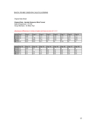
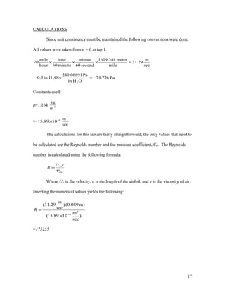
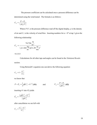
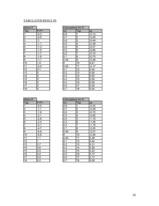
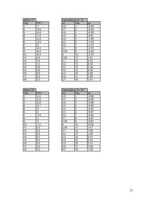
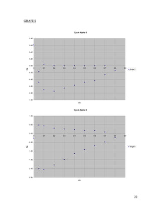
Jean-Paul Gibson: Aerolab Subsonic Wind Tunnel Report

THERMO/FLUIDS LAB ME 415
AEROLAB SUBSONIC
WIND TUNNEL
ME 415 Lab
Instructor: Dr. Ross
Group Members: Mikel, Albern, Paul
Date of Experiment: 2/11/02
Date of Report: 3/4/02
Mikel: pp 12, 24-25, 25a-25d,

Albern: pp 11, 14, 26, 28-29, 30
Paul: pp 1-3, 5-9, 16-22
2

TABLE OF CONTENTS
Abstract 3
Theory 5
Published Results 9
Equipment 11
Procedure 12
Data for Calculations 14
Analysis 16
Tabulated Results with Graphs 19
Discussion 24
References 26
Schematic 28
Original Data Sheet 30
3

ABSTRACT
In this lab, an airfoil was tested within a subsonic wind tunnel generating winds at
70 miles per hour. Data was collected at 18 separate tap points along the airfoil in order
to calculate the pressure coefficient at each of those points. The process of gathering data
for 18 taps was repeated four times at 0°, 6°, 12° and 18° for an angle of attack. In
summary, angles 0° and 6° provided results that were reasonably close to expected
results. However, angle 12° and 18° yielded bad data that was not expected, possibly due
to inaccurate readings of pressure differential. Calculations for Cp at each of these taps
are provided in the Analysis section of this report
4

THEORY
Airfoils are sensitive and important devices. They can determine whether an
airplane will be airworthy and whether or not it will plummet into the ground. Airfoils
normally take a raindrop like shape and are symmetrical about a straight line running
through the center called the chord line. The angle at which the chord line is directed
against wind flow is referred to as the angle of attack, α. Figure 1 from reference 4
shows a diagram of a typical airfoil as well as the location of the chord line.
Figure 1
The difference between the chord line and the mean camber line is that the mean
camber line represents a curved line drawn from the leading edge back to the trailing
edge maintains equidistance between upper and bottom surfaces. Two stagnation lines
occur along an airfoil, one along the leading edge and one along the trailing edge. The
leading edge is the surface located centrally along the front edge the airfoil. It is the line
that separates whether air travels along the upper or lower surface of the airfoil. Both
these stagnation lines occur along the entire span (length into this paper) of the airfoil.
Figure 2 provides a visual representation of the locations of these stagnation points.
6

Figure 2
Truly accurate data for airfoils is very difficult to obtain in a lab environment
because of the behavior of airfoils given certain conditions. First, inaccurate and
consistent data is difficult to obtain when the Reynolds number is less than 500000.
Airfoils being tested within these conditions are much more vulnerable to outside
disturbances such as turbulence and high noise levels. With our calculated Reynolds
number of approximately 175000 being much less than 500000, we can only gather that
our data, though not incorrect, may not be entirely repeatable if the experiment was
performed again.
Secondly, although the lab called for a steady 70 mph wind speed, maintaining
this speed at exactly 70 mph is nearly impossible. The wind speed constantly fluctuated
between values that were usually slightly lower than the desired 70 mph. Furthermore,
very small changes in pressure are measured along the airfoil surface. Because of small
changes in pressure, inaccuracies in reading data can account for some large errors
occasionally.
Airfoils are capable of producing two different forces, lift and drag. If the angle
of attack is zero than either lift or drag is produced. Lift occurs when flow along the
upper surface is greater than the flow along the lower surface. Conversely, drag occurs
when flow is greater on the lower surface than on the upper surface. Forces are
7

dependent on both the pressure distribution surrounding the airfoil as well as the Mach
number. However, since this experiment was performed well below the supersonic
threshold, the Mach number was not a governing factor. Figure 3 from reference 4
depicts foils producing both drag and lift. The top wing is producing drag while the
middle and bottom ones are producing lift. The number to right denotes the angle of
attack. Typically, the lift or drag force that an airfoil is capable of producing is given as a
nondimensional number rather than a vector quantity. Both the lift and drag coefficients
be calculated using the following formulae:
SV
D
C
SV
L
C DL 2
2
12
2
1
∞∞ ρ
=
ρ
=
Where L is the lift force, D is the drag force, ρ is the density of air, V∞ is the air velocity
and S is the surface roughness.
Figure 3
8

Knowing both the coefficient of drag and the coefficient lift one can determine
the lift-drag ratio:
2
2






+α
α
=
c
tC
C
D
L
Where t represents the thickness of the airfoil. This equation is only valid for two
conditions:
I. The airfoil must be thin, meaning its thickness is much less than its chord line.
II. The angle of attack must be kept reasonably small.
One can also calculate the maximum lift-drag coefficient using the following
formula. The largest possible ratio occurs when α = t/c.






=





c
tC
C
D
L
2
1
max
9

PUBLISHED RESULTS
Published results can be located in the lab manual provided for this experiment.
10

EQUIPMENT
1. Aerolab Wind tunnel
2. Airfoil
3. Digital readout differential pressure sensor.
12

PROCEDURE
1. Set the lab equipment as described in the EQUIPMENT section.
2. Measure and record the dimensions of the airfoil, and the position of each tap.
3. Set the airfoil at the correct angle, making sure it is ascending, not diving (0, 6, 12
and 18 degrees for the three runs)
4. If the wind tunnel controls were not set up, follow the instructions below:
5. Turn ON the control panel box. Activate Polyspede control: Turn ON the power
vial rod to ceiling box. Set controls using the following sequence:
Mon
F SET M Terminal, STR
F/R SW Ope-Key STR
FM 000 Hz, STR
FS 000 Hz, STR
Also press FWD/RUN, STR
6. Check the airfoil to make sure it’s properly secured
7. Close and secure the observation door.
8. Increase the air speed (U) to 70MPH. Speed should remain constant throughout
the experiment.
9. Using the selector (located to the left of the control panel), select each pressure
tap and record the pressure reading for all the taps on the airfoil.
10. Repeat the experiment for all four angles of attack.
13

DATA TO BE USED IN CALCULATIONS
14

DATA TO BE USED IN CALCULATIONS
Original Data Sheet
Original Data: Aerolab Subsonic Wind Tunnel
Data of Experiment: 2/11/02
Group Members: Al, Mikel, Paul
all pressure differences in inches of water and have an error of +/- 0.1
Alpha Tap 1 Tap 2 Tap 3 Tap 4 Tap 5 Tap 6 Tap 7 Tap 8 Tap 9
0 -0.3 -0.6 -1 -1.1 -1.3 -1.5 -1.7 -1.6 -1.1
6 -0.5 -1.1 -1.6 -2.1 -2.6 -3.4 -4.1 -4.7 -4.6
12 -1 -0.9 -0.9 -1.4 -2.4 -3.5 -5 -6.3 -6.4
18 -2.2 -2.2 -2.2 -2.1 -2 -2 -1.9 -2 -2
Alpha Tap 10 Tap 11 Tap 12 Tap 13 Tap 14 Tap 15 Tap 16 Tap 17 Tap 18
0 1.4 -0.4 0.1 0 0 0 0 0 0
6 -0.6 1.1 1 0.7 0.6 0.5 0.4 0.4 0.2
12 -6.3 2.3 1.6 1.2 0.9 0.8 0.6 2.4 2.3
18 -1.2 2.3 2.4 2.4 0.7 0.5 0.3 2.4 2.5
15

CALCULATIONS
Since unit consistency must be maintained the following conversions were done.
All values were taken from α = 0 at tap 1.
sec
m
31.29
mile
meter1609.344
second60
minute
minute60
hour
hour
mile
70 =×××
Pa74.726
OHin
Pa249.08891
OHin0.3
2
2 −=×−
Constants used:
ρ=1.164 3
m
kg
ν=
sec
m
1015.89
2
6−
×
The calculations for this lab are fairly straightforward; the only values that need to
be calculated are the Reynolds number and the pressure coefficient, Cp. The Reynolds
number is calculated using the following formula:
air
cU
R
ν
∞
=
Where U∞ is the velocity, c is the length of the airfoil, and ν is the viscosity of air.
Inserting the numerical values yields the following:
)
sec
m
1089.15(
)m089.0()
sec
m
29.31(
2
6−
×
=R
=175255
17

The pressure coefficient can be calculated once a pressure difference can be
determined using the wind tunnel. The formula is as follows:
2
2
1
∞
∞−
=
U
PP
C
air
p
ρ
Where P-P∞ is the pressure difference read off the digital display, ρ is the density
of air and U∞ is the velocity of wind flow. Inserting numbers for α = 0° at tap 1 gives the
following relationship:
2
32
1
2
)
sec
m
29.31)(
m
kg
164.1(
m
N
726.74
=pC
=0.1311
Calculations for all other taps and angles can be found in the Tabulated Results
section.
Using Bernoulli’s equation one can derive the following equation:
2
2
1
∞
−=
U
U
Cp
we know that
( )22
2
1
UUPP −ρ=− ∞∞ (#1) and 2
2
1
∞
∞
ρ
−
=
U
PP
Cp (#2)
inserting #1 into #2 yields
( )
2
2
1
22
2
1
∞
∞
ρ
−ρ
=
U
UU
Cp
after cancellation we are left with
2
22
∞
∞ −
=
U
UU
Cp
18

expanding the result by using a common denominator gives us our desired equation of
2
2
1
∞
−=
U
U
Cp
Deriving the other equation is done in a similar fashion using substitution. First,
we start with the equation below:
( )22
2
1
UUPP −ρ=− ∞∞
bring the P∞ to the right side of the equation as shown below
( )22
2
1
UUPP −ρ+= ∞∞
divide by ρ
( )
ρ
−ρ
+
ρ
=
ρ
∞
∞
22
2
1
UU
PP
canceling out the ρ leaves
( )22
2
1
UU
PP
−+
ρ
=
ρ
∞
∞
expand the parenthesis
22
22
UUPP
++
ρ
=
ρ
∞∞
the U2
cancels out and we are left with the desired relationship
2
2
∞∞
+
ρ
=
ρ
UPP
19

TABULATED RESULTS
Alpha 0° Calculations for 0°
Tap P-P∞ x/c Tap cp
1 -0.3 0.8 1 -0.13
2 -0.6 0.7 2 -0.26
3 -1 0.6 3 -0.44
4 -1.1 0.5 4 -0.48
5 -1.3 0.4 5 -0.57
6 -1.5 0.3 6 -0.66
7 -1.7 0.2 7 -0.74
8 -1.6 0.1 8 -0.70
9 -1.1 0.05 9 -0.48
10 1.4 0 10 0.61
11 -0.4 0.05 11 -0.17
12 0.1 0.1 12 0.04
13 0 0.2 13 0.00
14 0 0.3 14 0.00
15 0 0.4 15 0.00
16 0 0.5 16 0.00
17 0 0.6 17 0.00
18 0 0.7 18 0.00
1 -0.5 0.8 1 -0.22
2 -1.1 0.7 2 -0.48
3 -1.6 0.6 3 -0.70
4 -2.1 0.5 4 -0.92
5 -2.6 0.4 5 -1.14
6 -3.4 0.3 6 -1.49
7 -4.1 0.2 7 -1.79
8 -4.7 0.1 8 -2.05
9 -4.6 0.05 9 -2.01
10 -0.6 0 10 -0.26
11 1.1 0.05 11 0.48
12 1 0.1 12 0.44
13 0.7 0.2 13 0.31
14 0.6 0.3 14 0.26
15 0.5 0.4 15 0.22
16 0.4 0.5 16 0.17
17 0.4 0.6 17 0.17
18 0.2 0.7 18 0.09
20

1 -1 0.8 1 -0.44
2 -0.9 0.7 2 -0.39
3 -0.9 0.6 3 -0.39
4 -1.4 0.5 4 -0.61
5 -2.4 0.4 5 -1.05
6 -3.5 0.3 6 -1.53
7 -5 0.2 7 -2.19
8 -6.3 0.1 8 -2.75
9 -6.4 0.05 9 -2.80
10 -6.3 0 10 -2.75
11 2.3 0.05 11 1.01
12 1.6 0.1 12 0.70
13 1.2 0.2 13 0.52
14 0.9 0.3 14 0.39
15 0.8 0.4 15 0.35
16 0.6 0.5 16 0.26
17 2.4 0.6 17 1.05
18 2.3 0.7 18 1.01
1 -2.2 0.8 1 -0.96
2 -2.2 0.7 2 -0.96
3 -2.2 0.6 3 -0.96
4 -2.1 0.5 4 -0.92
5 -2 0.4 5 -0.87
6 -2 0.3 6 -0.87
7 -1.9 0.2 7 -0.83
8 -2 0.1 8 -0.87
9 -2 0.05 9 -0.87
10 -1.2 0 10 -0.52
11 2.3 0.05 11 1.01
12 2.4 0.1 12 1.05
13 2.4 0.2 13 1.05
14 0.7 0.3 14 0.31
15 0.5 0.4 15 0.22
16 0.3 0.5 16 0.13
17 2.4 0.6 17 1.05
18 2.5 0.7 18 1.09
21

GRAPHS
Cp at Alpha 0
-1.00
-0.80
-0.60
-0.40
-0.20
0.00
0.20
0.40
0.60
0.80
0 0.1 0.2 0.3 0.4 0.5 0.6 0.7 0.8 0.9
x/c
Cp
Angle 0
Cp at Alpha 6
-2.50
-2.00
-1.50
-1.00
-0.50
0.00
0.50
1.00
0 0.1 0.2 0.3 0.4 0.5 0.6 0.7 0.8 0.9
x/c
Cp
Angle 6
22

Cp at Alpha 12
-3.00
-2.50
-2.00
-1.50
-1.00
-0.50
0.00
0.50
1.00
1.50
0 0.1 0.2 0.3 0.4 0.5 0.6 0.7 0.8 0.9
x/c
Cp
Angle 12
Cp at Alpha 18
-1.50
-1.00
-0.50
0.00
0.50
1.00
1.50
0 0.1 0.2 0.3 0.4 0.5 0.6 0.7 0.8 0.9
x/c
Cp
Angle 18
23

DISCUSSION
1.- a) Why is the maximum value of Cp one?
Given that 2
2
1
∞
−=
U
U
Cp We can see that if the local air speed (U)
becomes very large compared to the absolute air speed, Cp becomes negative. If U is less
than U∞, Cp will be one (if U is zero) or less than one.
b) Why is Cp = 1 at the stagnation point?
If U becomes zero (at the stagnation point), by using
2
2
1
∞
−=
U
U
Cp Cp becomes 1.
c) How large does U have to be for Cp to be positive or negative?
As explained in point A, if U>>U∞, Cp will be negative. If U<U∞, Cp will be
positive, but less than one.
2.- Our results compared to figure 4-15
Our diagram for angles 0° and 6° degrees seem to follow Burtin and Smith’s data.
For the 12° and 18° degree runs, our data seems to coincide with figure 4-
15, but in the 0.5-1 range for x/c, we get some deviation that does not follow
figure 4-15.
3.- Why is the pressure changing at different angles of attack?
By changing the angle of attack, we force the air traveling on the airfoil to take a
longer path. This increases the speed of the air, and using Bernoulli’s equation,
we can see that pressure decreases.
2
2
∞∞
+=
UPPatm
ρρ
The greater the angle of attack, the greater the air speed on the upper side of the
airfoil, and the lower the local pressure will be.
25

4.- Where is the boundary separation point of the plot for an angle of attack of 12
degrees?
If as described, this point is located at the area where pressure remains constant,
this will be between 0.3<x/c<0.5.
5.- Refer to page 25d
26

REFERENCES
1. Fundamentals of Heat and Mass Transfer. Frank P. Incropera, David P. DeWitt.
John Wiley & Sons, New York, 1996
2. ME 415 Lab notes. Prof. Ross.
3. ME 404 class notes.
4. http://www.monmouth.com/~jsd/how/htm/airfoils.html.
5. Compressible Fluid Flow. Sadd, Michel A. Prentice Hall. Upper Saddle River,
NJ, 07458. 1993.
6. Fluid Mechanics. Ahmed, Nazeer. Engineering Press Inc., San Jose, CA. 1987.
27

SCHEMATICS
Figure 4
Figure 5
29

Figure 6
Figure 7
Figure 4: Aerolab airfoil chamber.
Figure 5: Aerolab tap number selector knob.
Figure 6: Digital readout for pressure differential.
Figure 7: Close up of connection for digital readout to Aerolab wind tunnel.
30

Jean-Paul Gibson: Aerolab Subsonic Wind Tunnel Report

More Related Content

What's hot

Viewers also liked

Similar to Jean-Paul Gibson: Aerolab Subsonic Wind Tunnel Report

Recently uploaded

Jean-Paul Gibson: Aerolab Subsonic Wind Tunnel Report