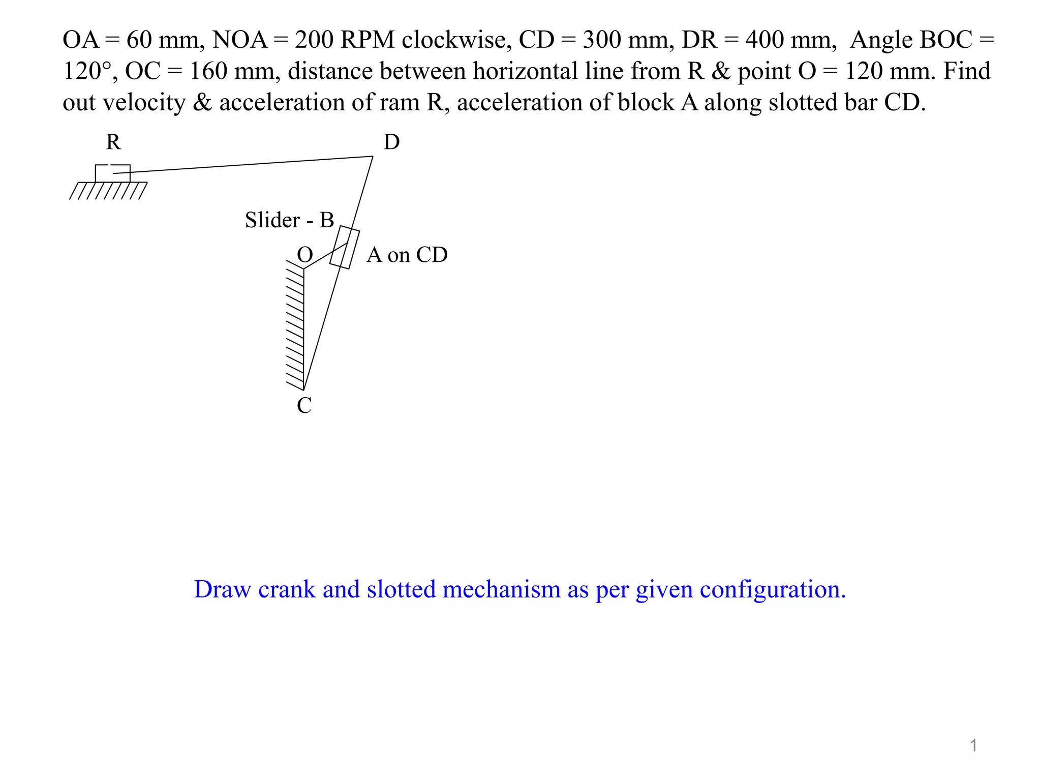
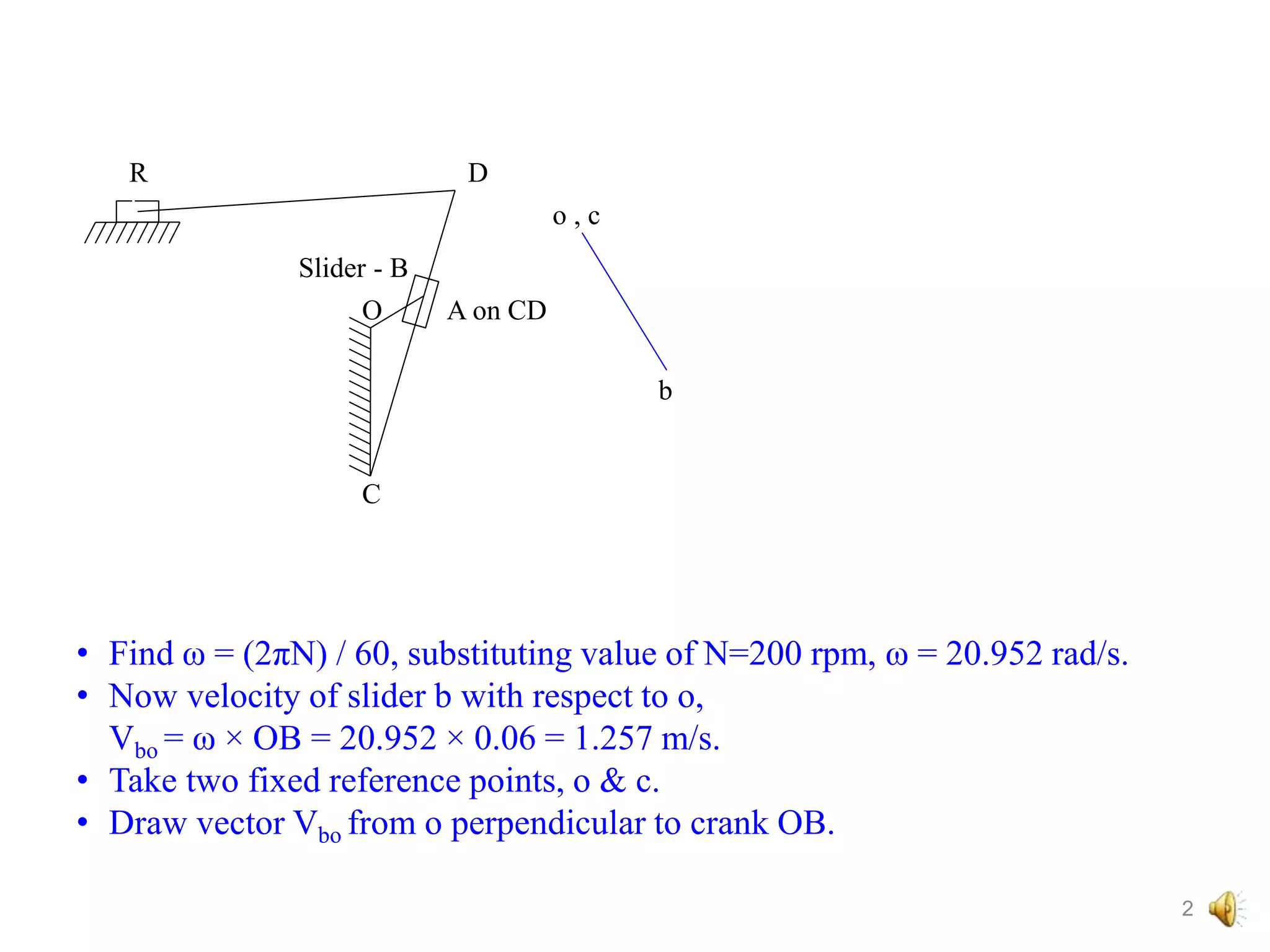
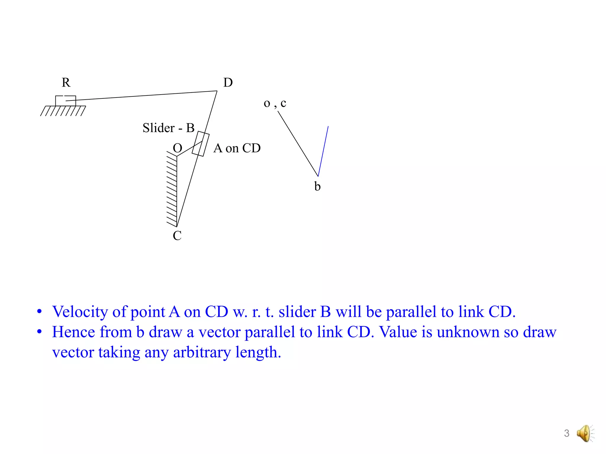
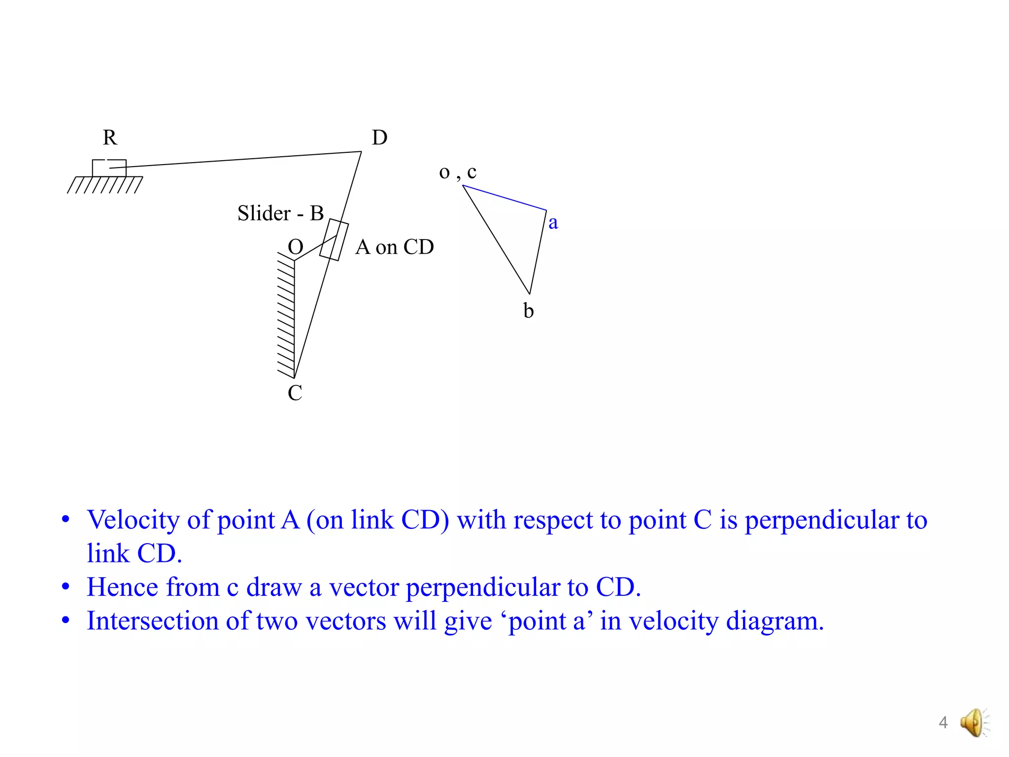
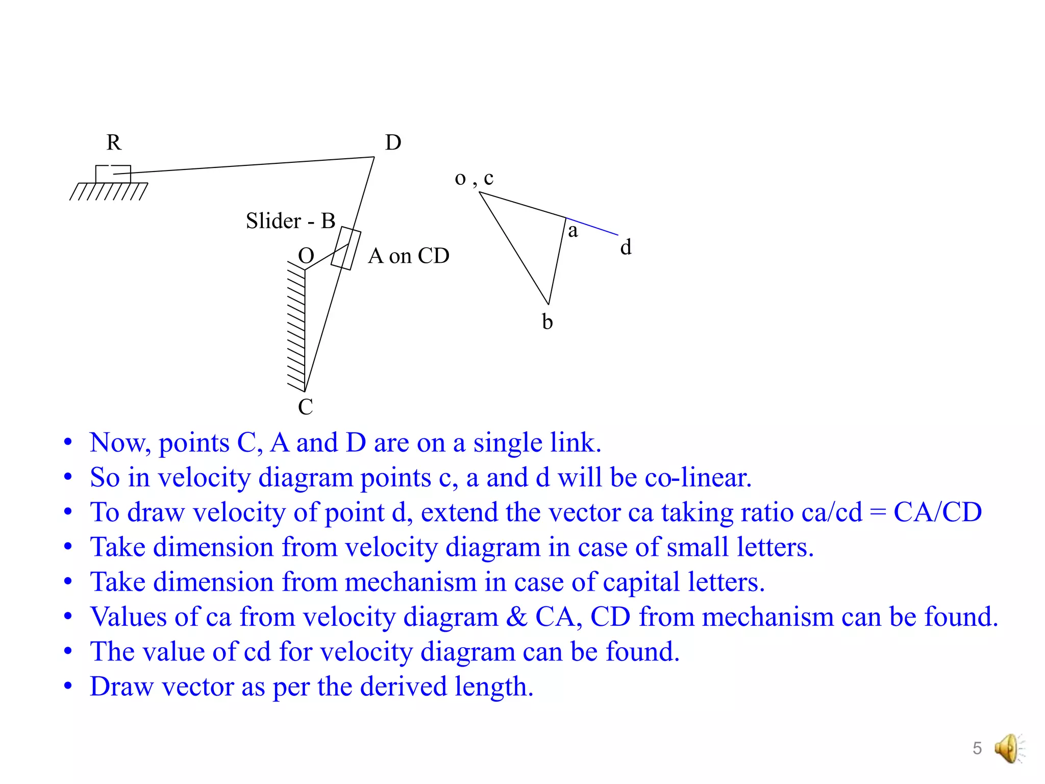
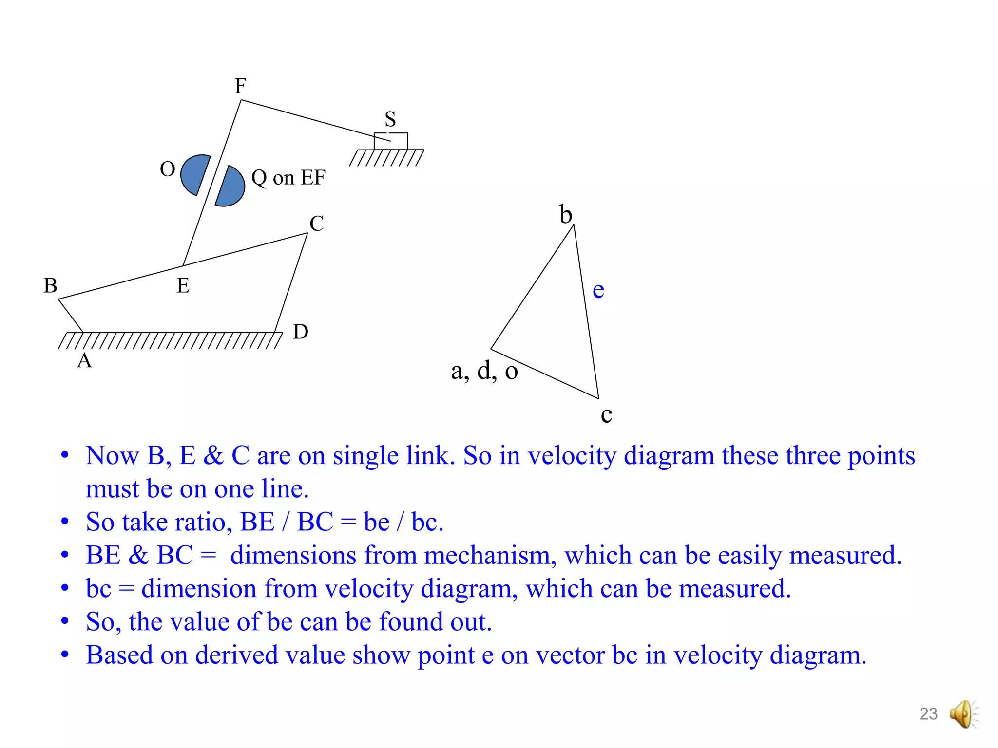
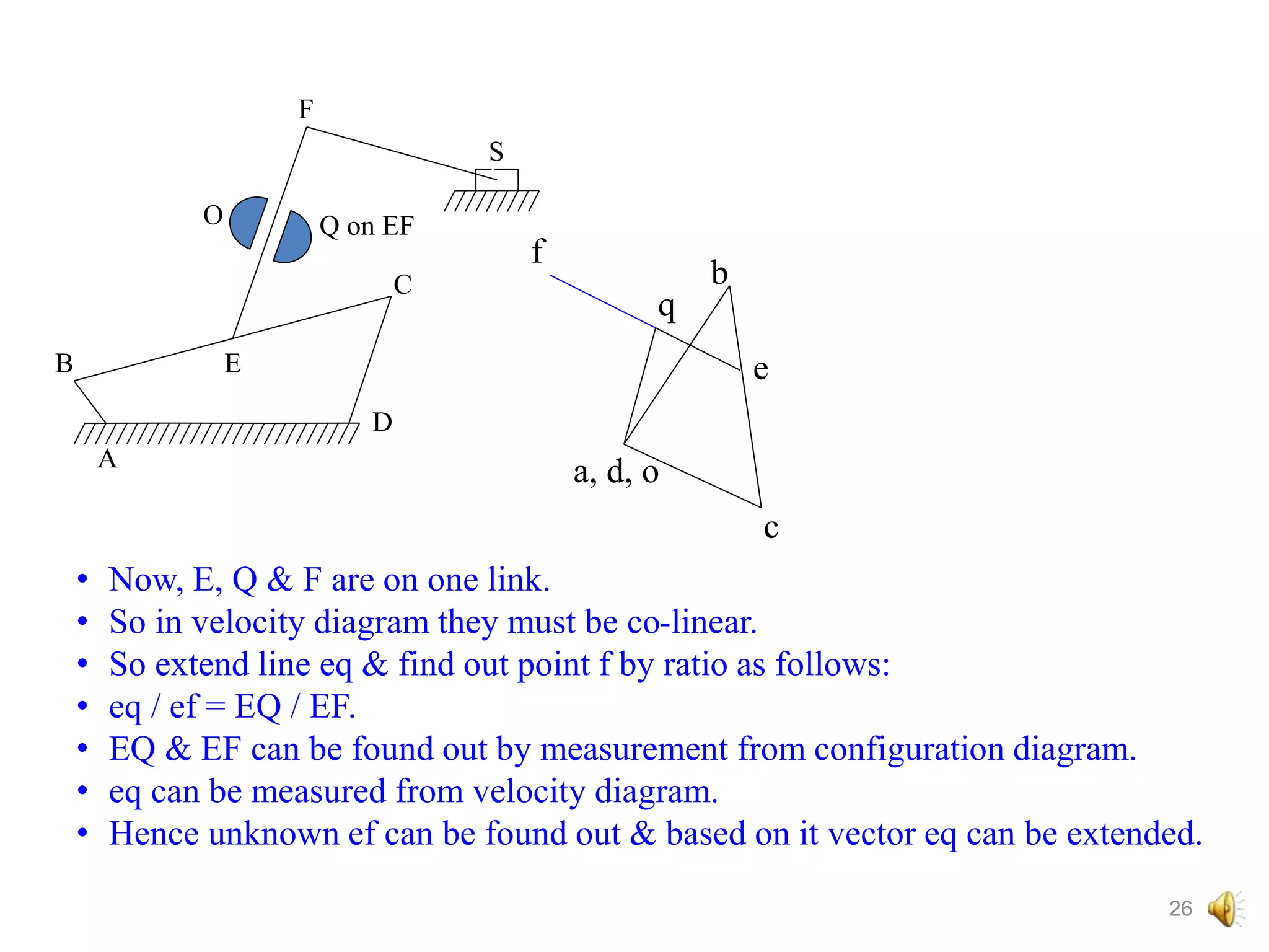
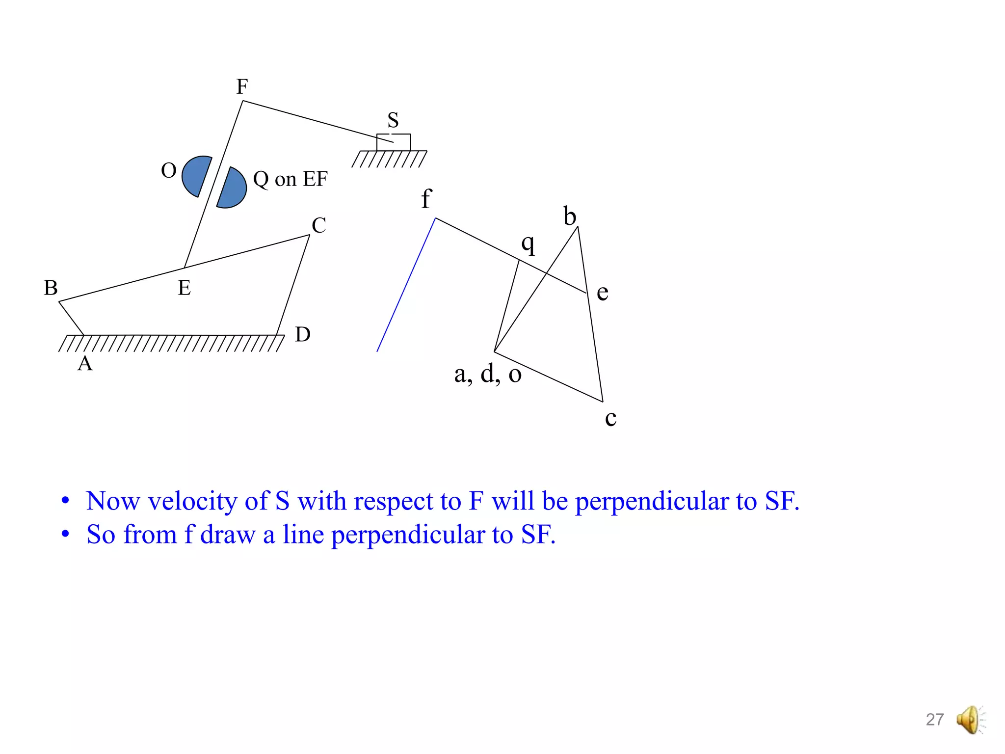
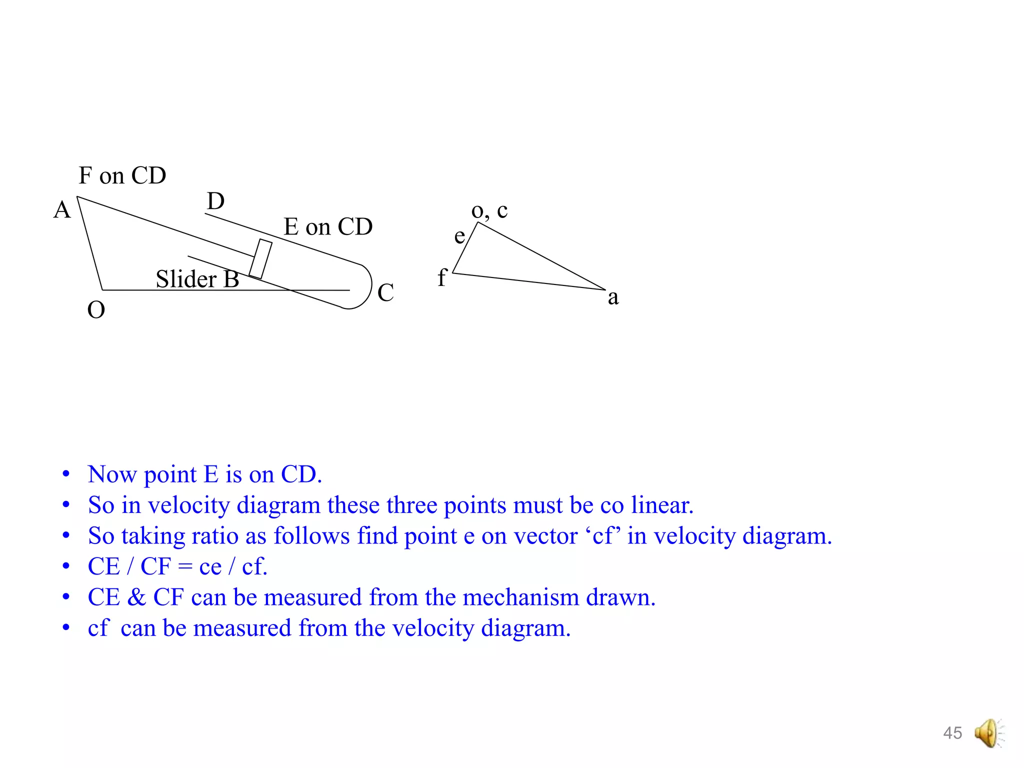
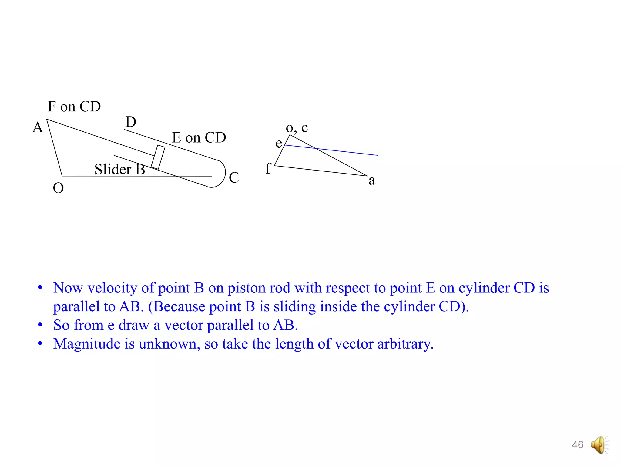
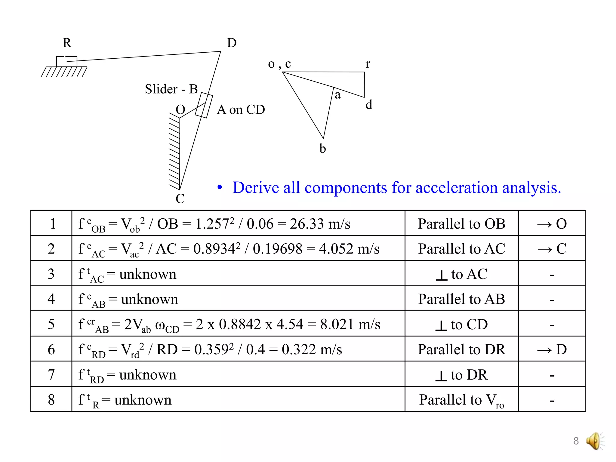
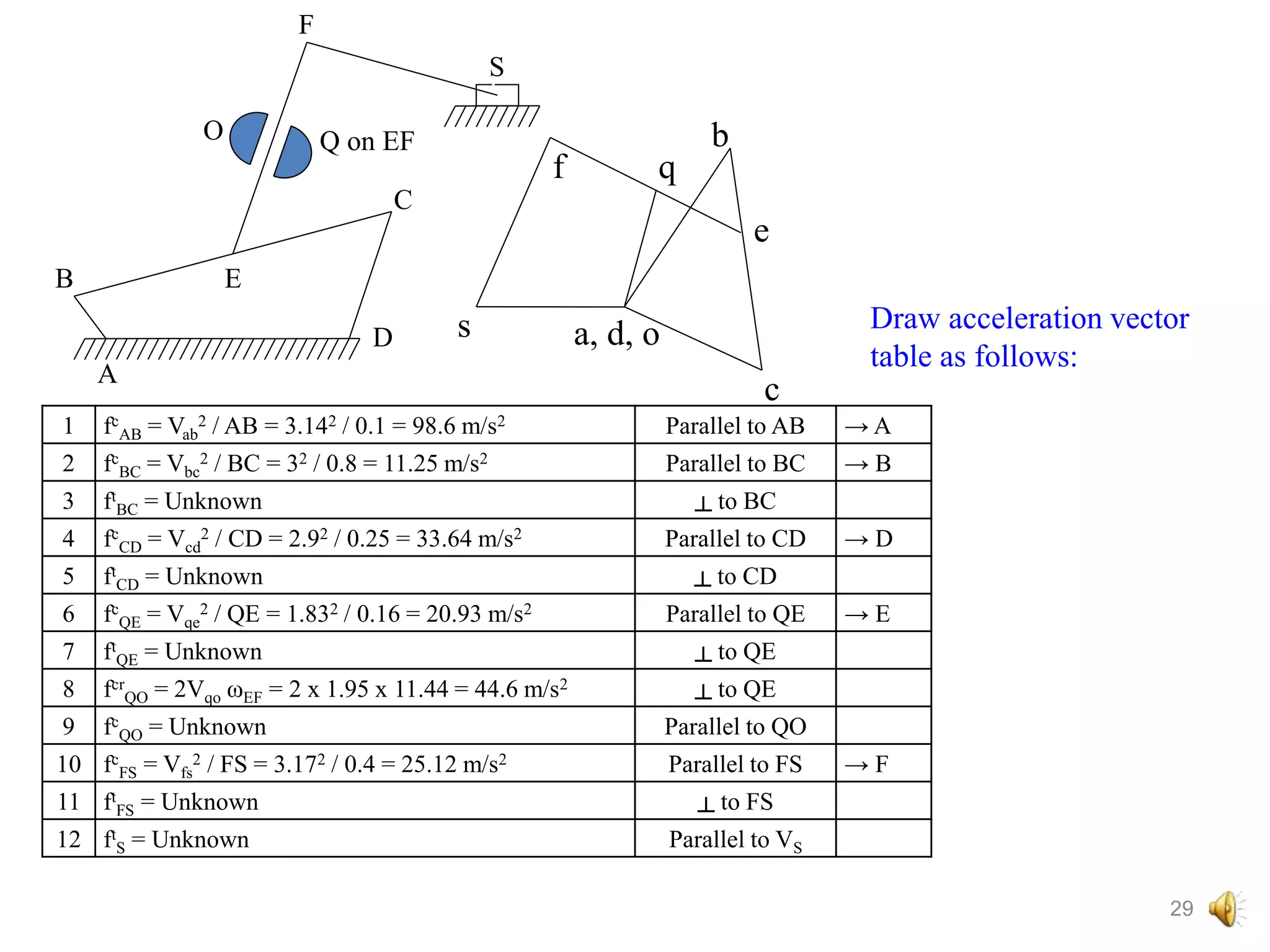
This document provides instructions for drawing velocity and acceleration diagrams for a slider-crank mechanism. It includes the following key steps: 1. Calculate angular velocity and linear velocities of points using given dimensions and rotational speed. 2. Draw velocity vectors in the velocity diagram showing velocities of all points relative to fixed references and each other. 3. Derive accelerations of points from the velocity diagram and mechanism dimensions. 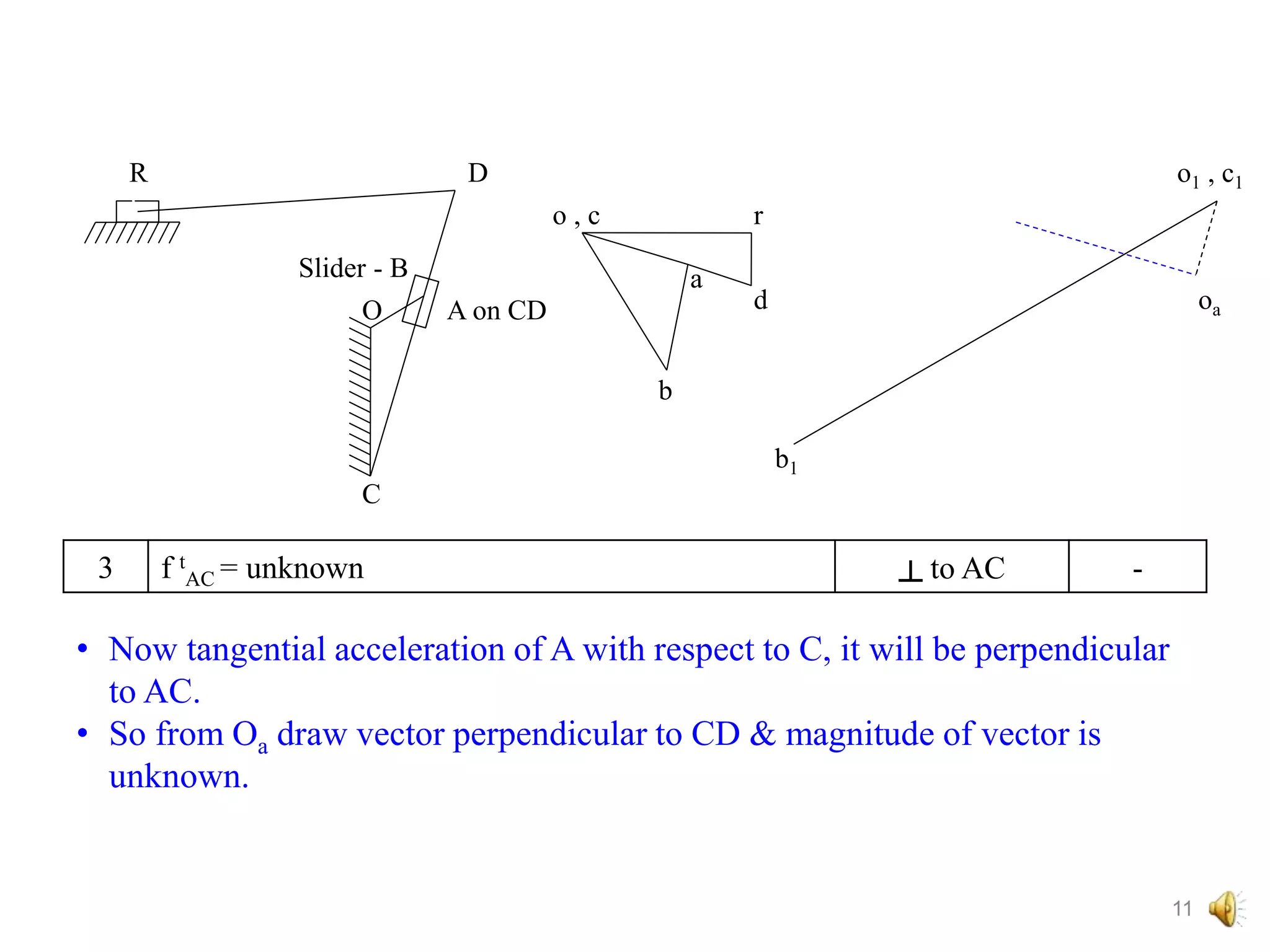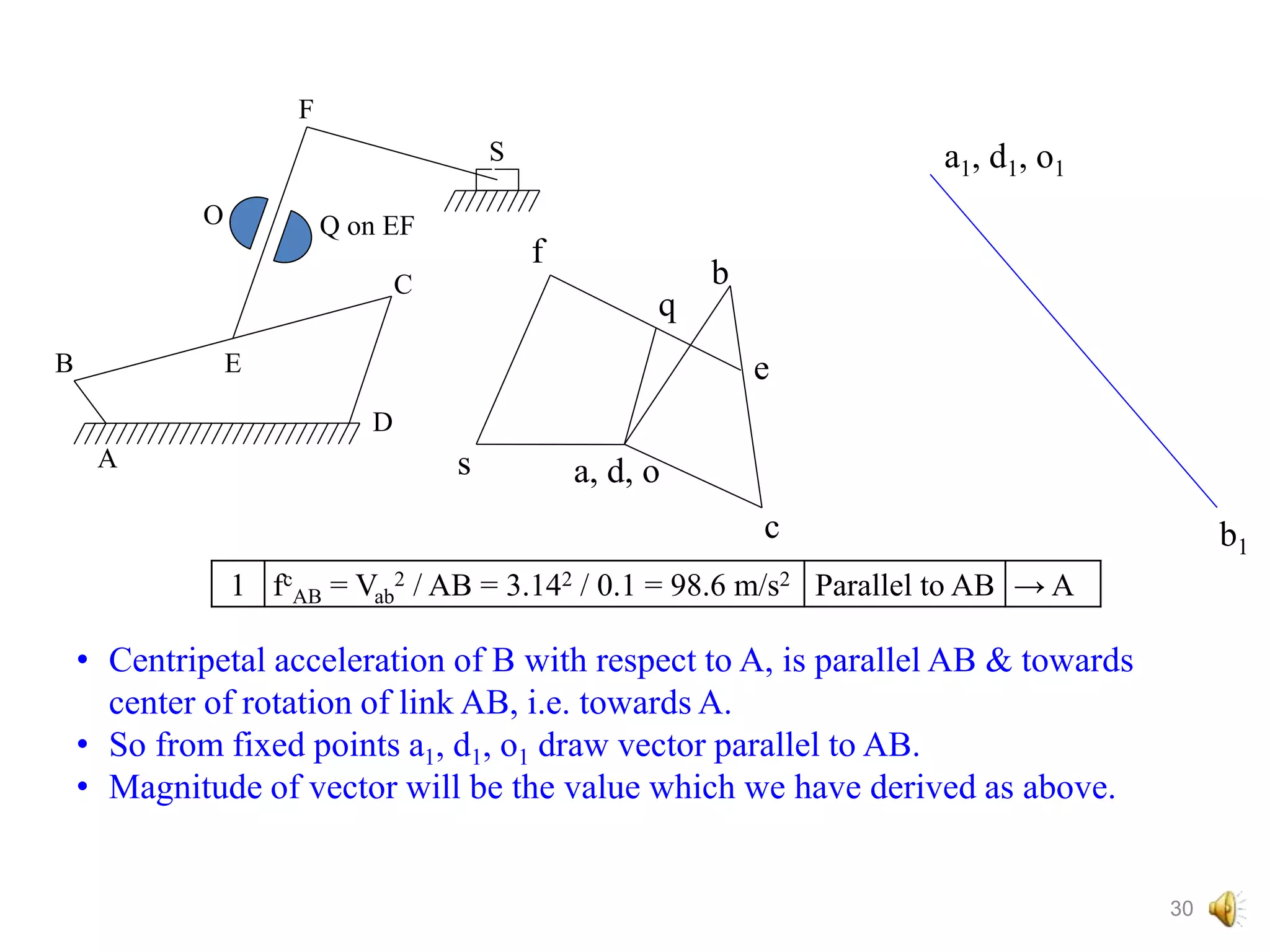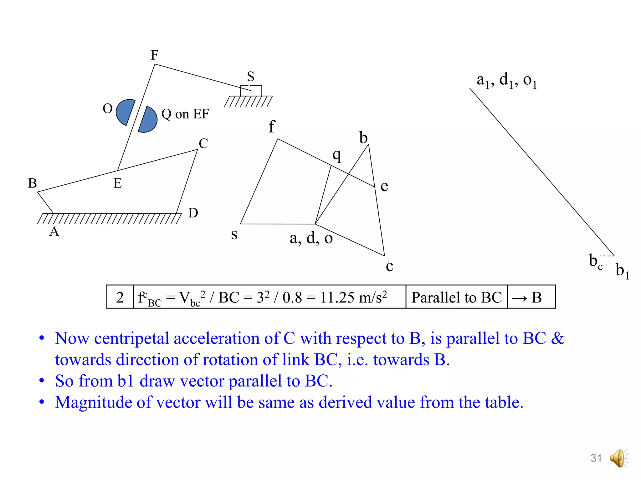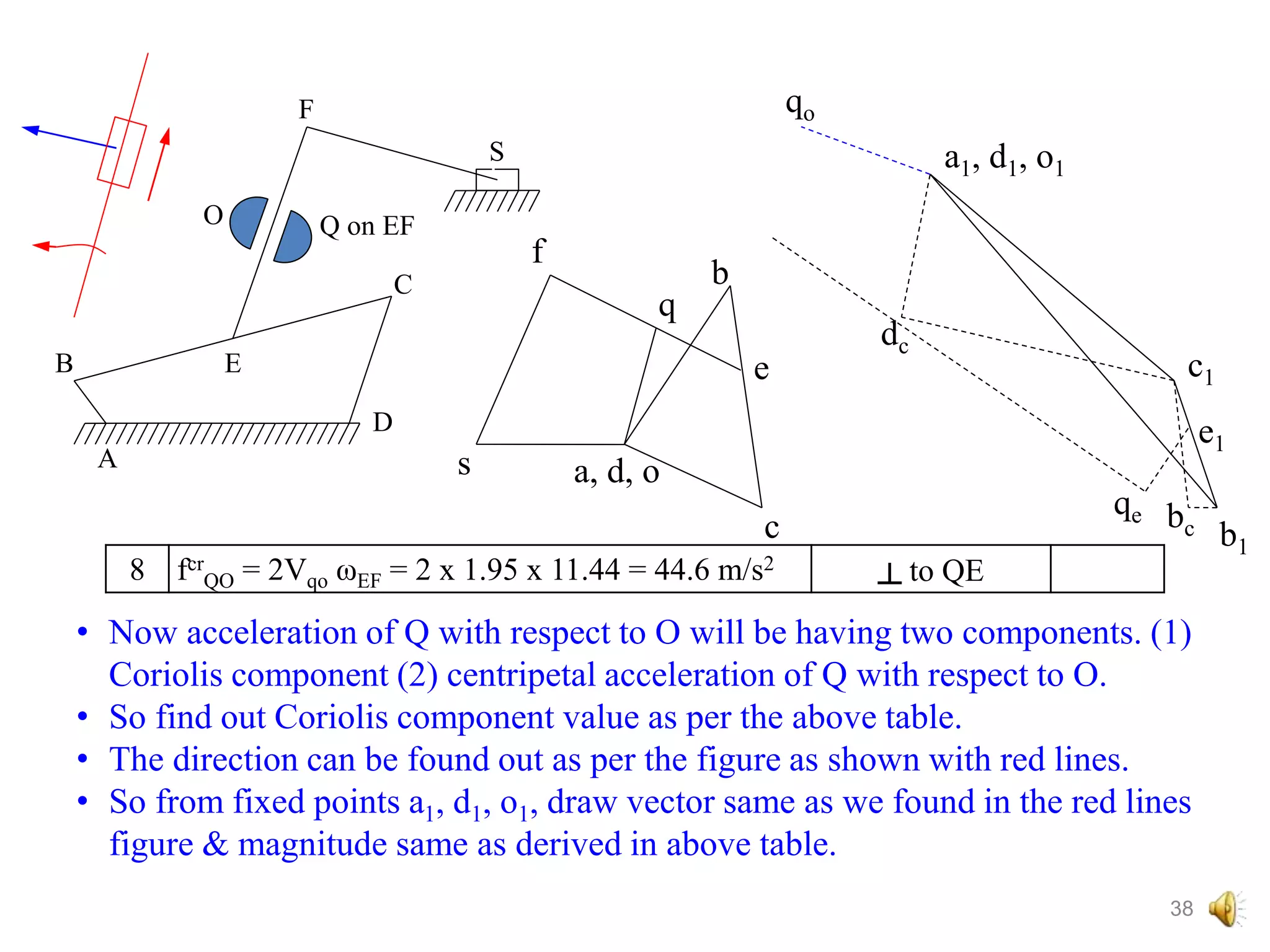4. Draw acceleration vectors in the acceleration diagram showing centripetal, tangential, and coriolis accelerations of all points.

1. P
r
O
C
Slider - B
A on CD
DR
Draw crank and slotted mechanism as per given configuration.
OA = 60 mm, NOA = 200 RPM clockwise, CD = 300 mm, DR = 400 mm, Angle BOC =
120°, OC = 160 mm, distance between horizontal line from R & point O = 120 mm. Find
out velocity & acceleration of ram R, acceleration of block A along slotted bar CD.
1

2. P
r
O
C
Slider - B
A on CD
DR
o , c
b
• Find ω = (2πN) / 60, substituting value of N=200 rpm, ω = 20.952 rad/s.
• Now velocity of slider b with respect to o,
Vbo = ω × OB = 20.952 × 0.06 = 1.257 m/s.
• Take two fixed reference points, o & c.
• Draw vector Vbo from o perpendicular to crank OB.
2

3. P
r
O
C
Slider - B
A on CD
DR
o , c
b
• Velocity of point A on CD w. r. t. slider B will be parallel to link CD.
• Hence from b draw a vector parallel to link CD. Value is unknown so draw
vector taking any arbitrary length.
3

4. P
r
O
C
Slider - B
A on CD
DR
o , c
b
a
• Velocity of point A (on link CD) with respect to point C is perpendicular to
link CD.
• Hence from c draw a vector perpendicular to CD.
• Intersection of two vectors will give ‘point a’ in velocity diagram.
4

5. P
r
O
C
Slider - B
A on CD
DR
o , c
b
a
• Now, points C, A and D are on a single link.
• So in velocity diagram points c, a and d will be co-linear.
• To draw velocity of point d, extend the vector ca taking ratio ca/cd = CA/CD
• Take dimension from velocity diagram in case of small letters.
• Take dimension from mechanism in case of capital letters.
• Values of ca from velocity diagram & CA, CD from mechanism can be found.
• The value of cd for velocity diagram can be found.
• Draw vector as per the derived length.
d
5

6. P
r
O
C
Slider - B
A on CD
DR
o , c
b
a
d
• From d draw velocity of r with respect to point d (Vrd), perpendicular to RD.
6

7. P
r
O
C
Slider - B
A on CD
DR
o , c
b
a
d
r
• Now, velocity of slider r with respect to fixed point o or c will be in horizontal
line. So, from o or c draw horizontal line.
• Intersection of two vectors will be point r.
7

8. P
r
O
C
Slider - B
A on CD
DR
o , c
b
a
d
r
1 f c
OB = Vob
2 / OB = 1.2572 / 0.06 = 26.33 m/s Parallel to OB → O
2 f c
AC = Vac
2 / AC = 0.89342 / 0.19698 = 4.052 m/s Parallel to AC → C
3 f t
AC = unknown ┴ to AC -
4 f c
AB = unknown Parallel to AB -
5 f cr
AB = 2Vab ωCD = 2 x 0.8842 x 4.54 = 8.021 m/s ┴ to CD -
6 f c
RD = Vrd
2 / RD = 0.3592 / 0.4 = 0.322 m/s Parallel to DR → D
7 f t
RD = unknown ┴ to DR -
8 f t
R = unknown Parallel to Vro -
• Derive all components for acceleration analysis.
8

9. P
r
O
C
Slider - B
A on CD
DR
o , c
b
a
d
r
o1 , c1
b1
• From acceleration table draw 1st acceleration vector.
• Centripetal acceleration of slider B with respect of O, will be parallel to OB &
it will be toward centre of rotation of link OB, i.e. O.
• So from O1 draw vector parallel to OB & head of vector towards O.
• Magnitude of vector will be same as the value which we have found.
1 f c
OB = Vob
2 / OB = 1.2572 / 0.06 = 26.33 m/s Parallel to OB → O
9

10. P
r
O
C
Slider - B
A on CD
DR
o , c
b
a
d
r
o1 , c1
b1
oa
22 f c
AC = Vac
2 / AC = 0.89342 / 0.19698 = 4.052 m/s Parallel to AC → C
• Now centripetal acceleration of A with respect to C, it will be parallel to AC
& towards the centre of rotation of link AC, i.e. towards C.
• So from C1 draw vector parallel to CD & magnitude of vector will be as per
the value derived.
10

11. P
r
O
C
Slider - B
A on CD
DR
o , c
b
a
d
r
o1 , c1
b1
oa
3 f t
AC = unknown ┴ to AC -
• Now tangential acceleration of A with respect to C, it will be perpendicular
to AC.
• So from Oa draw vector perpendicular to CD & magnitude of vector is
unknown.
11

12. P
r
O
C
Slider - B
A on CD
DR
o , c
b
a
d
r
o1 , c1
b1
ba
oa
5 f cr
AB = 2Vab ωCD = 2 x 0.8842 x 4.54 = 8.021 m/s ┴ to CD -
• Here we are interested in finding out acceleration of slider B with respect to
C. It is addition of acceleration of B with respect to A & acceleration of A
with respect to C.
• Here coriolis component will come into picture.
• It can be found our by the method shown in red figure. Blue vector is coriolis
component of acceleration.
• Pick coriolis component & put its head at b1. 12

13. P
r
O
C
Slider - B
A on CD
DR
o , c
b
a
d
r
o1 , c1
b1
ba
oa
a1
4 f c
AB = unknown Parallel to AB -
• From ba draw centripetal acceleration of B with respect to A.
• Draw a line parallel to CD from ba.
• Intersection of two vectors will be point a1.
13

14. P
r
O
C
Slider - B
A on CD
DR
o , c
b
a
d
r
o1 , c1
b1
ba
oa
a1
d1
• a1b1 = Total acceleration of B with respect to A.
• c1a1 = Total acceleration of A with respect to C.
• Now links C, A & D are co-linear.
• Hence in acceleration diagram these three points must be co-linear.
• So taking ratio, c1a1/c1d1 = CA / CD.
• Capital letter indicates measurements from mechanism drawn.
• Small letter indicates measurements from acceleration diagram. 14

15. P
r
O
C
Slider - B
A on CD
DR
o , c
b
a
d
r
o1 , c1
b1
ba
oa
a1
d1
15

16. P
r
O
C
Slider - B
A on CD
DR
o , c
b
a
d
r
o1 , c1
b1
ba
oa
a1
d1 rd
6 f c
RD = Vrd
2 / RD = 0.3592 / 0.4 = 0.322 m/s Parallel to DR → D
• Now draw centripetal component of point R with respect to D. It is parallel to
DR & it is towards centre of rotation of link DR, i.e. towards D.
• Do from rd draw a line parallel to DR.
• Magnitude is same as the derived one.
d1 rd
16

17. P
r
O
C
Slider - B
A on CD
DR
o , c
b
a
d
r
o1 , c1
b1
ba
oa
a1
d1 rd
7 f t
RD = unknown ┴ to DR -
• Now tangential acceleration of point R with respect to D.
• Value is unknown.
• So from rd draw a line perpendicular to DR.
17

18. P
r
O
C
Slider - B
A on CD
DR
o , c
b
a
d
r
o1 , c1
b1
ba
oa
a1
d1
r1
rd
8 f t
R = unknown Parallel to Vro -
• Now draw tangential acceleration of slider R.
• Value is unknown.
• From c1 draw a horizontal line.
• Intersection of two points will be point r1.
18

19. P
r
O
C
Slider - B
A on CD
DR
o , c
b
a
d
r
o1 , c1
b1
ba
oa
a1
d1
r1
rd
Configuration Diagram
Velocity
Diagram
Acceleration
Diagram
19

20. P
r
D
A
C
B E
Q on EFO
F
S
a, d, o
b
• Draw configuration diagram as per given dimensions.
• Speed of crank AB in rpm is given.
• So find out angular velocity of link AB, ω = (2πN) / 60.
• Now find velocity of B with respect to A, Vba = ω x AB.
• Now Vba is perpendicular to AB.
• So, from the fixed points a, d, o draw vector perpendicular to AB &
magnitude = Vba.
400
400
300
AD = 650 mm, AB = 100 mm, BC = 800 mm, DC = 250 mm, BE=CE, EF = 400 mm,
FO = 240 mm, FS = 400 mm, Angle BAD = 135°. NAB = 300 RPM Clockwise. Find
acceleration of sliding of link EF in trunion.
20

21. P
r
D
A
C
B E
Q on EFO
F
S
a, d, o
b
• Now velocity of C with respect to B will be perpendicular to BC.
• So from B draw a line perpendicular to BC.
21

22. P
r
D
A
C
B E
Q on EFO
F
S
a, d, o
c
b
• Now velocity of C with respect to D will be perpendicular to CD.
• So from d draw a line perpendicular to CD.
• Intersection of two velocity vector (1) velocity of C with respect to B & (2)
velocity if C with respect to D will be point c in velocity diagram.
22

23. P
r
D
A
C
B E
Q on EFO
F
S
a, d, o
c
e
b
• Now B, E & C are on single link. So in velocity diagram these three points
must be on one line.
• So take ratio, BE / BC = be / bc.
• BE & BC = dimensions from mechanism, which can be easily measured.
• bc = dimension from velocity diagram, which can be measured.
• So, the value of be can be found out.
• Based on derived value show point e on vector bc in velocity diagram.
23

24. P
r
D
A
C
B E
Q on EFO
F
S
a, d, o
c
e
b
• Now velocity of q with respect to E will be perpendicular to EQ.
• So from e draw vector perpendicular to EQ.
24

25. P
r
D
A
C
B E
Q on EFO
F
S
a, d, o
c
q
e
b
• Now velocity of Q with respect to O, is parallel to EQ.
• So from o draw a line parallel to EQ.
• Intersection of two vectors (1) velocity of Q with respect to E, (2) velocity of
Q with respect to O, will be point q in velocity diagram.
25

26. P
r
D
A
C
B E
Q on EFO
F
S
a, d, o
f
c
q
e
b
• Now, E, Q & F are on one link.
• So in velocity diagram they must be co-linear.
• So extend line eq & find out point f by ratio as follows:
• eq / ef = EQ / EF.
• EQ & EF can be found out by measurement from configuration diagram.
• eq can be measured from velocity diagram.
• Hence unknown ef can be found out & based on it vector eq can be extended.
26

27. P
r
D
A
C
B E
Q on EFO
F
S
a, d, o
f
c
q
e
b
• Now velocity of S with respect to F will be perpendicular to SF.
• So from f draw a line perpendicular to SF.
27

28. P
r
D
A
C
B E
Q on EFO
F
S
a, d, os
f
c
q
e
b
• Now velocity of S with respect to fixed point is parallel to velocity of S.
• So from fixed point draw line parallel to velocity of S.
• Intersection of two vectors (1) velocity of S with respect to F & (2) velocity of
S with respect to fixed point will give the point s in velocity diagram.
28

29. P
r
D
A
C
B E
Q on EFO
F
S
a, d, os
f
c
q
e
b
1 fc
AB = Vab
2 / AB = 3.142 / 0.1 = 98.6 m/s2 Parallel to AB → A
2 fc
BC = Vbc
2 / BC = 32 / 0.8 = 11.25 m/s2 Parallel to BC → B
3 ft
BC = Unknown ┴ to BC
4 fc
CD = Vcd
2 / CD = 2.92 / 0.25 = 33.64 m/s2 Parallel to CD → D
5 ft
CD = Unknown ┴ to CD
6 fc
QE = Vqe
2 / QE = 1.832 / 0.16 = 20.93 m/s2 Parallel to QE → E
7 ft
QE = Unknown ┴ to QE
8 fcr
QO = 2Vqo ωEF = 2 x 1.95 x 11.44 = 44.6 m/s2
┴ to QE
9 fc
QO = Unknown Parallel to QO
10 fc
FS = Vfs
2 / FS = 3.172 / 0.4 = 25.12 m/s2 Parallel to FS → F
11 ft
FS = Unknown ┴ to FS
12 ft
S = Unknown Parallel to VS
Draw acceleration vector
table as follows:
29

30. P
r
D
A
C
B E
Q on EFO
F
S
a, d, os
f
c
q
e
b
a1, d1, o1
b1
1 fc
AB = Vab
2 / AB = 3.142 / 0.1 = 98.6 m/s2 Parallel to AB → A
• Centripetal acceleration of B with respect to A, is parallel AB & towards
center of rotation of link AB, i.e. towards A.
• So from fixed points a1, d1, o1 draw vector parallel to AB.
• Magnitude of vector will be the value which we have derived as above.
30

31. P
r
D
A
C
B E
Q on EFO
F
S
a, d, os
f
c
q
e
b
a1, d1, o1
b1
bc
2 fc
BC = Vbc
2 / BC = 32 / 0.8 = 11.25 m/s2 Parallel to BC → B
• Now centripetal acceleration of C with respect to B, is parallel to BC &
towards direction of rotation of link BC, i.e. towards B.
• So from b1 draw vector parallel to BC.
• Magnitude of vector will be same as derived value from the table.
31

32. P
r
D
A
C
B E
Q on EFO
F
S
a, d, os
f
c
q
e
b
a1, d1, o1
b1
bc
3 ft
BC = Unknown ┴ to BC
• Now tangential acceleration of C with respect to B, is perpendicular to BC.
• So, from bc draw a vector perpendicular to BC.
• Magnitude is unknown so draw line with arbitrary length.
32

33. P
r
D
A
C
B E
Q on EFO
F
S
a, d, os
f
c
q
e
b
a1, d1, o1
b1
dc
bc
4 fc
CD = Vcd
2 / CD = 2.92 / 0.25 = 33.64 m/s2 Parallel to CD → D
• Now centripetal acceleration of C with respect to D, is parallel to CD &
towards center of rotation of link CD, i.e. towards D.
• So from fixed point a1, d1, o1 draw vector in direction parallel to CD.
• The magnitude is same as the derived in above table.
33

34. P
r
D
A
C
B E
Q on EFO
F
S
a, d, os
f
c
q
e
b
a1, d1, o1
b1
c1
dc
bc
5 ft
CD = Unknown ┴ to CD
• Now tangential acceleration of C with respect to D, is perpendicular to CD.
• So from dc draw a vector perpendicular to CD.
• Intersection of two vectors (1) tangential acceleration of C with respect to B
(2) tangential acceleration of C with respect to D, will be point c1.
34

35. P
r
D
A
C
B E
Q on EFO
F
S
a, d, os
f
c
q
e
b
a1, d1, o1
b1
c1
e1
dc
bc
• Join c1a1 & c1b1.
• c1a1 = acceleration of C with respect to A.
• c1b1 = acceleration of C with respect to B.
35

36. P
r
D
A
C
B E
Q on EFO
F
S
a, d, os
f
c
q
e
b
a1, d1, o1
b1
c1
e1
dc
bc
qe
6 fc
QE = Vqe
2 / QE = 1.832 / 0.16 = 20.93 m/s2 Parallel to QE → E
• Now centripetal acceleration of Q with respect to E, is parallel to QE &
towards center of rotation of link QE, i.e. towards e.
• So from e1 draw vector parallel to QE.
• Magnitude will be same as the derived value in above table.
36

37. P
r
D
A
C
B E
Q on EFO
F
S
a, d, os
f
c
q
e
b
a1, d1, o1
b1
c1
e1
dc
bc
qe
7 ft
QE = Unknown ┴ to QE
• Now tangential acceleration of Q with respect to E, will be perpendicular to
link QE.
• So from qe draw vector perpendicular to link QE.
• Magnitude is unknown. So draw a line with arbitrary length.
37

38. P
r
D
A
C
B E
Q on EFO
F
S
a, d, os
f
c
q
e
b
a1, d1, o1
b1
c1
e1
qo
dc
bc
qe
8 fcr
QO = 2Vqo ωEF = 2 x 1.95 x 11.44 = 44.6 m/s2
┴ to QE
• Now acceleration of Q with respect to O will be having two components. (1)
Coriolis component (2) centripetal acceleration of Q with respect to O.
• So find out Coriolis component value as per the above table.
• The direction can be found out as per the figure as shown with red lines.
• So from fixed points a1, d1, o1, draw vector same as we found in the red lines
figure & magnitude same as derived in above table.
38

39. P
r
D
A
C
B E
Q on EFO
F
S
a, d, os
f
c
q
e
b
a1, d1, o1
b1
c1
e1
q1
qo
dc
bc
qe
9 fc
QO = Unknown Parallel to QO
• Now centripetal acceleration of Q with respect to O will be parallel to EF.
• So from qo draw a line parallel to EF.
• Intersection of two vectors (1) tangential acceleration of Q with respect to E
& (2) centripetal acceleration of Q with respect to O will be point q1.
39

40. P
r
D
A
C
B E
Q on EFO
F
S
a, d, os
f
c
q
e
b
a1, d1, o1
b1
c1
e1
q1
qo
dc
bc
qe
• Join vector q1e1 & q1o1.
• q1e1 = Acceleration of Q with respect to point E.
• q1o1 = Acceleration of Q with respect to tunion O.
Configuration Diagram Velocity
Diagram Acceleration
Diagram
40

41. O
A
F on CD
nearer to A
Slider B
E on CD
nearer to
slider B
C
D
Oscillating Cylinder - CD Piston rod - AB
Draw the configuration diagram as per the dimensions given.
41

42. O
A
F on CD
Slider B
E on CD
C
D o
a
• Now to start velocity diagram, start with angular speed of crank OA.
• From speed N, use equation, ω = 2πN / 60.
• Now velocity of point A with respect to O, will be perpendicular to OA.
• So fixing point o draw vector perpendicular to OA, in the direction of rotation of the
crank OA.
• The magnitude of vector Vao = ω x OA.
42

43. O
A
F on CD
Slider B
E on CD
C
D o
a
• Now point F is the point nearer to A but on the oscillating cylinder CD.
• Observer standing at A will find that point F is sliding inside the oscillating cylinder.
• So velocity of point F with respect to point A will be parallel to AB (because F is
sliding inside oscillating cylinder).
• So from a draw a vector parallel to AB.
• The magnitude is unknown so draw a vector of arbitrary length.
43

44. O
A
F on CD
Slider B
E on CD
C
D o, c
f
a
• Now point F is on oscillating cylinder CD.
• So velocity of point F with respect to C will be perpendicular to CD.
• So from fixed point c draw a vector perpendicular to CD.
• Intersection of two vectors (1) velocity of F with respect to A & (2) velocity of F
with respect to C will give point F.
44

45. O
A
F on CD
Slider B
E on CD
C
D o, c
e
f
a
• Now point E is on CD.
• So in velocity diagram these three points must be co linear.
• So taking ratio as follows find point e on vector ‘cf’ in velocity diagram.
• CE / CF = ce / cf.
• CE & CF can be measured from the mechanism drawn.
• cf can be measured from the velocity diagram.
45

46. O
A
F on CD
Slider B
E on CD
C
D o, c
e
f
a
• Now velocity of point B on piston rod with respect to point E on cylinder CD is
parallel to AB. (Because point B is sliding inside the cylinder CD).
• So from e draw a vector parallel to AB.
• Magnitude is unknown, so take the length of vector arbitrary.
46

47. O
A
F on CD
Slider B
E on CD
C
D o, c
e
f
b
a
• Now velocity of point B with respect to A on piston rod AB, is perpendicular to AB.
• So from a draw a vector perpendicular to AB.
• Intersection of two vectors (1) velocity of B with respect to E & (2) velocity of B
with respect to A, will be point b.
47

48. O
A
F on CD
Slider B
E on CD
C
D o, c
e
f
b
a
Find out all the acceleration
components as per the table.
1 fc
OA = Voa
2 / OA = 1.572 / 0.05 = 49.3 m/s2 Parallel to OA → O
2 fc
FC = Vfc
2 / FC = 0.5142 / 0.22913 = 1.153 m/s2 Parallel to FC → C
3 ft
FC = Unknown ┴ to FC
4 fcr
AF = 2x VafxωCF = 2 x 1.48 x 2.24 = 33.64 m/s2
┴ to CF
5 fc
AF = Unknown Parallel to CF
48

49. O
A
F on CD
Slider B
E on CD
C
D o, c
e
f
b
a
1 fc
OA = Voa
2 / OA = 1.572 / 0.05 = 49.3 m/s2 Parallel to OA → O
• Centripetal acceleration of A with respect to O can be found as per step 1 as above.
• It is parallel to OA as well as towards center of rotation of link OA, i.e. towards O.
• So from fixed points o1 & c1 draw a line parallel to OA towards O.
• Length is decided from the magnitude of acceleration which we found in step-1.
o1
a1
,c1
49

50. O
A
F on CD
Slider B
E on CD
C
D o, c
e
f
b
a
2 fc
FC = Vfc
2 / FC = 0.5142 / 0.22913 = 1.153 m/s2 Parallel to FC → C
• Centripetal acceleration of F with respect to C can be found as per step-2 as above.
• It is parallel to CF as well as towards center of rotation of link CF, i.e. towards C.
• So from fixed points o1 & c1 draw a line parallel to CF towards C.
• Length is decided from the magnitude of acceleration which we found in step-2.
o1
a1
,c1
cf
50

51. O
A
F on CD
Slider B
E on CD
C
D o, c
e
f
b
a
3 ft
FC = Unknown ┴ to FC
• Tangential acceleration of F with respect to C will be perpendicular to CF.
• So from point cf draw a vector perpendicular to CF.
• Magnitude of acceleration is unknown so the vector will be of arbitrary length.
o1
a1
,c1
cf
51

52. O
A
F on CD
Slider B
E on CD
C
D o, c
e
f
b
a
4 fcr
AF = 2x VafxωCF = 2 x 1.48 x 2.24 = 33.64 m/s2
┴ t CF -
• Now acceleration of A with respect to F will have two component (1) Coriolis
component & (2) Sliding component (Centripetal).
• Direction of Coriolis component can be found as per the red figure drawn.
• So pick head of Coriolis component vector & place at point a1.
o1
a1
,c1
f1
af
cf
52

53. O
A
F on CD
Slider B
E on CD
C
D o, c
e
f
b
a
5 fc
AF = Unknown Parallel to CF
• Centripetal acceleration of A with respect to F or sliding acceleration of F with
respect to A will be parallel to CF.
• So from af draw a vector parallel to CF.
• Intersection of two vector (1) Sliding acceleration of F with respect to A (2)
Tangential acceleration of F with respect to C, will be point f1.
o1
a1
,c1
f1
af
cf
53

54. O
A
F on CD
Slider B
E on CD
C
D o, c
e
f
b
a
• o1f1 = Acceleration of F with respect to C.
• a1f1 = Acceleration of point A with respect to cylinder walls F.
o1
a1
,c1
f1
af
cf
54

55. O
A
F on CD
Slider B
E on CD
C
D o, c
e
f
b
a
• From velocity diagram, it can be found that vector ‘af’ & ‘be’ are equal in length.
• In other words, velocity of point F with respect to A & velocity of point B with
respect to E are same.
• Similarly acceleration of slider B with respect to cylinder wall i.e. point E will be
same as acceleration of A with respect to F, i.e. vector a1f1.
• This can be proved by considering acceleration of B with respect to E & acceleration
of B with respect to A. (Refer next 4 slides)
o1
a1
,c1
f1
af
cf
55

56. O
A
F on CD
Slider B
E on CD
C
D o, c
e
f
b
a
• Point E is on link CF.
• So in acceleration diagram points c1, e1 & f1 must be co-linear. Point e1 on c1f1 can
be found by the ratio as follows:
• CE / CF = c1e1 / c1f1
• CE & CF can be measured from the mechanism drawn.
• c1f1 can be measured from acceleration diagram.
o1
a1
,c1
f1
af
e1
cf
56

57. O
A
F on CD
Slider B
E on CD
C
D o, c
e
f
b
a
1 fcr
BE = 2 x Vbe x ωCF = 2x1.48x 2.24 = 6.66 m/s2 Perpendicular to CF -
• Now acceleration of B with respect to E will have two component (1) Coriolis
component & (2) Sliding component (Centripetal).
• Direction of Coriolis component can be found as per the red figure drawn.
• So pick head of Coriolis component vector & place at point e1.
o1
a1
,c1
f1
af
e1
be
cf
57

58. O
A
F on CD
Slider B
E on CD
C
D o, c
e
f
b
a
2 fs
BE = Unknown Parallel to CF -
• Now sliding acceleration of point B with respect to E on CD will be parallel to CF.
• So from be draw a vector parallel to CF.
• Magnitude is unknown. So draw a vector of arbitrary length.
o1
a1
,c1
f1
af
e1
be
cf
58

59. O
A
F on CD
Slider B
E on CD
C
D o, c
e
f
b
a
3 fc
AB = Vab
2 / AB = 0.33642 / 0.15 = 0.7544 m/s2 Parallel to AB → A
• Now centripetal acceleration of point B on piston rod AB with respect to A, will be
parallel to AB & towards center of rotation of link AB, i.e. towards A.
• So from a1 draw a vector parallel to AB towards A.
• Magnitude of acceleration can be found as per the calculation shown above.
• So fix length of vector taking value of above acceleration in to consideration.
o1
a1
,c1
f1
af
ab
e1
be
cf
59

60. O
A
F on CD
Slider B
E on CD
C
D o, c
e
f
b
a
4 ft
AB = Unknown Perpendicular to AB -
• Now tangential acceleration of point B with respect to point A on piston rod AB will
be perpendicular to AB.
• So from ab draw a line perpendicular to AB.
• Intersection of two vectors (1) tangential acceleration of B with respect to A (2)
Sliding acceleration of B with respect to E, will be point b1.
o1
a1
,c1
f1
af
b1
ab
e1
be
cf
60

61. O
A
F on CD
Slider B
E on CD
C
D o, c
e
f
b
a
o1
a1
,c1
f1
cf
af
b1
ab
e1
be
• From acceleration diagram, a1f1 & b1e1 , both vectors can be measured same.
• In other words,
Acceleration of A with
respect to cylinder wall F
is equal to
Acceleration of slider B
with respect to cylinder
wall F.
=
61