This document provides an introduction and overview of the second edition of the book "Additive Manufacturing Technologies" by Ian Gibson, David Rosen, and Brent Stucker. The book aims to serve as a textbook on additive manufacturing (AM) for students and educators. It covers the fundamentals of various AM technologies in detail across 12 chapters, and also discusses applications, software, design considerations, and the business of AM. The preface provides background on the authors' experience and motivation for writing the book, as well as an outline of the book's structure and topics covered.


![describe technologies which created physical prototypes directly from digital
model data. This text is about these latter technologies, first developed for
prototyping, but now used for many more purposes.
Users of RP technology have come to realize that this term is inadequate and in
particular does not effectively describe more recent applications of the technology.
Improvements in the quality of the output from these machines have meant that
there is often a much closer link to the final product. Many parts are in fact now
directly manufactured in these machines, so it is not possible for us to label them as
“prototypes.” The term rapid prototyping also overlooks the basic principle of these
technologies in that they all fabricate parts using an additive approach. A recently
formed Technical Committee within ASTM International agreed that new termi-
nology should be adopted. While this is still under debate, recently adopted ASTM
consensus standards now use the term additive manufacturing [1].
Referred to in short as AM, the basic principle of this technology is that a model,
initially generated using a three-dimensional Computer-Aided Design (3D CAD)
system, can be fabricated directly without the need for process planning. Although
this is not in reality as simple as it first sounds, AM technology certainly signifi-
cantly simplifies the process of producing complex 3D objects directly from CAD
data. Other manufacturing processes require a careful and detailed analysis of the
part geometry to determine things like the order in which different features can be
fabricated, what tools and processes must be used, and what additional fixtures may
be required to complete the part. In contrast, AM needs only some basic dimen-
sional details and a small amount of understanding as to how the AM machine
works and the materials that are used to build the part.
The key to how AM works is that parts are made by adding material in layers;
each layer is a thin cross-section of the part derived from the original CAD data.
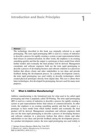
Obviously in the physical world, each layer must have a finite thickness to it and so
the resulting part will be an approximation of the original data, as illustrated by
Fig. 1.1. The thinner each layer is, the closer the final part will be to the original. All
commercialized AM machines to date use a layer-based approach, and the major
ways that they differ are in the materials that can be used, how the layers are
created, and how the layers are bonded to each other. Such differences will
determine factors like the accuracy of the final part plus its material properties
and mechanical properties. They will also determine factors like how quickly the
part can be made, how much post-processing is required, the size of the AM
machine used, and the overall cost of the machine and process.
This chapter will introduce the basic concepts of additive manufacturing and
describe a generic AM process from design to application. It will go on to discuss
the implications of AM on design and manufacturing and attempt to help in
understanding how it has changed the entire product development process. Since
AM is an increasingly important tool for product development, the chapter ends
with a discussion of some related tools in the product development process.
2 1 Introduction and Basic Principles](https://image.slidesharecdn.com/1-230308091212-68402451/85/1-Additive-manufacturing-pdf-24-320.jpg)
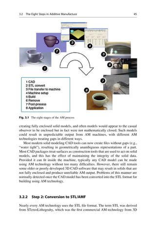
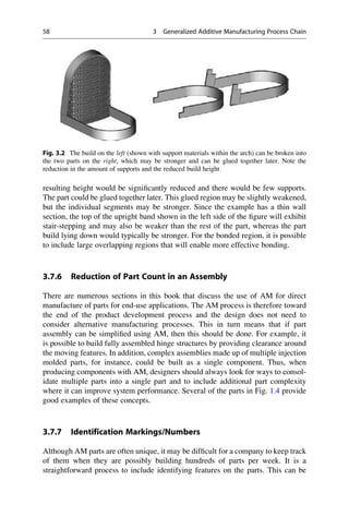
![1.3.6 Step 6: Removal
Once the AM machine has completed the build, the parts must be removed. This
may require interaction with the machine, which may have safety interlocks to
ensure for example that the operating temperatures are sufficiently low or that there
are no actively moving parts.
1.3.7 Step 7: Post-processing
Once removed from the machine, parts may require an amount of additional
cleaning up before they are ready for use. Parts may be weak at this stage or they
may have supporting features that must be removed. This therefore often requires
time and careful, experienced manual manipulation.
1.3.8 Step 8: Application
Parts may now be ready to be used. However, they may also require additional
treatment before they are acceptable for use. For example, they may require
priming and painting to give an acceptable surface texture and finish. Treatments
may be laborious and lengthy if the finishing requirements are very demanding.
They may also be required to be assembled together with other mechanical or
electronic components to form a final model or product.
While the numerous stages in the AM process have now been discussed, it is
important to realize that many AM machines require careful maintenance. Many
AM machines use fragile laser or printer technology that must be carefully moni-
tored and that should preferably not be used in a dirty or noisy environment. While
machines are generally designed to operate unattended, it is important to include
regular checks in the maintenance schedule, and that different technologies require
different levels of maintenance. It is also important to note that AM processes fall
outside of most materials and process standards; explaining the recent interest in the
ASTM F42 Technical Committee on Additive Manufacturing Technologies, which
is working to address and overcome this problem [1]. However, many machine
vendors recommend and provide test patterns that can be used periodically to
confirm that the machines are operating within acceptable limits.
In addition to the machinery, materials may also require careful handling. The
raw materials used in some AM processes have limited shelf-life and may also be
required to be kept in conditions that prevent them from unwanted chemical
reactions. Exposure to moisture, excess light, and other contaminants should also
be avoided. Most processes use materials that can be reused for more than one
build. However, it may be that reuse could degrade the properties if performed
many times over, and therefore a procedure for maintaining consistent material
quality through recycling should also be observed.
6 1 Introduction and Basic Principles](https://image.slidesharecdn.com/1-230308091212-68402451/85/1-Additive-manufacturing-pdf-28-320.jpg)
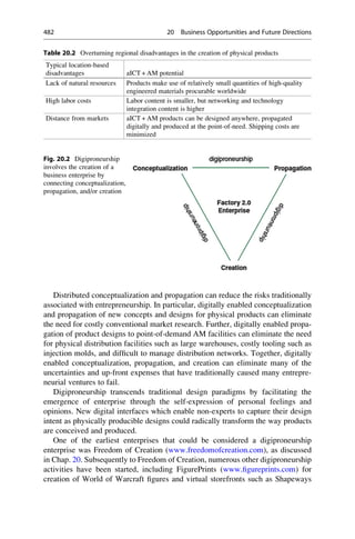
![1.4 Why Use the Term Additive Manufacturing?
By now, you should realize that the technology we are referring to is primarily the
use of additive processes, combining materials layer by layer. The term additive
manufacturing, or AM, seems to describe this quite well, but there are many other
terms which are in use. This section discusses other terms that have been used to
describe this technology as a way of explaining the overall purpose and benefits of
the technology for product development.
1.4.1 Automated Fabrication (Autofab)
This term was popularized by Marshall Burns in his book of the same name, which
was one of the first texts to cover this technology in the early 1990s [2]. The
emphasis here is on the use of automation to manufacture products, thus implying
the simplification or removal of manual tasks from the process. Computers and
microcontrollers are used to control the actuators and to monitor the system
variables. This term can also be used to describe other forms of Computer Numeri-
cal Controlled (CNC) machining centers since there is no direct reference as to how
parts are built or the number of stages it would take to build them, although Burns
does primarily focus on the technologies also covered by this book. Some key
technologies are however omitted since they arose after the book was written.
1.4.2 Freeform Fabrication or Solid Freeform Fabrication
The emphasis here is in the capability of the processes to fabricate complex
geometric shapes. Sometimes the advantage of these technologies is described in
terms of providing “complexity for free,” implying that it doesn’t particularly
matter what the shape of the input object actually is. A simple cube or cylinder
would take almost as much time and effort to fabricate within the machine as a
complex anatomical structure with the same enclosing volume. The reference to
“Freeform” relates to the independence of form from the manufacturing process.
This is very different from most conventional manufacturing processes that become
much more involved as the geometric complexity increases.
1.4.3 Additive Manufacturing or Layer-Based Manufacturing
These descriptions relate to the way the processes fabricate parts by adding material
in layers. This is in contrast to machining technology that removes, or subtracts
material from a block of raw material. It should be noted that some of the processes
are not purely additive, in that they may add material at one point but also use
subtractive processes at some stage as well. Currently, every commercial process
works in a layer-wise fashion. However, there is nothing to suggest that this is an
1.4 Why Use the Term Additive Manufacturing? 7](https://image.slidesharecdn.com/1-230308091212-68402451/85/1-Additive-manufacturing-pdf-29-320.jpg)
![essential approach to use and that future systems may add material in other ways
and yet still come under a broad classification that is appropriate to this text. A
slight variation on this, Additive Fabrication, is a term that was popularized by
Terry Wohlers, a well-known industry consultant in this field and who compiles a
widely regarded annual industry report on the state of this industry [3]. However,
many professionals prefer the term “manufacturing” to “fabrication” since “fabri-
cation” has some negative connotations that infer the part may still be a “prototype”
rather than a finished article. Additionally, in some regions of the world the term
fabrication is associated with sheet metal bending and related processes, and thus
professionals from these regions often object to the use of the word fabrication for
this industry. Additive manufacturing is, therefore, starting to become widely used,
and has also been adopted by Wohlers in his most recent publications and
presentations.
1.4.4 Stereolithography or 3D Printing
These two terms were initially used to describe specific machines.
Stereolithography (SL) was termed by the US company 3D Systems [4, 5] and
3D Printing (3DP) was widely used by researchers at MIT [6] who invented an
ink-jet printing-based technology. Both terms allude to the use of 2D processes
(lithography and printing) and extending them into the third dimension. Since most
people are very familiar with printing technology, the idea of printing a physical
three-dimensional object should make sense. Many consider that eventually the
term 3D Printing will become the most commonly used wording to describe AM
technologies. Recent media interest in the technology has proven this to be true and
the general public is much more likely to know the term 3D Printing than any other
term mentioned in this book.
1.4.5 Rapid Prototyping
Rapid prototyping was termed because of the process this technology was designed
to enhance or replace. Manufacturers and product developers used to find
prototyping a complex, tedious, and expensive process that often impeded the
developmental and creative phases during the introduction of a new product. RP
was found to significantly speed up this process and thus the term was adopted.
However, users and developers of this technology now realize that AM technology
can be used for much more than just prototyping.
Significant improvements in accuracy and material properties have seen this
technology catapulted into testing, tooling, manufacturing, and other realms that are
outside the “prototyping” definition. However, it can also be seen that most of the
other terms described above are also flawed in some way. One possibility is that
many will continue to use the term RP without specifically restricting it to the
manufacture of prototypes, much in the way that IBM makes things other than
8 1 Introduction and Basic Principles](https://image.slidesharecdn.com/1-230308091212-68402451/85/1-Additive-manufacturing-pdf-30-320.jpg)
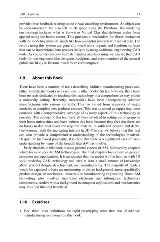
![set deposited the black material for the lines and the Objet name. Part c. is a section
of chain. Both parts b. and c. have working revolute joints that were fabricated using
clearances for the joints and dissolvable support structure. Part d. is a metal part that
was fabricated in a metal powder bed fusion machine using an electron beam as its
energy source (Chap. 5). The part is a model of a facial implant. Part e. was
fabricated in an Mcor Technologies sheet lamination machine that has ink-jet
printing capability for the multiple colors (Chap. 9). Parts f. and g. were fabricated
using material extrusion (Chap. 6). Part f. is a ratchet mechanism that was fabricated
in a single build in an industrial machine. Again, the working mechanism is achieved
through proper joint designs and dissolvable support structure. Part g. was fabricated
in a low-cost, personal machine (that one of the authors has at home). Parts h. and
i. were fabricated using polymer powder bed fusion. Part h. is the well-known “brain
gear” model of a three-dimensional gear train. When one gear is rotated, all other
gears rotate as well. Since parts fabricated in polymer PBF do not need supports,
working revolute and gear joints can be created by managing clearances and
removing the loose powder from the joint regions. Part i. is another conformal lattice
structure showing the shape complexity capability of AM technologies.
1.8 Other Related Technologies
The most common input method for AM technology is to accept a file converted
into the STL file format originally built within a conventional 3D CAD system.
There are, however, other ways in which the STL files can be generated and other
technologies that can be used in conjunction with AM technology. This section will
describe a few of these.
1.8.1 Reverse Engineering Technology
More and more models are being built from data generated using reverse engineer-
ing (RE) 3D imaging equipment and software. In this context, RE is the process of
capturing geometric data from another object. These data are usually initially
available in what is termed “point cloud” form, meaning an unconnected set of
points representing the object surfaces. These points need to be connected together
using RE software like Geomagic [7], which may also be used to combine point
clouds from different scans and to perform other functions like hole-filling and
smoothing. In many cases, the data will not be entirely complete. Samples may, for
example, need to be placed in a holding fixture and thus the surfaces adjacent to this
fixture may not be scanned. In addition, some surfaces may obscure others, like
with deep crevices and internal features; so that the representation may not turn out
exactly how the object is in reality. Recently there have been huge improvements in
scanning technology. An adapted handphone using its inbuilt camera can now
produce a high-quality 3D scan for just a few hundred dollars that even just a few
14 1 Introduction and Basic Principles](https://image.slidesharecdn.com/1-230308091212-68402451/85/1-Additive-manufacturing-pdf-36-320.jpg)
![years ago would have required an expensive laser-scanning or stereoscopic camera
system costing $100,000 or more.
Engineered objects would normally be scanned using laser-scanning or touch-
probe technology. Objects that have complex internal features or anatomical
models may make use of Computerized Tomography (CT), which was initially
developed for medical imaging but is also available for scanning industrially
produced objects. This technique essentially works in a similar way to AM, by
scanning layer by layer and using software to join these layers and identify the
surface boundaries. Boundaries from adjacent layers are then connected together to
form surfaces. The advantage of CT technology is that internal features can also be
generated. High-energy X-rays are used in industrial technology to create high-
resolution images of around 1 μm. Another approach that can help digitize objects
is the Capture Geometry Inside [8] technology that also works very much like a
reverse of AM technology, where 2D imaging is used to capture cross-sections of a
part as it is machined away layer by layer. Obviously this is a destructive approach
to geometry capture so it cannot be used for every type of product.
AM can be used to reproduce the articles that were scanned, which essentially
would form a kind of 3D facsimile (3D Fax) process. More likely, however, the data
will be modified and/or combined with other data to form complex, freeform
artifacts that are taking advantage of the “complexity for free” feature of the
technology. An example may be where individual patient data are combined with
an engineering design to form a customized medical implant. This is something that
will be discussed in much more detail later on in this book.
1.8.2 Computer-Aided Engineering
3D CAD is an extremely valuable resource for product design and development.
One major benefit to using software-based design is the ability to implement change
easily and cheaply. If we are able to keep the design primarily in a software format
for a larger proportion of the product development cycle, we can ensure that any
design changes are performed virtually on the software description rather than
physically on the product itself. The more we know about how the product is
going to perform before it is built, the more effective that product is going to
be. This is also the most cost-effective way to deal with product development. If
problems are only noticed after parts are physically manufactured, this can be very
costly. 3D CAD can make use of AM to help visualize and perform basic tests on
candidate designs prior to full-scale commitment to manufacturing. However, the
more complex and performance-related the design, the less likely we are to gain
sufficient insight using these methods. However, 3D CAD is also commonly linked
to other software packages, often using techniques like finite element method
(FEM) to calculate the mechanical properties of a design, collectively known as
Computer-Aided Engineering (CAE) software. Forces, dynamics, stresses, flow,
and other properties can be calculated to determine how well a design will perform
under certain conditions. While such software cannot easily predict the exact
1.8 Other Related Technologies 15](https://image.slidesharecdn.com/1-230308091212-68402451/85/1-Additive-manufacturing-pdf-37-320.jpg)
![behavior of a part, for analysis of critical parts a combination of CAE, backed up
with AM-based experimental analysis, may be a useful solution. Further, with the
advent of Direct Digital Manufacture, where AM can be used to directly produce
final products, there is an increasing need for CAE tools to evaluate how these parts
would perform prior to AM so that we can build these products right first time as a
form of Design for Additive Manufacturing (D for AM).
1.8.3 Haptic-Based CAD
3D CAD systems are generally built on the principle that models are constructed
from basic geometric shapes that are then combined in different ways to make more
complex forms. This works very well for the engineered products we are familiar
with, but may not be so effective for more unusual designs. Many consumer
products are developed from ideas generated by artists and designers rather than
engineers. We also note that AM has provided a mechanism for greater freedom of
expression. AM is in fact now becoming a popular tool for artists and sculptors,
like, for example, Bathsheba Grossman [9] who takes advantage of the geometric
freedom to create visually exciting sculptures. One problem we face today is that
some computer-based design tools constrain or restrict the creative processes and
that there is scope for a CAD system that provides greater freedom. Haptic-based
CAD modeling systems like the experimental system shown in Fig. 1.5 [10], work
in a similar way to the commercially available Freeform [11] modeling system to
provide a design environment that is more intuitive than other standard CAD
systems. They often use a robotic haptic feedback device called the Phantom to
Fig. 1.5 Freeform modeling system
16 1 Introduction and Basic Principles](https://image.slidesharecdn.com/1-230308091212-68402451/85/1-Additive-manufacturing-pdf-38-320.jpg)
![greater functionality and embrace a wider range of applications beyond the initial
intention of just prototyping.
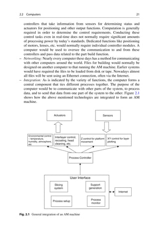
2.2 Computers
Like many other technologies, AM came about as a result of the invention of the
computer. However, there was little indication that the first computers built in the
1940s (like the Zuse Z3 [1], ENIAC [2] and EDSAC [3] computers) would change
lives in the way that they so obviously have. Inventions like the thermionic valve,
transistor, and microchip made it possible for computers to become faster, smaller,
and cheaper with greater functionality. This development has been so quick that
even Bill Gates of Microsoft was caught off-guard when he thought in 1981 that
640 kb of memory would be sufficient for any Windows-based computer. In 1989,
he admitted his error when addressing the University of Waterloo Computer
Science Club [4]. Similarly in 1977, Ken Olsen of Digital Electronics Corp.
(DEC) stated that there would never be any reason for people to have computers
in their homes when he addressed the World Future Society in Boston [5]. That
remarkable misjudgment may have caused Olsen to lose his job not long
afterwards.
One key to the development of computers as serviceable tools lies in their ability
to perform tasks in real-time. In the early days, serious computational tasks took
many hours or even days to prepare, run, and complete. This served as a hindrance
to everyday computer use and it is only since it was shown that tasks can be
completed in real-time that computers have been accepted as everyday items rather
than just for academics or big business. This has included the ability to display
results not just numerically but graphically as well. For this we owe a debt of thanks
at least in part to the gaming industry, which has pioneered many developments in
graphics technology with the aim to display more detailed and more “realistic”
images to enhance the gaming experience.
AM takes full advantage of many of the important features of computer technol-
ogy, both directly (in the AM machines themselves) and indirectly (within the
supporting technology), including:
– Processing power: Part data files can be very large and require a reasonable
amount of processing power to manipulate while setting up the machine and
when slicing the data before building. Earlier machines would have had diffi-
culty handling large CAD data files.
– Graphics capability: AM machine operation does not require a big graphics
engine except to see the file while positioning within the virtual machine space.
However, all machines benefit from a good graphical user interface (GUI) that
can make the machine easier to set up, operate, and maintain.
– Machine control: AM technology requires precise positioning of equipment in a
similar way to a Computer Numerical Controlled (CNC) machining center, or
even a high-end photocopy machine or laser printer. Such equipment requires
20 2 Development of Additive Manufacturing Technology](https://image.slidesharecdn.com/1-230308091212-68402451/85/1-Additive-manufacturing-pdf-42-320.jpg)


![in improvements in the way CAD data is presented, manipulated, and stored. Most
CAD systems these days utilize Non-Uniform Rational Basis-Splines, or NURBS
[6]. NURBS are an excellent way of precisely defining the curves and surfaces that
correspond to the outer shell of a CAD model. Since model definitions can include
free form surfaces as well as simple geometric shapes, the representation must
accommodate this and splines are complex enough to represent such shapes without
making the files too large and unwieldy. They are also easy to manipulate to modify
the resulting shape.
CAD technology has rapidly improved along the following lines:
– Realism: With lighting and shading effects, ray tracing and other photorealistic
imaging techniques, it is becoming possible to generate images of the CAD
models that are difficult to distinguish from actual photographs. In some ways,
this reduces the requirements on AM models for visualization purposes.
– Usability and user interface: Early CAD software required the input of text-
based instructions through a dialog box. Development of Windows-based GUIs
has led to graphics-based dialogs and even direct manipulation of models within
virtual 3D environments. Instructions are issued through the use of drop-down
menu systems and context-related commands. To suit different user preferences
and styles, it is often possible to execute the same instruction in different ways.
Keyboards are still necessary for input of specific measurements, but the usabil-
ity of CAD systems has improved dramatically. There is still some way to go to
make CAD systems available to those without engineering knowledge or with-
out training, however.
– Engineering content: Since CAD is almost an essential part of a modern
engineer’s training, it is vital that the software includes as much engineering
content as possible. With solid modeling CAD it is possible to calculate the
volumes and masses of models, investigate fits and clearances according to
tolerance variations, and to export files with mesh data for FEA. FEA is often
even possible without having to leave the CAD system.
– Speed: As mentioned previously, the use of NURBS assists in optimizing CAD
data manipulation. CAD systems are constantly being optimized in various
ways, mainly by exploiting the hardware developments of computers.
– Accuracy: If high tolerances are expected for a design then it is important that
calculations are precise. High precision can make heavy demands on processing
time and memory.
– Complexity: All of the above characteristics can lead to extremely complex
systems. It is a challenge to software vendors to incorporate these features
without making them unwieldy and unworkable.
– Usability: Recent developments in CAD technology have focused on making the
systems available to a wider range of users. In particular the aim has been to
allow untrained users to be able to design complex geometry parts for them-
selves. There are now 3D solid modeling CAD systems that run entirely within a
web browser with similar capabilities of workstation systems of only
10 years ago.
24 2 Development of Additive Manufacturing Technology](https://image.slidesharecdn.com/1-230308091212-68402451/85/1-Additive-manufacturing-pdf-46-320.jpg)
![Many CAD software vendors are focusing on producing highly integrated design
environments that allow designers to work as teams and to share designs across
different platforms and for different departments. Industrial designers must work
with sales and marketing, engineering designers, analysts, manufacturing
engineers, and many other branches of an organization to bring a design to fruition
as a product. Such branches may even be in different regions of the world and may
be part of the same organization or acting as subcontractors. The Internet must
therefore also be integrated with these software systems, with appropriate measures
for fast and accurate transmission and protection of intellectual property.
It is quite possible to directly manipulate the CAD file to generate the slice data
that will drive an AM machine, and this is commonly referred to as direct slicing
[7]. However, this would mean every CAD system must have a direct slicing
algorithm that would have to be compatible with all the different types of AM
technology. Alternatively, each AM system vendor would have to write a routine
for every CAD system. Both of these approaches are impractical. The solution is to
use a generic format that is specific to the technology. This generic format was
developed by 3D Systems, USA, who was the first company to commercialize AM
technology and called the file format “STL” after their stereolithography technol-
ogy (an example of which is shown in Fig. 2.2).
The STL file format was made public domain to allow all CAD vendors to access it
easily and hopefully integrate it into their systems. This strategy has been successful
and STL is now a standard output for nearly all solid modeling CAD systems and has
also been adopted by AM system vendors [8]. STL uses triangles to describe the
surfaces to be built. Each triangle is described as three points and a facet normal vector
indicating the outward side of the triangle, in a manner similar to the following:
facet normal 4.470293E 02 7.003503E 01 7.123981E-01
outer loop
vertex 2.812284E + 00 2.298693E + 01 0.000000E + 00
vertex 2.812284E + 00 2.296699E + 01 1.960784E 02
vertex 3.124760E + 00 2.296699E + 01 0.000000E + 00
endloop
endfacet
Fig. 2.2 A CAD model on the left converted into STL format on the right
2.3 Computer-Aided Design Technology 25](https://image.slidesharecdn.com/1-230308091212-68402451/85/1-Additive-manufacturing-pdf-47-320.jpg)
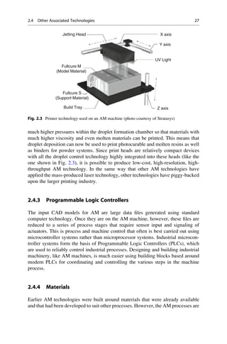
![somewhat unique and these original materials were far from ideal for these new
applications. For example, the early photocurable resins resulted in models that
were brittle and that warped easily. Powders used in laser-based powder bed fusion
processes degraded quickly within the machine and many of the materials used
resulted in parts that were quite weak. As we came to understand the technology
better, materials were developed specifically to suit AM processes. Materials have
been tuned to suit more closely the operating parameters of the different processes
and to provide better output parts. As a result, parts are now much more accurate,
stronger, and longer lasting and it is even possible to process metals with some AM
technologies. In turn, these new materials have resulted in the processes being tuned
to produce higher temperature materials, smaller feature sizes, and faster
throughput.
2.4.5 Computer Numerically Controlled Machining
One of the reasons AM technology was originally developed was because CNC
technology was not able to produce satisfactory output within the required time
frames. CNC machining was slow, cumbersome, and difficult to operate. AM
technology on the other hand was quite easy to set up with quick results, but had
poor accuracy and limited material capability. As improvements in AM
technologies came about, vendors of CNC machining technology realized that
there was now growing competition. CNC machining has dramatically improved,
just as AM technologies have matured. It could be argued that high-speed CNC
would have developed anyway, but some have argued that the perceived threat from
AM technology caused CNC machining vendors to rethink how their machines
were made. The development of hybrid prototyping technologies, such as Space
Puzzle Molding that use both high-speed machining and additive techniques for
making large, complex and durable molds and components, as shown in Fig. 2.4
[9], illustrate how the two can be used interchangeably to take advantage of the
benefits of both technologies. For geometries that can be machined using a single
set-up orientation, CNC machining is often the fastest, most cost-effective method.
For parts with complex geometries or parts which require a large proportion of the
overall material volume to be machined away as scrap, AM can be used to more
quickly and economically produce the part than when using CNC.
2.5 The Use of Layers
A key enabling principle of AM part manufacture is the use of layers as finite 2D
cross-sections of the 3D model. Almost every AM technology builds parts using
layers of material added together; and certainly all commercial systems work that
way, primarily due to the simplification of building 3D objects. Using 2D
representations to represent cross-sections of a more complex 3D feature has
been common in many applications outside AM. The most obvious example of
28 2 Development of Additive Manufacturing Technology](https://image.slidesharecdn.com/1-230308091212-68402451/85/1-Additive-manufacturing-pdf-50-320.jpg)
![this is how cartographers use a line of constant height to represent hills and other
geographical reliefs. These contour lines, or iso-heights, can be used as plates that
can be stacked to form representations of geographical regions. The gaps between
these 2D cross-sections cannot be precisely represented and are therefore
approximated, or interpolated, in the form of continuity curves connecting these
layers. Such techniques can also be used to provide a 3D representation of other
physical properties, like isobars or isotherms on weather maps.
Architects have also used such methods to represent landscapes of actual or
planned areas, like that used by an architect firm in Fig. 2.5 [10]. The concept is
particularly logical to manufacturers of buildings who also use an additive
Fig. 2.4 Space puzzle
molding, where molds are
constructed in segments for
fast and easy fabrication and
assembly (photo courtesy of
Protoform, Germany)
Fig. 2.5 An architectural
landscape model, illustrating
the use of layers (photo
courtesy of LiD)
2.5 The Use of Layers 29](https://image.slidesharecdn.com/1-230308091212-68402451/85/1-Additive-manufacturing-pdf-51-320.jpg)
![approach, albeit not using layers. Consider how the pyramids in Egypt and in South
America were created. Notwithstanding how they were fabricated, it’s clear that
they were created using a layered approach, adding material as they went.
2.6 Classification of AM Processes
There are numerous ways to classify AM technologies. A popular approach is to
classify according to baseline technology, like whether the process uses lasers,
printer technology, extrusion technology, etc. [11, 12]. Another approach is to
collect processes together according to the type of raw material input [13]. The
problem with these classification methods is that some processes get lumped
together in what seems to be odd combinations (like Selective Laser Sintering
(SLS) being grouped together with 3D Printing) or that some processes that may
appear to produce similar results end up being separated (like Stereolithography
and material jetting with photopolymers). It is probably inappropriate, therefore, to
use a single classification approach.
An excellent and comprehensive classification method is described by Pham
[14], which uses a two-dimensional classification method as shown in Fig. 2.6. The
first dimension relates to the method by which the layers are constructed. Earlier
technologies used a single point source to draw across the surface of the base
material. Later systems increased the number of sources to increase the throughput,
which was made possible with the use of droplet deposition technology, for
example, which can be constructed into a one dimensional array of deposition
1D Channel 2x1D Channels 2D Channel
Array of 1D
Channels
SLA (3D Sys)
Dual beam
SLA (3D Sys)
Objet
DPS
Envisiontech
MicroTEC
3D Printing
ThermoJet
LST (EOS)
Solido
PLT (KIRA)
FDM, Solidscape
SLS (3D Sys),
LST (EOS), LENS
Phenix, SDM
Liquid
Polymer
Discrete
Particles
Molten
Mat.
Solid
Sheets
X
X
X
Y
X1
Y1
X2
Y2
Y
Fig. 2.6 Layered manufacturing (LM) processes as classified by Pham (note that this diagram has
been amended to include some recent AM technologies)
30 2 Development of Additive Manufacturing Technology](https://image.slidesharecdn.com/1-230308091212-68402451/85/1-Additive-manufacturing-pdf-52-320.jpg)
![heads. Further throughput improvements are possible with the use of 2D array
technology using the likes of Digital Micro-mirror Devices (DMDs) and high-
resolution display technology, capable of exposing an entire surface in a single
pass. However, just using this classification results in the previously mentioned
anomalies where numerous dissimilar processes are grouped together. This is
solved by introducing a second dimension of raw material to the classification.
Pham uses four separate material classifications; liquid polymer, discrete particles,
molten material, and laminated sheets. Some more exotic systems mentioned in this
book may not fit directly into this classification. An example is the possible
deposition of composite material using an extrusion-based technology. This fits
well as a 1D channel but the material is not explicitly listed, although it could be
argued that the composite is extruded as a molten material. Furthermore, future
systems may be developed that use 3D holography to project and fabricate complete
objects in a single pass. As with many classifications, there can sometimes be
processes or systems that lie outside them. If there are sufficient systems to warrant
an extension to this classification, then it should not be a problem.
It should be noted that, in particular 1D and 2 1D channel systems combine
both vector- and raster-based scanning methods. Often, the outline of a layer is
traced first before being filled in with regular or irregular scanning patterns. The
outline is generally referred to as vector scanned while the fill pattern can often be
generalized as a raster pattern. The array methods tend not to separate the outline
and the fill.
Most AM technology started using a 1D channel approach, although one of the
earliest and now obsolete technologies, Solid Ground Curing from Cubital, used
liquid photopolymers and essentially (although perhaps arguably) a 2D channel
method. As technology developed, so more of the boxes in the classification array
began to be filled. The empty boxes in this array may serve as a guide to researchers
and developers for further technological advances. Most of the 1D array methods
use at least 2 1D lines. This is similar to conventional 2D printing where each line
deposits a different material in different locations within a layer. The recent Connex
process using the Polyjet technology from Stratasys is a good example of this where
it is now possible to create parts with different material properties in a single step
using this approach. Color 3D Printing is possible using multiple 1D arrays with ink
or separately colored material in each. Note however that the part coloration in the
sheet laminating Mcor process [15] is separated from the layer formation process,
which is why it is defined as a 1D channel approach.
2.6.1 Liquid Polymer Systems
As can be seen from Fig. 2.5 liquid polymers appear to be a popular material. The
first commercial system was the 3D Systems Stereolithography process based on
liquid photopolymers. A large portion of systems in use today are, in fact, not just
liquid polymer systems but more specifically liquid photopolymer systems. How-
ever, this classification should not be restricted to just photopolymers, since a
2.6 Classification of AM Processes 31](https://image.slidesharecdn.com/1-230308091212-68402451/85/1-Additive-manufacturing-pdf-53-320.jpg)
![number of experimental systems are using hydrogels that would also fit into this
category. Furthermore, the Fab@home system developed at Cornell University in
the USA and the open source RepRap systems originating from Bath University in
the UK also use liquid polymers with curing techniques other than UV or other
wavelength optical curing methods [16, 17].
Using this material and a 1D channel or 2 1D channel scanning method, the
best option is to use a laser like in the Stereolithography process. Droplet deposition
of polymers using an array of 1D channels can simplify the curing process to a
floodlight (for photopolymers) or similar method. This approach is used with
machines made by the Israeli company Objet (now part of Stratasys) who uses
printer technology to print fine droplets of photopolymer “ink” [18]. One unique
feature of the Objet system is the ability to vary the material properties within a
single part. Parts can for example have soft-feel, rubber-like features combined
with more solid resins to achieve a result similar to an overmolding effect.
Controlling the area to be exposed using DMDs or other high-resolution display
technology obviates the need for any scanning at all, thus increasing throughput and
reducing the number of moving parts. DMDs are generally applied to micron-scale
additive approaches, like those used by Microtec in Germany [19]. For normal-
scale systems Envisiontec uses high-resolution DMD displays to cure photopoly-
mer resin in their low-cost AM machines. The 3D Systems V-Flash process is also a
variation on this approach, exposing thin sheets of polymer spread onto a build
surface.
2.6.2 Discrete Particle Systems
Discrete particles are normally powders that are generally graded into a relatively
uniform particle size and shape and narrow size distribution. The finer the particles
the better, but there will be problems if the dimensions get too small in terms of
controlling the distribution and dispersion. Again, the conventional 1D channel
approach is to use a laser, this time to produce thermal energy in a controlled
manner and, therefore, raise the temperature sufficiently to melt the powder.
Polymer powders must therefore exhibit thermoplastic behavior so that they can
be melted and re-melted to permit bonding of one layer to another. There are a wide
variety of such systems that generally differ in terms of the material that can be
processed. The two main polymer-based systems commercially available are the
SLS technology marketed by 3D Systems [20] and the EOSint processes developed
by the German company EOS [21].
Application of printer technology to powder beds resulted in the (original) 3D
Printing (3DP) process. This technique was developed by researchers at MIT in the
USA [22]. Droplet printing technology is used to print a binder, or glue, onto a
powder bed. The glue sticks the powder particles together to form a 3D structure.
This basic technique has been developed for different applications dependent on the
type of powder and binder combination. The most successful approaches use
low-cost, starch- and plaster-based powders with inexpensive glues, as
32 2 Development of Additive Manufacturing Technology](https://image.slidesharecdn.com/1-230308091212-68402451/85/1-Additive-manufacturing-pdf-54-320.jpg)
![commercialized by ZCorp, USA [23], which is now part of 3D Systems. Ceramic
powders and appropriate binders as similarly used in the Direct Shell Production
Casting (DSPC) process used by Soligen [24] as part of a service to create shells for
casting of metal parts. Alternatively, if the binder were to contain an amount of
drug, 3DP can be used to create controlled delivery-rate drugs like in the process
developed by the US company Therics. Neither of these last two processes has
proven to be as successful as that licensed by ZCorp/3D Systems. One particular
advantage of the former ZCorp technology is that the binders can be jetted from
multinozzle print heads. Binders coming from different nozzles can be different
and, therefore, subtle variations can be incorporated into the resulting part. The
most obvious of these is the color that can be incorporated into parts.
2.6.3 Molten Material Systems
Molten material systems are characterized by a pre-heating chamber that raises the
material temperature to melting point so that it can flow through a delivery system.
The most well-known method for doing this is the Fused Deposition Modeling
(FDM) material extrusion technology developed by the US company Stratasys
[25]. This approach extrudes the material through a nozzle in a controlled manner.
Two extrusion heads are often used so that support structures can be fabricated from
a different material to facilitate part cleanup and removal. It should be noted that
there are now a huge number of variants of this technology due to the lapse of key
FDM patents, with the number of companies making these perhaps even into three
figures. This competition has driven the price of these machines down to such a
level that individual buyers can afford to have their own machines at home.
Printer technology has also been adapted to suit this material delivery approach.
One technique, developed initially as the Sanders prototyping machine, that later
became Solidscape, USA [26] and which is now part of Stratasys, is a 1D channel
system. A single jet piezoelectric deposition head lays down wax material. Another
head lays down a second wax material with a lower melting temperature that is used
for support structures. The droplets from these print heads are very small so the
resulting parts are fine in detail. To further maintain the part precision, a planar
cutting process is used to level each layer once the printing has been completed.
Supports are removed by inserting the complete part into a temperature-controlled
bath that melts the support material away, leaving the part material intact. The use
of wax along with the precision of Solidscape machines makes this approach ideal
for precision casting applications like jewelry, medical devices, and dental castings.
Few machines are sold outside of these niche areas.
The 1D channel approach, however, is very slow in comparison with other
methods and applying a parallel element does significantly improve throughput.
The Thermojet technology from 3D Systems also deposits a wax material through
droplet-based printing heads. The use of parallel print heads as an array of 1D
channels effectively multiplies the deposition rate. The Thermojet approach, how-
ever, is not widely used because wax materials are difficult and fragile when
2.6 Classification of AM Processes 33](https://image.slidesharecdn.com/1-230308091212-68402451/85/1-Additive-manufacturing-pdf-55-320.jpg)
![handled. Thermojet machines are no longer being made, although existing
machines are commonly used for investment casting patterns.
2.6.4 Solid Sheet Systems
One of the earliest AM technologies was the Laminated Object Manufacturing
(LOM) system from Helisys, USA. This technology used a laser to cut out profiles
from sheet paper, supplied from a continuous roll, which formed the layers of the
final part. Layers were bonded together using a heat-activated resin that was coated
on one surface of the paper. Once all the layers were bonded together the result was
very much like a wooden block. A hatch pattern cut into the excess material allowed
the user to separate away waste material and reveal the part.
A similar approach was used by the Japanese company Kira, in their Solid
Center machine [27], and by the Israeli company Solidimension with their Solido
machine. The major difference is that both these machines cut out the part profile
using a blade similar to those found in vinyl sign-making machines, driven using a
2D plotter drive. The Kira machine used a heat-activated adhesive applied using
laser printing technology to bond the paper layers together. Both the Solido and
Kira machines have been discontinued for reasons like poor reliability material
wastage and the need for excessive amounts of manual post-processing. Recently,
however, Mcor Technologies have produced a modern version of this technology,
using low-cost color printing to make it possible to laminate color parts in a single
process [28].
2.6.5 New AM Classification Schemes
In this book, we use a version of Pham’s classification introduced in Fig. 2.6.
Instead of using the 1D and 2 1D channel terminology, we will typically use the
terminology “point” or “point-wise” systems. For arrays of 1D channels, such as
when using ink-jet print heads, we refer to this as “line” processing. 2D Channel
technologies will be referred to as “layer” processing. Last, although no current
commercialized processes are capable of this, holographic-like techniques are
considered “volume” processing.
The technology-specific descriptions starting in Chap. 4 are based, in part, upon
a separation of technologies into groups where processes which use a common type
of machine architecture and similar materials transformation physics are grouped
together. This grouping is a refinement of an approach introduced by Stucker and
Janaki Ram in the CRC Materials Processing Handbook [29]. In this grouping
scheme, for example, processes which use a common machine architecture devel-
oped for stacking layers of powdered material and a materials transformation
mechanism using heat to fuse those powders together are all discussed in the
Powder Bed Fusion chapter. These are grouped together even though these pro-
cesses encompass polymer, metal, ceramic, and composite materials, multiple types
34 2 Development of Additive Manufacturing Technology](https://image.slidesharecdn.com/1-230308091212-68402451/85/1-Additive-manufacturing-pdf-56-320.jpg)
![of energy sources (e.g., lasers, and infrared heaters), and point-wise and layer
processing approaches. Using this classification scheme, all AM processes fall
into one of seven categories. An understanding of these seven categories should
enable a person familiar with the concepts introduced in this book to quickly grasp
and understand an unfamiliar AM process by comparing its similarities, benefits,
drawbacks, and processing characteristics to the other processes in the grouping
into which it falls.
This classification scheme from the first edition of this textbook had an impor-
tant impact on the development and adoption of ASTM/ISO standard terminology.
The authors were involved in these consensus standards activities and we have
agreed to adopt the modified terminology from ASTM F42 and ISO TC 261 in the
second edition. Of course, in the future, we will continue to support the ASTM/ISO
standardization efforts and keep the textbook up to date.
The seven process categories are presented here. Chapters 4–10 cover each one
in detail:
• Vat photopolymerization: processes that utilize a liquid photopolymer that is
contained in a vat and processed by selectively delivering energy to cure specific
regions of a part cross-section.
• Powder bed fusion: processes that utilize a container filled with powder that is
processed selectively using an energy source, most commonly a scanning laser
or electron beam.
• Material extrusion: processes that deposit a material by extruding it through a
nozzle, typically while scanning the nozzle in a pattern that produces a part
cross-section.
• Material jetting: ink-jet printing processes.
• Binder jetting: processes where a binder is printed into a powder bed in order to
form part cross-sections.
• Sheet lamination: processes that deposit a layer of material at a time, where the
material is in sheet form.
• Directed energy deposition: processes that simultaneously deposit a material
(usually powder or wire) and provide energy to process that material through a
single deposition device.
2.7 Metal Systems
One of the most important recent developments in AM has been the proliferation of
direct metal processes. Machines like the EOSint-M [21] and Laser-Engineered Net
Shaping (LENS) have been around for a number of years [30, 31]. Recent additions
from other companies and improvements in laser technology, machine accuracy,
speed, and cost have opened up this market.
Most direct metal systems work using a point-wise method and nearly all of
them utilize metal powders as input. The main exception to this approach is the
sheet lamination processes, particularly the Ultrasonic Consolidation process from
2.7 Metal Systems 35](https://image.slidesharecdn.com/1-230308091212-68402451/85/1-Additive-manufacturing-pdf-57-320.jpg)
![the Solidica, USA, which uses sheet metal laminates that are ultrasonically welded
together [32]. Of the powder systems, almost every newer machine uses a powder
spreading approach similar to the SLS process, followed by melting using an energy
beam. This energy is normally a high-power laser, except in the case of the Electron
Beam Melting (EBM) process by the Swedish company Arcam [33]. Another
approach is the LENS powder delivery system used by Optomec [31]. This machine
employs powder delivery through a nozzle placed above the part. The powder is
melted where the material converges with the laser and the substrate. This approach
allows the process to be used to add material to an existing part, which means it can
be used for repair of expensive metal components that may have been damaged,
like chipped turbine blades and injection mold tool inserts.
2.8 Hybrid Systems
Some of the machines described above are, in fact, hybrid additive/subtractive
processes rather than purely additive. Including a subtractive component can assist
in making the process more precise. An example is the use of planar milling at the
end of each additive layer in the Sanders and Objet machines. This stage makes for
a smooth planar surface onto which the next layer can be added, negating cumula-
tive effects from errors in droplet deposition height.
It should be noted that when subtractive methods are used, waste will be
generated. Machining processes require removal of material that in general cannot
easily be recycled. Similarly, many additive processes require the use of support
structures and these too must be removed or “subtracted.”
It can be said that with the Objet process, for instance, the additive element is
dominant and that the subtractive component is important but relatively insignifi-
cant. There have been a number of attempts to merge subtractive and additive
technologies together where the subtractive component is the dominant element.
An excellent example of this is the Stratoconception approach [34], where the
original CAD models are divided into thick machinable layers. Once these layers
are machined, they are bonded together to form the complete solid part. This
approach works very well for very large parts that may have features that would
be difficult to machine using a multi-axis machining center due to the accessibility
of the tool. This approach can be applied to foam and wood-based materials or to
metals. For structural components it is important to consider the bonding methods.
For high strength metal parts diffusion bonding may be an alternative.
A lower cost solution that works in a similar way is Subtractive RP (SRP) from
Roland [35], who is also famous for plotter technology. SRP makes use of Roland
desktop milling machines to machine sheets of material that can be sandwiched
together, similar to Stratoconception. The key is to use the exterior material as a
frame that can be used to register each slice to others and to hold the part in place.
With this method not all the material is machined away and a web of connecting
spars are used to maintain this registration.
36 2 Development of Additive Manufacturing Technology](https://image.slidesharecdn.com/1-230308091212-68402451/85/1-Additive-manufacturing-pdf-58-320.jpg)
![Another variation of this method that was never commercialized was Shaped
Deposition Manufacturing (SDM), developed mainly at Stanford and Carnegie-
Mellon Universities in the USA [36]. With SDM, the geometry of the part is
devolved into a sequence of easier to manufacture parts that can in some way be
combined together. A decision is made concerning whether each subpart should be
manufactured using additive or subtractive technology dependent on such factors as
the accuracy, material, geometrical features, functional requirements, etc. Further-
more, parts can be made from multiple materials, combined together using a variety
of processes, including the use of plastics, metals and even ceramics. Some of the
materials can also be used in a sacrificial way to create cavities and clearances.
Additionally, the “layers” are not necessarily planar, nor constant in thickness. Such
a system would be unwieldy and difficult to realize commercially, but the ideas
generated during this research have influenced many studies and systems thereafter.
In this book, for technologies where both additive and subtractive approaches
are used, these technologies are discussed in the chapter where their additive
approach best fits.
2.9 Milestones in AM Development
We can look at the historical development of AM in a variety of different ways. The
origins may be difficult to properly define and there was certainly quite a lot of
activity in the 1950s and 1960s, but development of the associated technology
(computers, lasers, controllers, etc.) caught up with the concept in the early 1980s.
Interestingly, parallel patents were filed in 1984 in Japan (Murutani), France (Andre
et al.) and in the USA (Masters in July and Hull in August). All of these patents
described a similar concept of fabricating a 3D object by selectively adding
material layer by layer. While earlier work in Japan is quite well-documented,
proving that this concept could be realized, it was the patent by Charles Hull that is
generally recognized as the most influential since it gave rise to 3D Systems. This
was the first company to commercialize AM technology with the Stereolithography
apparatus (Fig. 2.7).
Further patents came along in 1986, resulting in three more companies, Helisys
(Laminated Object Manufacture or LOM), Cubital (with Solid Ground Curing,
SGC), and DTM with their SLS process. It is interesting to note neither Helisys
nor Cubital exist anymore, and only SLS remains as a commercial process with
DTM merging with 3D Systems in 2001. In 1989, Scott Crump patented the FDM
process, forming the Stratasys Company. Also in 1989 a group from MIT patented
the 3D Printing (3DP) process. These processes from 1989 are heavily used today,
with FDM variants currently being the most successful. Rather than forming a
company, the MIT group licensed the 3DP technology to a number of different
companies, who applied it in different ways to form the basis for different
applications of their AM technology. The most successful of these was ZCorp,
which focused mainly on low-cost technology.
2.9 Milestones in AM Development 37](https://image.slidesharecdn.com/1-230308091212-68402451/85/1-Additive-manufacturing-pdf-59-320.jpg)
![2.10 AM Around the World
As was already mentioned, early patents were filed in Europe (France), USA, and
Asia (Japan) almost simultaneously. In early years, most pioneering and commer-
cially successful systems came out of the USA. Companies like Stratasys, 3D
Systems, and ZCorp have spearheaded the way forward. These companies have
generally strengthened over the years, but most new companies have come from
outside the USA.
In Europe, the primary company with a world-wide impact in AM is EOS,
Germany. EOS stopped making SL machines following settlement of disputes
with 3D Systems but continues to make powder bed fusion systems which use
lasers to melt polymers, binder-coated sand, and metals. Companies from France,
The Netherlands, Sweden, and other parts of Europe are smaller, but are competi-
tive in their respective marketplaces. Examples of these companies include Phenix
[37] (now part of 3D Systems), Arcam, Strataconception, and Materialise. The last
of these, Materialise from Belgium [38], has seen considerable success in develop-
ing software tools to support AM technology.
In the early 1980s and 1990s, a number of Japanese companies focused on AM
technology. This included startup companies like Autostrade (which no longer
appears to be operating). Large companies like Sony and Kira, who established
subsidiaries to build AM technology, also became involved. Much of the Japanese
technology was based around the photopolymer curing processes. With 3D Systems
dominant in much of the rest of the world, these Japanese companies struggled to
find market and many of them failed to become commercially viable, even though
their technology showed some initial promise. Some of this demise may have
resulted in the unusually slow uptake of CAD technology within Japanese industry
in general. Although the Japanese company CMET [39] still seems to be doing
quite well, you will likely find more non-Japanese made machines in Japan than
home-grown ones. There is some indication however that this is starting to change.
AM technology has also been developed in other parts of Asia, most notably in
Korea and China. Korean AM companies are relatively new and it remains to be
seen whether they will make an impact. There are, however, quite a few Chinese
manufacturers who have been active for a number of years. Patent conflicts with the
earlier USA, Japanese, and European designs have meant that not many of these
machines can be found outside of China. Earlier Chinese machines were also
thought to be of questionable quality, but more recent machines have markedly
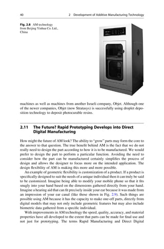
improved performance (like the machine shown in Fig. 2.8). Chinese machines
primarily reflect the SL, FDM, and SLS technologies found elsewhere in the world.
A particular country of interest in terms of AM technology development is
Israel. One of the earliest AM machines was developed by the Israeli company
Cubital. Although this technology was not a commercial success, in spite of early
installations around the world, they demonstrated a number of innovations not
found in other machines, including layer processing through a mask, removable
secondary support materials and milling after each layer to maintain a constant
layer thickness. Some of the concepts used in Cubital can be found in Sanders
2.10 AM Around the World 39](https://image.slidesharecdn.com/1-230308091212-68402451/85/1-Additive-manufacturing-pdf-61-320.jpg)
![Systems in the 1990s. Considered a de facto standard, STL is a simple way of
describing a CAD model in terms of its geometry alone. It works by removing any
construction data, modeling history, etc., and approximating the surfaces of the
model with a series of triangular facets. The minimum size of these triangles can be
set within most CAD software and the objective is to ensure the models created do
not show any obvious triangles on the surface. The triangle size is in fact calculated
in terms of the minimum distance between the plane represented by the triangle and
the surface it is supposed to represent. In other words, a basic rule of thumb is to
ensure that the minimum triangle offset is smaller than the resolution of the AM
machine. The process of converting to STL is automatic within most CAD systems,
but there is a possibility of errors occurring during this phase. There have therefore
been a number of software tools developed to detect such errors and to rectify them
if possible.
STL files are an unordered collection of triangle vertices and surface normal
vectors. As such, an STL file has no units, color, material, or other feature
information. These limitations of an STL file have led to the recent adoption of a
new “AMF” file format. This format is now an international ASTM/ISO standard
format which extends the STL format to include dimensions, color, material, and
many other useful features. As of the writing of this book, several major CAD
companies and AM hardware vendors had publically announced that they will be
supporting AMF in their next generation software. Thus, although the term STL is
used throughout the remainder of this textbook, the AMF file could be simply
substituted wherever STL appears, as the AMF format has all of the benefits of the
STL file format with many fewer limitations.
STL file repair software, like the MAGICS software from the Belgian company
Materialise [1], is used when there are problems with the STL file that may prevent
the part from being built correctly. With complex geometries, it may be difficult for
a human to detect such problems when inspecting the CAD or the subsequently
generated STL data. If the errors are small then they may even go unnoticed until
after the part has been built. Such software may therefore be applied as a checking
stage to ensure that there are no problems with the STL file data before the build is
performed.
Since STL is essentially a surface description, the corresponding triangles in the
files must be pointing in the correct direction; in other words, the surface normal
vector associated with the triangle must indicate which side of the triangle is outside
vs. inside the part. The cross-section that corresponds to the part layers of a region
near an inverted normal vector may therefore be the inversion of what is desired.
Additionally, complex and highly discontinuous geometry may result in triangle
vertices that do not align correctly. This may result in gaps in the surface. Various
AM technologies may react to these problems in different ways. Some machines
may process the STL data in such a way that the gaps are bridged. This bridge may
not represent the desired surface, however, and it may be possible that additional,
unwanted material may be included in the part.
While most errors can be detected and rectified automatically, there may also be
a requirement for manual intervention. Software should therefore highlight the
46 3 Generalized Additive Manufacturing Process Chain](https://image.slidesharecdn.com/1-230308091212-68402451/85/1-Additive-manufacturing-pdf-68-320.jpg)
![3.3.1 Photopolymer-Based Systems
It is quite easy to set up systems which utilize photopolymers as the build material.
Photopolymer-based systems, however, require files to be created which represent
the support structures. All liquid vat systems must use supports from essentially the
same material as that used for the part. For material jetting systems it is possible to
use a secondary support material from parallel ink-jet print heads so that the
supports will come off easier. An advantage of photopolymer systems is that
accuracy is generally very good, with thin layers and fine precision where required
compared with other systems. Photopolymers have historically had poor material
properties when compared with many other AM materials, however newer resins
have been developed that offer improved temperature resistance, strength, and
ductility. The main drawback of photopolymer materials is that degradation can
occur quite rapidly if UV protective coatings are not applied.
3.3.2 Powder-Based Systems
There is no need to use supports for powder systems which deposit a bed of powder
layer-by-layer (with the exception of supports for metal systems, as addressed
below). Thus, powder bed-based systems are among the easiest to set up for a
simple build. Parts made using binder jetting into a powder bed can be colored by
using colored binder material. If color is used then coding the file may take a longer
time, as standard STL data does not include color. There are, however, other file
formats based around VRML that allow colored geometries to be built, in addition
to AMF. Powder bed fusion processes have a significant amount of unused powder
in every build that has been subjected to some level of thermal history. This thermal
history may cause changes in the powder. Thus, a well-designed recycling strategy
based upon one of several proven methods can help ensure that the material being
used is within appropriate limits to guarantee good builds [2].
It is also important to understand the way powders behave inside a machine. For
example, some machines use powder feed chambers at either side of the build
platform. The powder at the top of these chambers is likely to be less dense than the
powder at the bottom, which will have been compressed under the weight of the
powder on top. This in turn may affect the amount of material deposited at each
layer and density of the final part built in the machine. For very tall builds, this may
be a particular problem that can be solved by carefully compacting the powder in
the feed chambers before starting the machine and also by adjusting temperatures
and powder feed settings during the build.
3.3.3 Molten Material Systems
Systems which melt and deposit material in a molten state require support
structures. For droplet-based systems like with the Thermojet process these
3.3 Variations from One AM Machine to Another 51](https://image.slidesharecdn.com/1-230308091212-68402451/85/1-Additive-manufacturing-pdf-73-320.jpg)
![done when designing the CAD model but that may not be possible since the models
may come from a third party. There are a number of software systems that provide
tools for labeling parts by embossing alphanumeric characters onto them as 3D
models. In addition, some service providers build all the parts ordered by a
particular customer (or small parts which might otherwise get lost) within a mesh
box so that they are easy to find and identify during part cleanup.
3.8 Application Areas That Don’t Involve Conventional CAD
Modeling
Additive manufacturing technology opens up opportunities for many applications
that do not take the standard product development route. The capability of
integrating AM with customizing data or data from unusual sources makes for
rapid response and an economical solution. The following sections are examples
where nonstandard approaches are applicable.
3.8.1 Medical Modeling
AM is increasingly used to make parts based on an individual person’s medical
data. Such data are based on 3D scanning obtained from systems like Computerized
Tomography (CT), Magnetic Resonance Imaging (MRI), 3D ultrasound, etc. These
datasets often need considerable processing to extract the relevant sections before it
can be built as a model or further incorporated into a product design. There are a
few software systems that can process medical data in a suitable way, and a range of
applications have emerged. For example, Materialise [1] developed software used
in the production of hearing aids. AM technology helps in customizing these
hearing aids from data that are collected from the ear canals of individual patients.
3.8.2 Reverse Engineering Data
Medical data from patients is just one application that benefits from being able to
collect and process complex surface information. For nonmedical data collection,
the more common approach is to use laser scanning technology. Such technology
has the ability to faithfully collect surface data from many types of surfaces that are
difficult to model because they cannot be easily defined geometrically. Similar to
medical data, although the models can just be reproduced within the AM machine
(like a kind of 3D copy machine), the typical intent is to merge this data into product
design. Interestingly, laser scanners for reverse engineering and inspection run the
gamut from very expensive, very high-quality systems (e.g., from Leica and
Steinbichler) to mid-range systems (from Faro and Creaform) to Microsoft
Kinect™ controllers.
3.8 Application Areas That Don’t Involve Conventional CAD Modeling 59](https://image.slidesharecdn.com/1-230308091212-68402451/85/1-Additive-manufacturing-pdf-81-320.jpg)
![3.8.3 Architectural Modeling
Architectural models are usually created to emphasize certain features within a
building design and so designs are modified to show textures, colors, and shapes
that may not be exact reproductions of the final design. Therefore, architectural
packages may require features that are tuned to the AM technology.
3.9 Further Discussion
AM technologies are beginning to move beyond a common set of basic process
steps. In the future we will likely see more processes using variations of the
conventional AM approach, and combinations of AM with conventional
manufacturing operations. Some technologies are being developed to process
regions rather than layers of a part. As a result, more intelligent and complex
software systems will be required to effectively deal with segmentation.
We can expect processes to become more complex within a single machine. We
already see numerous additive processes combined with subtractive elements. As
technology develops further, we may see commercialization of hybrid technologies
that include additive, subtractive, and even robotic handling phases in a complex
coordinated and controlled fashion. This will require much more attention to
software descriptions, but may also lead to highly optimized parts with multiple
functionality and vastly improved quality with very little manual intervention
during the actual build process.
Another trend we are likely to see is the development of customized AM
systems. Presently, AM machines are designed to produce as wide a variety of
possible part geometries with as wide a range of materials as possible. Reduction of
these variables may result in machines that are designed only to build a subset of
parts or materials very efficiently or inexpensively. This has already started with the
proliferation of “personal” versus “industrial” material extrusion systems. In addi-
tion, many machines are being targeted for the dental or hearing aid markets, and
system manufacturers have redesigned their basic machine architectures and/or
software tools to enable rapid setup, building, and post-processing of patient-
specific small parts.
Software is increasingly being optimized specifically for AM processing. Spe-
cial software has been designed to increase the efficiency of hearing aid design and
manufacture. There is also special software designed to convert the designs of
World of Warcraft models into “FigurePrints” (see Fig. 3.3) as well as specially
designed post-processing techniques [3]. As Direct Digital Manufacturing becomes
more common, we will see the need to develop standardized software processes
based around AM, so that we can better control, track, regulate, and predict the
manufacturing process.
60 3 Generalized Additive Manufacturing Process Chain](https://image.slidesharecdn.com/1-230308091212-68402451/85/1-Additive-manufacturing-pdf-82-320.jpg)
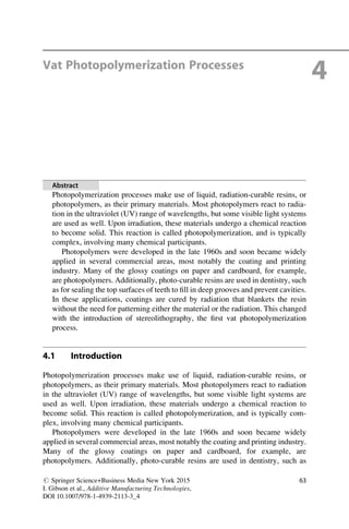
![recoating unnecessary. Approaches that avoid recoating are faster and less
complicated.
In this chapter, we first introduce photopolymer materials, then present the
vector scan SL machines, technologies, and processes. Mask projection approaches
are presented and contrasted with the vector scan approach. Additional
configurations, along with their applications, are presented at the end of the chapter.
Advantages, disadvantages, and uniquenesses of each approach and technology are
highlighted.
4.2 Vat Photopolymerization Materials
Some background of UV photopolymers will be presented in this section that is
common to all configurations of photopolymerization processes. Two subsections
on reaction rates and characterization methods conclude this section. Much of this
material is from the Jacobs book [1] and from a Master’s thesis from the early
2000s [2].
Laser
Optics
Vat
Platform
Scanning
Galvanometers
schematic of vector scan SL
Laser
or Lamp
Optics
DMD
Platform
Vat Vat
Schematic of mask projection approach to
SL.
Two-photon approach
L
a
s
e
r
L
a
s
e
r
a
b
c
Fig. 4.1 Schematic diagrams of three approaches to photopolymerization processes
4.2 Vat Photopolymerization Materials 65](https://image.slidesharecdn.com/1-230308091212-68402451/85/1-Additive-manufacturing-pdf-86-320.jpg)
![4.2.1 UV-Curable Photopolymers
As mentioned, photopolymers were developed in the late 1960s. In addition to the
applications mentioned in Sect. 4.1, they are used as photoresists in the microelec-
tronics industry. This application has had a major impact on the development of
epoxy-based photopolymers. Photoresists are essentially one-layer SL, but with
critical requirements on accuracy and feature resolution.
Various types of radiation may be used to cure commercial photopolymers,
including gamma rays, X-rays, electron beams, UV, and in some cases visible
light, although UV and electron beam are the most prevalent. In AM, many of these
radiation sources have been utilized in research, however only UV and visible light
systems are utilized in commercial systems. In SL systems, for example, UV
radiation is used exclusively although, in principle, other types could be used. In
the SLA-250 from 3D Systems, a helium–cadmium (HeCd) laser is used with a
wavelength of 325 nm. In contrast, the solid-state lasers used in the other SL models
are Nd-YVO4. In mask projection DMD-based systems, UV and visible light
radiation are used.
Thermoplastic polymers that are typically injection molded have a linear or
branched molecular structure that allows them to melt and solidify repeatedly. In
contrast, VP photopolymers are cross-linked and, as a result, do not melt and exhibit
much less creep and stress relaxation. Figure 4.2 shows the three polymer structures
mentioned [3].
The first US patents describing SL resins were published in 1989 and 1990 [4,
5]. These resins were prepared from acrylates, which had high reactivity but
typically produced weak parts due to the inaccuracy caused by shrinkage and
curling. The acrylate-based resins typically could only be cured to 46 % completion
when the image was transferred through the laser [6]. When a fresh coating was put
on the exposed layer, some radiation went through the new coating and initiated
new photochemical reactions in the layer that was already partially cured. This
layer was less susceptible to oxygen inhibition after it had been coated. The
additional cross-linking on this layer caused extra shrinkage, which increased
stresses in the layer, and caused curling that was observed either during or after
the part fabrication process [7].
The first patents that prepared an epoxide composition for SL resins appeared in
1988 [8, 9] (Japanese). The epoxy resins produced more accurate, harder, and
stronger parts than the acrylate resins. While the polymerization of acrylate
compositions leads to 5–20 % shrinkage, the ring-opening polymerization of
epoxy compositions only leads to a shrinkage of 1–2 % [10]. This low level of
shrinkage associated with epoxy chemistry contributes to excellent adhesion and
reduced tendency for flexible substrates to curl during cure. Furthermore, the
polymerization of the epoxy-based resins is not inhibited by atmospheric oxygen.
This enables low-photoinitiator concentrations, giving lower residual odor than
acrylic formulations [11].
However, the epoxy resins have disadvantages of slow photospeed and brittle-
ness of the cured parts. The addition of some acrylate to epoxy resins is required to
66 4 Vat Photopolymerization Processes](https://image.slidesharecdn.com/1-230308091212-68402451/85/1-Additive-manufacturing-pdf-87-320.jpg)
![rapidly build part strength so that they will have enough integrity to be handled
without distortion during fabrication. The acrylates are also useful to reduce the
brittleness of the epoxy parts [7]. Another disadvantage of epoxy resins is their
sensitivity to humidity, which can inhibit polymerization [11].
As a result, most SL resins commercially available today are epoxides with some
acrylate content. It is necessary to have both materials present in the same formula-
tion to combine the advantages of both curing types. The improvement in accuracy
resulting from the use of hybrid resins has given SL a tremendous boost.
4.2.2 Overview of Photopolymer Chemistry
VP photopolymers are composed of several types of ingredients: photoinitiators,
reactive diluents, flexibilizers, stabilizers, and liquid monomers. Broadly speaking,
when UV radiation impinges on VP resin, the photoinitiators undergo a chemical
transformation and become “reactive” with the liquid monomers. A “reactive”
photoinitiator reacts with a monomer molecule to start a polymer chain. Subsequent
reactions occur to build polymer chains and then to cross-link—creation of strong
covalent bonds between polymer chains. Polymerization is the term used to
describe the process of linking small molecules (monomers) into larger molecules
(polymers) composed of many monomer units [1]. Two main types of photopoly-
mer chemistry are commercially evident:
linear
branched
cross-linked
a
b
c
Fig. 4.2 Schematics of
polymer types
4.2 Vat Photopolymerization Materials 67](https://image.slidesharecdn.com/1-230308091212-68402451/85/1-Additive-manufacturing-pdf-88-320.jpg)
![• Free-radical photopolymerization—acrylate
• Cationic photopolymerization—epoxy and vinylether
The molecular structures of these types of photopolymers are shown in Fig. 4.5.
Symbols C and H denote carbon and hydrogen atoms, respectively, while R denotes
a molecular group which typically consists of one or more vinyl groups. A vinyl
group is a molecular structure with a carbon–carbon double bond. It is these vinyl
groups in the R structures that enable photopolymers to become cross-linked.
Free-radical photopolymerization was the first type that was commercially
developed. Such SL resins were acrylates. Acrylates form long polymer chains
once the photoinitiator becomes “reactive,” building the molecule linearly by
adding monomer segments. Cross-linking typically happens after the polymer
chains grow enough so that they become close to one another. Acrylate
photopolymers exhibit high photospeed (react quickly when exposed to UV radia-
tion), but have a number of disadvantages including significant shrinkage and a
tendency to warp and curl. As a result, they are rarely used now without epoxy or
other photopolymer elements.
The most common cationic photopolymers are epoxies, although vinylethers are
also commercially available. Epoxy monomers have rings, as shown in Fig. 4.3.
When reacted, these rings open, resulting in sites for other chemical bonds. Ring-
opening is known to impart minimal volume change on reaction, because the
number and types of chemical bonds are essentially identical before and after
reaction [12]. As a result, epoxy SL resins typically have much smaller shrinkages
and much less tendency to warp and curl. Almost all commercially available SL
resins have significant amounts of epoxies.
Polymerization of VP monomers is an exothermic reaction, with heats of
reaction around 85 kJ/mol for an example acrylate monomer. Despite high heats
of reaction, a catalyst is necessary to initiate the reaction. As described earlier, a
photoinitiator acts as the catalyst.
Schematically, the free radical-initiated polymerization process can be
illustrated as shown in Fig. 4.4 [1]. On average, for every two photons (from the
laser), one radical will be produced. That radical can easily lead to the polymeriza-
tion of over 1,000 monomers, as shown in the intermediate steps of the process,
called propagation. In general, longer polymer molecules are preferred, yielding
higher molecular weights. This indicates a more complete reaction. In Fig. 4.4, the
P–I term indicates a photoinitiator, the I●
symbol is a free radical, and M in a
monomer.
Polymerization terminates from one of three causes, recombination, dispropor-
tionation, or occlusion. Recombination occurs when two polymer chains merge by
joining two radicals. Disproportionation involves essentially the cancelation of one
radical by another, without joining. Occlusion occurs when free radicals become
“trapped” within a solidified polymer, meaning that reaction sites remain available,
but are prevented from reacting with other monomers or polymers by the limited
mobility within the polymer network. These occluded sites will most certainly react
eventually, but not with another polymer chain or monomer. Instead, they will react
68 4 Vat Photopolymerization Processes](https://image.slidesharecdn.com/1-230308091212-68402451/85/1-Additive-manufacturing-pdf-89-320.jpg)
![with oxygen or another reactive species that diffuses into the occluded region. This
may be a cause of aging or other changes in mechanical properties of cured parts,
which should be a topic of future research.
Cationic photopolymerization shares the same broad structure as free-radical
polymerization, where a photoinitiator generates a cation as a result of laser energy,
the cation reacts with a monomer, propagation occurs to generate a polymer, and a
termination process completes the reaction. A typical catalyst for a cationic poly-
merization is a Lewis Acid, such as BF3 [13]. Initially, cationic photopoly-
merization received little attention, but that has changed during the 1990s due to
advances in the microelectronics industry, as well as interest in SL technology. We
H
H
H
H
H
H
H
H
H
C
C
C
C C
C
O
O
O
O
R
R
R
C
Acrylate
Epoxy
Vinylether
a
b
c
Fig. 4.3 Molecular structure
of VP monomers
(initiation)
(free radical formation)
(propagation)
(termination)
P-I
+M
I-M•
I-M•
I-M-M-M-M...-M-I
I-M-M-M-M...-M•
-I•
I•
Fig. 4.4 Free-radical polymerization process
4.2 Vat Photopolymerization Materials 69](https://image.slidesharecdn.com/1-230308091212-68402451/85/1-Additive-manufacturing-pdf-90-320.jpg)
![will not investigate the specifics of cationic reactions here, but will note that the
ring-opening reaction mechanism of epoxy monomers is similar to radical propa-
gation in acrylates.
4.2.3 Resin Formulations and Reaction Mechanisms
Basic raw materials such as polyols, epoxides, (meth) acrylic acids and their esters,
and diisocyanates are used to produce the monomers and oligomers used for
radiation curing. Most of the monomers are multifunctional monomers (MFM) or
polyol polyacrylates which give a cross-linking polymerization. The main chemical
families of oligomers are polyester acrylate (PEA), epoxy acrylates (EA), urethane
acrylates (UA), amino acrylates (used as photoaccelerator in the photoinitiator
system), and cycloaliphatic epoxies [11].
Resin suppliers create ready-to-use formulations by mixing the oligomers and
monomers with a photoinitiator, as well as other materials to affect reaction rates
and part properties. In practice, photosensitizers are often used in combination with
the photoinitiator to shift the absorption towards longer wavelengths. In addition,
supporting materials may be mixed with the initiator to achieve improved solubility
in the formulation. Furthermore, mixtures of different types of photoinitiators may
also be employed for a given application. Thus, photoinitiating systems are, in
practice, often highly elaborate mixtures of various compounds which provide
optimum performance for specific applications [10].
Other additives facilitate the application process and achieve products of good
properties. A reactive diluent, for example, is usually added to adjust the viscosity
of the mixtures to an acceptable level for application [14]; it also participates in the
polymerization reaction.
4.2.3.1 Photoinitiator System
The role of the photoinitiator is to convert the physical energy of the incident light
into chemical energy in the form of reactive intermediates. The photoinitiator must
exhibit a strong absorption at the laser emission wavelength, and undergo a fast
photolysis to generate the initiating species with a great quantum yield [15]. The
reactive intermediates are either radicals capable of adding to vinylic or acrylic
double bonds, thereby initiating radical polymerization, or reactive cationic species
which can initiate polymerization reactions among epoxy molecules [10].
The free-radical polymerization process was outlined in Fig. 4.4, with the
formation of free radicals as the first step. In the typical case in VP, radical
photoinitiator systems include compounds that undergo unimolecular bond cleav-
age upon irradiation. This class includes aromatic carbonyl compounds that are
known to undergo a homolytic C–C bond scission upon UV exposure [16]. The
benzoyl radical is the major initiating species, while the other fragment may, in
some cases, also contribute to the initiation. The most efficient photoinitiators
include benzoin ether derivatives, benzyl ketals, hydroxyalkylphenones, α-amino
70 4 Vat Photopolymerization Processes](https://image.slidesharecdn.com/1-230308091212-68402451/85/1-Additive-manufacturing-pdf-91-320.jpg)
![ketones, and acylphosphine oxides [16, 17]. The Irgacure family of radical
photoinitiators from Ciba Specialty Chemicals is commonly used in VP.
While photoinitiated free-radical polymerizations have been investigated for
more than 60 years, the corresponding photoinduced cationic polymerizations
have received much less attention. The main reason for the slow development in
this area was the lack of suitable photoinitiators capable of efficiently inducing
cationic polymerization [18]. Beginning in 1965, with the earliest work on diazo-
nium salt initiators, this situation has markedly changed. The discovery in the 1970s
of onium salts or organometallic compounds with excellent photoresponse and high
efficiency has initiated the very rapid and promising development of cationic
photopolymerization, and made possible the concurrent radical and cationic reac-
tion in hybrid systems [19]. Excellent reviews have been published in this field [10,
18, 20–23]. The most important cationic photoinitiators are the onium salts, partic-
ularly the triarylsulfonium and diaryliodonium salts. Examples of the cationic
photoinitiator are triaryl sulfonium hexafluorophosphate solutions in propylene
carbonate such as Degacure KI 85 (Degussa), SP-55 (Asahi Denka), Sarcat KI-85
(Sartomer), and 53,113-8 (Aldrich), or mixtures of sulfonium salts such as SR-1010
(Sartomer, currently unavailable), UVI 6976 (B-V), and UVI 6992 (B-VI) (Dow).
Initiation of cationic polymerization takes place from not only the primary
products of the photolysis of triarylsulfonium salts but also from secondary
products of the reaction of those reactive species with solvents, monomers, or
even other photolysis species. Probably the most ubiquitous species present is the
protonic acid derived from the anion of the original salt. Undoubtedly, the largest
portion of the initiating activity in cationic polymerization by photolysis of
triarylsulfonium salts is due to protonic acids [18].
4.2.3.2 Monomer Formulations
The monomer formulations presented here are from a set of patents from the mid- to
late-1990s. Both di-functional and higher functionality monomers are used typi-
cally in VP resins. Poly(meth)acrylates may be tri-, pentafunctional monomeric or
oligomeric aliphatic, cycloaliphatic or aromatic (meth)acrylates, or polyfunctional
urethane (meth)acrylates [24–27]. One specific compound in the Huntsman
SL-7510 resin includes the dipentaerythritol monohydroxy penta(meth)acrylates
[26], such as Dipentaerythritol Pentaacrylate (SR-399, Sartomer).
The cationically curable epoxy resins may have an aliphatic, aromatic, cycloali-
phatic, araliphatic, or heterocyclic structure; they on average possess more than one
epoxide group (oxirane ring) in the molecule and comprise epoxide groups as side
groups, or those groups form part of an alicyclic or heterocyclic ring system.
Examples of epoxy resins of this type are also given by these patents such as
polyglycidyl esters or ethers, poly(N or S-glycidyl) compounds, and epoxide
compounds in which the epoxide groups form part of an alicyclic or heterocyclic
ring system. One specific composition includes at least 50 % by weight of a
cycloaliphatic diepoxide [26] such as bis(2,3-epoxycyclopentyl) ether (formula
A-I), 3,4-epoxycyclohexyl-methyl 3,4-epoxycyclohexanecarboxylate (A-II),
4.2 Vat Photopolymerization Materials 71](https://image.slidesharecdn.com/1-230308091212-68402451/85/1-Additive-manufacturing-pdf-92-320.jpg)
![dicyclopentadiene diepoxide (A-III), and bis-(3,4-epoxycyclohexylmethyl) adipate
(A-IV).
Additional insight into compositions can be gained by investigating the patent
literature further.
4.2.3.3 Interpenetrating Polymer Network Formation
As described earlier, acrylates polymerize radically, while epoxides cationically
polymerize to form their respective polymer networks. In the presence of each other
during the curing process, an interpenetrating polymer network (IPN) is finally
obtained [28, 29]. An IPN can be defined as a combination of two polymers in
network form, at least one of which is synthesized and/or cross-linked in the
immediate presence of the other [30]. It is therefore a special class of polymer
blends in which both polymers generally are in network form [30–32], and which is
originally generated by the concurrent reactions instead of by a simple mechanical
mixing process. In addition, it is a polymer blend rather than a copolymer that is
generated from the hybrid curing [33], which indicates that acrylate and epoxy
monomers undergo independent polymerization instead of copolymerization. How-
ever, in special cases, copolymerization can occur, thus leading to a chemical
bonding of the two networks [34].
It is likely that in typical SL resins, the acrylate and epoxide react independently.
Interestingly, however, these two monomers definitely affect each other physically
during the curing process. The reaction of acrylate will enhance the photospeed and
reduce the energy requirement of the epoxy reaction. Also, the presence of acrylate
monomer may decrease the inhibitory effect of humidity on the epoxy polymeriza-
tion. On the other hand, the epoxy monomer acts as a plasticizer during the early
polymerization of the acrylate monomer where the acrylate forms a network while
the epoxy is still at liquid stage [31]. This plasticizing effect, by increasing
molecular mobility, favors the chain propagation reaction [35]. As a result, the
acrylate polymerizes more extensively in the presence of epoxy than in the neat
acrylate monomer. Furthermore, the reduced sensitivity of acrylate to oxygen in the
hybrid system than in the neat composition may be due to the simultaneous
polymerization of the epoxide which makes the viscosity rise, thus slowing down
the diffusion of atmospheric oxygen into the coating [31].
In addition, it has been shown [31] that the acrylate/epoxide hybrid system
requires a shorter exposure to be cured than either of the two monomers taken
separately. It might be due to the plasticizing effect of epoxy monomer and the
contribution of acrylate monomer to the photospeed of the epoxy polymerization.
The two monomers benefit from each other by a synergistic effect.
It should be noted that if the concentration of the radical photoinitiator was
decreased so that the two polymer networks were generated simultaneously, the
plasticizing effect of the epoxy monomer would become less pronounced. As a
result, it would be more difficult to achieve complete polymerization of the acrylate
monomer and thus require longer exposure time.
Although the acrylate/epoxy hybrid system proceeds via a heterogeneous mech-
anism, the resultant product (IPN) seems to be a uniphase component [36]. The
72 4 Vat Photopolymerization Processes](https://image.slidesharecdn.com/1-230308091212-68402451/85/1-Additive-manufacturing-pdf-93-320.jpg)
![properties appear to be extended rather than compromised [31, 34]. The optimal
properties of IPNs for specific applications can be obtained by selecting two
appropriate components and adjusting their proportions [34]. For example, increas-
ing the acrylate content increases the cure speed but decreases the adhesion
characteristics, while increasing the epoxy content reduces the shrinkage of curing
and improves the adhesion, but decreases the cure speed [36].
4.3 Reaction Rates
As is evident, the photopolymerization reaction in VP resins is very complex. To
date, no one has published an analytical photopolymerization model that describes
reaction results and reaction rates. However, qualitative understanding of reaction
rates is straightforward for simple formulations. Broadly speaking, reaction rates
for photopolymers are controlled by concentrations of photoinitiators [I] and
monomers [M]. The rate of polymerization is the rate of monomer consumption,
which can be shown as [3]:
Rp ¼ d M
½ =dt α M
½ k I
½
ð Þ1=2
ð4:1Þ
where k ¼ constant that is a function of radical generation efficiency, rate of radical
initiation, and rate of radical termination. Hence, the polymerization rate is propor-
tional to the concentration of monomer, but is only proportional to the square root
of initiator concentration.
Using similar reasoning, it can be shown that the average molecular weight of
polymers is the ratio of the rate of propagation and the rate of initiation. This
average weight is called the kinetic average chain length, vo, and is given in (4.2):
vo ¼ Rp=Ri α M
½ = I
½ 1=2
ð4:2Þ
where Ri is the rate of initiation of macromonomers.
Equations (4.1) and (4.2) have important consequences for the VP process. The
higher the rate of polymerization, the faster parts can be built. Since VP resins are
predominantly composed of monomers, the monomer concentration cannot be
changed much. Hence, the only other direct method for controlling the polymeriza-
tion rate and the kinetic average chain length is through the concentration of
initiator. However, (4.1) and (4.2) indicate a trade-off between these characteristics.
Doubling the initiator concentration only increases the polymerization rate by a
factor of 1.4, but reduces the molecular weight of resulting polymers by the same
amount. Strictly speaking, this analysis is more appropriate for acrylate resins, since
epoxies continue to react after laser exposure, so (4.2) does not apply well for
epoxies. However, reaction of epoxies is still limited, so it can be concluded that a
trade-off does exist between polymerization rate and molecular weight for epoxy
resins.
4.3 Reaction Rates 73](https://image.slidesharecdn.com/1-230308091212-68402451/85/1-Additive-manufacturing-pdf-94-320.jpg)
![4.4 Laser Scan Vat Photopolymerization
Laser scan VP creates solid parts by selectively solidifying a liquid photopolymer
resin using an UV laser. As with many other AM processes, the physical parts are
manufactured by fabricating cross-sectional contours, or slices, one on top of
another. These slices are created by tracing 2D contours of a CAD model in a vat
of photopolymer resin with a laser. The part being built rests on a platform that is
dipped into the vat of resin, as shown schematically in Fig. 4.1a. After each slice is
created, the platform is lowered, the surface of the vat is recoated, then the laser
starts to trace the next slice of the CAD model, building the prototype from the
bottom up. A more complete description of the SL process may be found in
[12]. The creation of the part requires a number of key steps: input data, part
preparation, layer preparation, and finally laser scanning of the two-dimensional
cross-sectional slices. The input data consist of an STL file created from a CAD file
or reverse engineering data. Part preparation is the phase at which the operator
specifies support structures, to hold each cross section in place while the part builds,
and provides values for machine parameters. These parameters control how the
prototype is fabricated in the VP machine. Layer preparation is the phase in which
the STL model is divided into a series of slices, as defined by the part preparation
phase, and translated by software algorithms into a machine language. This infor-
mation is then used to drive the SL machine and fabricate the prototype. The laser
scanning of the part is the phase that actually solidifies each slice in the VP
machine.
After building the part, the part must be cleaned, post-cured, and finished.
During the cleaning and finishing phase, the VP machine operator may remove
support structures. During finishing, the operator may spend considerable time
sanding and filing the part to provide the desired surface finishes.
4.5 Photopolymerization Process Modeling
Background on SL materials and energy sources enables us to investigate the curing
process of photopolymers in SL machines. We will begin with an investigation into
the fundamental interactions of laser energy with photopolymer resins. Through the
application of the Beer–Lambert law, the theoretical relationship between resin
characteristics and exposure can be developed, which can be used to specify laser
scan speeds. This understanding can then be applied to investigate mechanical
properties of cured resins. From here, we will briefly investigate the ranges of
size scales and time scales of relevance to the SL process. Much of this section is
adapted from [1].
Nomenclature
Cd ¼ cure depth ¼ depth of resin cure as a result of laser irradiation [mm]
Dp ¼ depth of penetration of laser into a resin until a reduction in irradiance of 1/e is
reached ¼ key resin characteristic [mm]
74 4 Vat Photopolymerization Processes](https://image.slidesharecdn.com/1-230308091212-68402451/85/1-Additive-manufacturing-pdf-95-320.jpg)
![E ¼ exposure, possibly as a function of spatial coordinates [energy/unit area]
[mJ/mm2
]
Ec ¼ critical exposure ¼ exposure at which resin solidification starts to occur
[mJ/mm2
]
Emax ¼ peak exposure of laser shining on the resin surface (center of laser spot)
[mJ/mm2
]
H(x, y, z) ¼ irradiance (radiant power per unit area) at an arbitrary point in the
resin ¼ time derivative of E(x, y, z).[W/mm2
]
PL ¼ output power of laser [W]
Vs ¼ scan speed of laser [mm/s]
W0 ¼ radius of laser beam focused on the resin surface [mm]
4.5.1 Irradiance and Exposure
As a laser beam is scanned across the resin surface, it cures a line of resin to a depth
that depends on many factors. However, it is also important to consider the width of
the cured line as well as its profile. The shape of the cured line depends on resin
characteristics, laser energy characteristics, and the scan speed. We will investigate
the relationships among all of these factors in this subsection.
The first concept of interest here is irradiance, the radiant power of the laser per
unit area, H(x, y, z). As the laser scans a line, the radiant power is distributed over a
finite area (beam spots are not infinitesimal). Figure 4.5 shows a laser scanning a
line along the x-axis at a speed Vs [1]. Consider the z-axis oriented perpendicular to
the resin surface and into the resin, and consider the origin such that the point of
interest, p0
, has an x coordinate of 0. The irradiance at any point x, y, z in the resin is
related to the irradiance at the surface, assuming that the resin absorbs radiation
according to the Beer–Lambert Law. The general form of the irradiance equation
for a Gaussian laser beam is given here as (4.3).
H x; y; z
ð Þ ¼ H x; y; 0
ð Þez=Dp
ð4:3Þ
From this relationship, we can understand the meaning of the penetration depth,
Dp. Setting z ¼ Dp, we get that the irradiance at a depth Dp is about 37 %
(e1
¼ 0.36788) of the irradiance at the resin surface. Thus, Dp is the depth into
the resin at which the irradiance is 37 % of the irradiance at the surface. Further-
more, since we are assuming the Beer–Lambert Law holds, Dp is only a function of
the resin.
Without loss of generality, we will assume that the laser scans along the x-axis
from the origin to point b. Then, the irradiance at coordinate x along the scan line is
given by
4.5 Photopolymerization Process Modeling 75](https://image.slidesharecdn.com/1-230308091212-68402451/85/1-Additive-manufacturing-pdf-96-320.jpg)
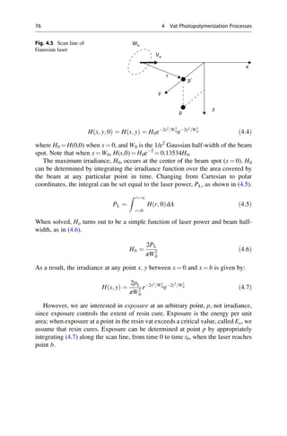
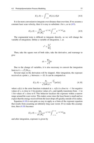
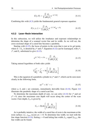
![LW ¼ W0
ffiffiffiffiffiffiffiffiffiffiffiffiffiffiffiffi
2Cd=Dp
q
ð4:17Þ
As a result, two important aspects become clear. First, line width is proportional
to the beam spot size. Second, if a greater cure depth is desired, line width must
increase, all else remaining the same. This becomes very important when
performing line width compensation during process planning.
The final concept to be presented in this subsection is fundamental to commer-
cial SL. It is the working curve, which relates exposure to cure depth, and includes
the two key resin constants, Dp and Ec. At the resin surface and in the center of the
scan line:
E 0; 0
ð Þ Emax ¼
ffiffiffi
2
π
r
PL
W0Vs
ð4:18Þ
which is most of the expression within the logarithm term in (4.16). Substituting
(4.18) into (4.16) yields the working curve equation:
Cd ¼ DP ln
Emax
Ec
ð4:19Þ
In summary, a laser of power PL scans across the resin surface at some speed Vs
solidifying resin to a depth Cd, the cure depth, assuming that the total energy
incident along the scan vector exceeds a critical value called the critical exposure,
Ec. If the laser scans too quickly, no polymerization reaction takes place; i.e.,
exposure E is less than Ec. Ec is assumed to be a characteristic quantity of a
particular resin.
An example working curve is shown in Fig. 4.7, where measured cure depths at a
given exposure are indicated by “*.” The working curve equation, (4.19), has
several major properties [1]:
Z
X Y
Cd
Lw
Fig. 4.6 Cured line showing
parabolic shape, cure depth,
and line width
4.5 Photopolymerization Process Modeling 79](https://image.slidesharecdn.com/1-230308091212-68402451/85/1-Additive-manufacturing-pdf-100-320.jpg)
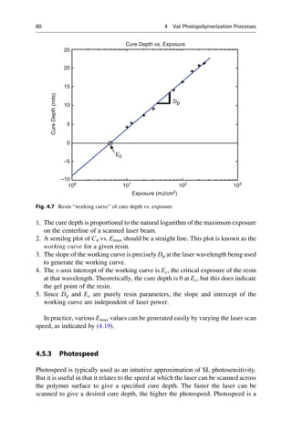
![characteristic of the resin and does not depend upon the specifics of the laser or
optics subsystems. In particular, photospeed is indicated by the resin constants Ec
and Dp, where higher levels of Dp and lower values of Ec indicate higher
photospeed.
To determine scan velocity for a desired cure depth, it is straightforward to solve
(4.16) for Vs. Recall that at the maximum cure depth, the exposure received equals
the cure threshold, Ec. Scan velocity is given by (4.20).
Vs ¼
ffiffiffi
2
π
r
PL
W0Ec
eCd=DP
ð4:20Þ
This discussion can be related back to the working curve. Both Ec and Dp must
be determined experimentally. 3D Systems has developed a procedure called the
WINDOWPANE procedure for finding Ec and Dp values [41]. The cure depth, Cd,
can be measured directly from specimens built on an SL machine that are one layer
thickness in depth. The WINDOWPANE procedure uses a specific part shape, but
the principle is simply to build a part with different amounts of laser exposure in
different places in the part. By measuring the part thickness, Cd, and correlating that
with the exposure values, a “working curve” can easily be plotted. Note that (4.19)
is log-linear. Hence, Cd is plotted linearly vs. the logarithm of exposure to generate
a working curve.
So how is exposure varied? Exposure is varied by simply using different scan
velocities in different regions of the WINDOWPANE part. The different scan
velocities will result in different cure depths. In practice, (4.20) is very useful
since we want to directly control cure depth, and want to determine how fast to
scan the laser to give that cure depth. Of course, for the WINDOWPANE experi-
ment, it is more useful to use (4.16) or (4.19).
4.5.4 Time Scales
It is interesting to investigate the time scales at which SL operates. On the short end
of the time scale, the time it takes for a photon of laser light to traverse a
photopolymer layer is about a picosecond (10–12
s). Photon absorption by the
photoinitiator and the generation of free radicals or cations occur at about the
same time frame. A measure of photopolymer reaction speed is the kinetic reaction
rates, tk, which are typically several microseconds.
The time it takes for the laser to scan past a particular point on the resin surface is
related to the size of the laser beam. We will call this time the characteristic
exposure time, te. Values of te are typically 50–2,000 μs, depending on the scan
speed (500–5,000 mm/s). Laser exposure continues long after the onset of poly-
merization. Continued exposure generates more free radicals or cations and, pre-
sumably, generates these at points deeper in the photopolymer. During and after the
laser beam traverses the point of interest, cross-linking occurs in the photopolymer.
4.5 Photopolymerization Process Modeling 81](https://image.slidesharecdn.com/1-230308091212-68402451/85/1-Additive-manufacturing-pdf-102-320.jpg)
![The onset of measurable shrinkage, ts,o, lags exposure by several orders of
magnitude. This appears to be due to the rate of cross-linking, but for the epoxy-
based resins, may have more complicated characteristics. Time at corresponding
completion of shrinkage is denoted ts,c. For the acrylate-based resins of the early
1990s, times for the onset and completion of shrinkage were typically 0.4–1 and 4–
10 s, respectively. Recall that epoxies can take hours or days to polymerize. Since
shrinkage lags exposure, this is clearly a phenomenon that complicates the VP
process. Shrinkage leads directly to accuracy problems, including deviation from
nominal dimensions, warpage, and curl.
The final time dimension is that of scan time for a layer, denoted td, which
typically spans 10–300 s. The time scales can be summarized as
tt tk te ts,o ts,c td ð4:21Þ
As a result, characteristic times for the VP process span about 14 orders of
magnitude.
4.6 Vector Scan VP Machines
At present (2014), 3D Systems is the predominant manufacturer of laser scanning
VP machines in the world, although several other companies in Japan and else-
where in Asia also market VP machines. Fockele Schwarze in Germany produces
a micro-VP technology, although they only sell design and manufacturing services.
Several Japanese companies produce or produced machines, including Denken
Engineering, CMET (Mitsubishi), Sony, Meiko Corp., Mitsui Zosen, and Teijin
Seiki (license from Dupont). Formlabs is a start-up company, funded in part by a
Kickstarter campaign, markets a small, high-resolution SL machine.
A schematic of a typical VP machine was illustrated in Fig. 4.1a, which shows
the main subsystems, including the laser and optics, the platform and elevator, the
vat and resin-handling subsystem, and the recoater. The machine subsystem hierar-
chy is given in Fig. 4.8. Note that the five main subsystems are: recoating system,
platform system, vat system, laser and optics system, and control system.
Typically, recoating is done using a shallow dip and recoater blade sweeping.
Recoating issues are discussed in [37]. The process can be described as follows:
• After a layer has been cured, the platform dips down by a layer thickness.
• The recoater blade slides over the whole build depositing a new layer of resin
and smoothing the surface of the vat.
A common recoater blade type is the zephyr blade, which is a hollow blade that
is filled with resin. A vacuum system pulls resin into the blade from the vat. As the
blade translates over the vat to perform recoating, resin is deposited in regions
where the previous part cross section was built. When the blade encounters a region
in the vat without resin, the resin falls into this region since its weight is stronger
82 4 Vat Photopolymerization Processes](https://image.slidesharecdn.com/1-230308091212-68402451/85/1-Additive-manufacturing-pdf-103-320.jpg)
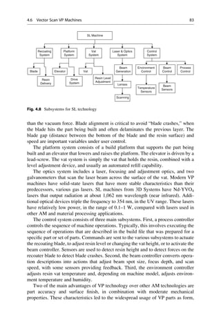
![fit, and, to a lesser extent, functional prototypes. Typical dimensional accuracies for
VP machines are often quoted as a ratio of an error per unit length. For example,
accuracy of an SLA-250 is typically quoted as 0.002 in./in. [38]. Modern VP
machines are somewhat more accurate. Surface finish of SL parts ranges from
submicron Ra for upfacing surfaces to over 100 μm Ra for surfaces at slanted
angles [39].
The current commercial VP product line from 3D Systems consists of two
families of models: the SLA Viper Si2, and the iPro SLA Centers (iPro 9000XL,
iPro 9000, and iPro 8000). Some of these machines are summarized in Table 4.1
[40]. Both the Viper Si2 and the iPro models have dual laser spot size capabilities.
In the Viper Si2, a “high-resolution” mode is available that provides a spot size of
about 80 μm in diameter, useful for building small parts with fine features. In the
iPro machines, in contrast, the machine automatically switches between the “nor-
mal” beam of 0.13 mm diameter for borders and fills and the “wide” beam of
0.76 mm diameter for hatch vectors (filling in large areas). The wide beam enables
much faster builds. The iPro line replaces other machines, including the popular
SLA-3500, SLA-5000, and SLA-7000 machines, as well as the SLA Viper Pro.
Additionally, the SLA-250 was a very popular model that was discontinued in 2001
with the introduction of the Viper Si2 model.
4.7 Scan Patterns
4.7.1 Layer-Based Build Phenomena and Errors
Several phenomena should be noted since they are common to all radiation and
layer-based AM processes. The most obvious phenomenon is discretization, e.g., a
stack of layers causes “stair steps” on slanted or curved surfaces. So, the layer-wise
nature of most AM processes causes edges of layers to be visible. Conventionally,
commercial AM processes build parts in a “material safe” mode, meaning that the
stair steps are on the outside of the CAD part surfaces. Technicians can sand or
finish parts; the material they remove is outside of the desired part geometry. Other
discretization examples are the set of laser scans or the pixels of a DMD. In most
processes, individual laser scans or pixels are not visible on part surfaces, but in
other processes such as material extrusion, the individual filaments can be
noticeable.
As a laser scans a cross section, or a lamp illuminates a layer, the material
solidifies and, as a result, shrinks. When resins photopolymerize, they shrink since
the volume occupied by monomer molecules is larger than that of reacted polymer.
Similarly, after powder melts, it cools and freezes, which reduces the volume of the
material. When the current layer is processed, its shrinkage pulls on the previous
layers, causing stresses to build up in the part. Typically, those stresses remain and
are called residual stresses. Also, those stresses can cause part edges to curl
upwards. Other warpage or part deformations can occur due to these residual
stresses, as well.
84 4 Vat Photopolymerization Processes](https://image.slidesharecdn.com/1-230308091212-68402451/85/1-Additive-manufacturing-pdf-105-320.jpg)
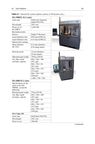
![The last phenomenon to be discussed is that of print-through errors. In
photopolymerization processes, it is necessary to have the current layer cure into
the previous layer. In powder bed fusion processes, the current layer needs to melt
into the previous layer so that one solid part results, instead of a stack of discon-
nected solid layers. The extra energy that extends below the current layer results in
thicker part sections. This extra thickness is called print-through error in SL and
“bonus Z” in laser sintering. Most process planning systems compensate for print-
through by giving users the option of skipping the first few layers of a part, which
works well unless important features are contained within those layers.
These phenomena will be illustrated in this section through an investigation of
scan patterns in SL.
4.7.2 WEAVE
Prior to the development of WEAVE, scan patterns were largely an ad hoc
development. As a result, post-cure curl distortion was the major accuracy problem.
The WEAVE scan pattern became available for use in late 1990 [1].
The development of WEAVE began with the observation that distortion in post-
cured parts was proportional to the percent of uncured resin after removal from the
vat. Another motivating factor was the observation that shrinkage lags exposure and
that this time lag must be considered when planning the pattern of laser scans. The
key idea in WEAVE development was to separate the curing of the majority of a
layer from the adherence of that layer to the previous layer. Additionally, to prevent
Table 4.1 (continued)
Recoating System:
process
Zephyr recoater
Typical 0.1 mm (0.004 in) app.
Minimum 0.05 mm (0.002 in) app.
Optical and scanning
Beam diameter
(@ 1/e2): standard
mode
0.25 0.025 mm
(0.01 0.001 in)
High-resolution 0.075 0.015 mm
(0.003 0.0005 in)
Part drawing speed 5 mm/s (0.2 in/s)
Maximum part weight 9.1 kg (20 lb)
Vat capacity Volume
Maximum build
envelope
250 250 200 mm
XYZ (10 10 10
in)
32.2 L (8.5 U.S. gal)
High-res. build
envelope
125 125 250 mm
(5 5 10 in)
86 4 Vat Photopolymerization Processes](https://image.slidesharecdn.com/1-230308091212-68402451/85/1-Additive-manufacturing-pdf-107-320.jpg)
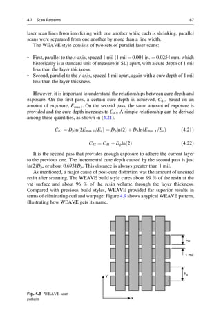
![Even though WEAVE was a tremendous improvement, several flaws were
observed with its usage. Corners were distorted on large flat surfaces, one of
these corners always exhibited larger distortion, and it was always the same corner.
Some microfissures occurred; on a flat plate with a hole, a macrofissure tangent to
the hole would appear.
It was concluded that significant internal stresses developed within parts during
part building, not only post-cure. As a result, improvements to WEAVE were
investigated, leading to the development of STAR-WEAVE.
4.7.3 STAR-WEAVE
STAR-WEAVE was released in October 1991, roughly 1 year after WEAVE
[1]. STAR-WEAVE addressed all of the known deficiencies of WEAVE and
worked very well with the resins available at the time. WEAVE’s deficiencies
were traced to the consequences of two related phenomena: the presence of
shrinkage and the lag of shrinkage relative to exposure. These phenomena led
directly to the presence of large internal stresses in parts. STAR-WEAVE gets its
name from the three main improvements from WEAVE:
1. Staggered hatch
2. Alternating sequence
3. Retracted hatch
Staggered hatch directly addresses the observed microfissures. Consider
Fig. 4.10 which shows a cross-sectional view of the hatch vectors from two layers.
In Fig. 4.10a, the hatch vectors in WEAVE form vertical “walls” that do not directly
touch. In STAR-WEAVE, Fig. 4.10b, the hatch vectors are staggered such that they
directly adhere to the layer below. This resulting overlap from one layer to the next
eliminated microfissures and eliminated stress concentrations in the regions
between vectors.
hs hs
a b
WEAVE STAR-WEAVE
Fig. 4.10 Cross-sectional view of WEAVE and STAR-WEAVE patterns
88 4 Vat Photopolymerization Processes](https://image.slidesharecdn.com/1-230308091212-68402451/85/1-Additive-manufacturing-pdf-109-320.jpg)
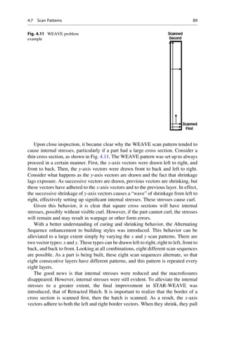
![on the borders, bending them towards one another, causing internal stresses. To
alleviate this, alternating hatch vectors are retracted from the border, as shown in
Fig. 4.12. This retracted hatch is performed for both the x and y vectors.
4.7.4 ACES Scan Pattern
With the development of epoxy-based photopolymers in 1992–1993, new scan
patterns were needed to best adopt to their curing characteristics. ACES (Accurate,
Clear, Epoxy, Solid) was the answer to these needs. ACES is not just a scan pattern,
but is a family of build styles. The operative word in the ACES acronym is
Accurate. ACES was mainly developed to provide yet another leap in part accuracy
by overcoming deficiencies in STAR-WEAVE, most particularly, in percent of
resin cured in the vat. Rather than achieving 96 % solidification, ACES is typically
capable of 98 %, further reducing post-cure shrinkage and the associated internal
stresses, curl, and warpage [12].
Machine operators have a lot of control over the particular scan pattern used,
along with several other process variables. For example, while WEAVE and STAR-
WEAVE utilized 0.001 in. spacings between solidified lines, ACES allows the user
to specify hatch spacing. Table 4.2 shows many of the process variables for the
SLA-250 along with typical ranges of variable settings.
Hatch
Border
0.01 inch
Fig. 4.12 Retracted hatch of
the STAR-WEAVE pattern
Table 4.2 ACES process
variables for the SLA-250
Variable Range
Layer thickness 0.002–0.008 in.
Hatch spacing 0.006–0.012 in.
Hatch overcure (0.003)–(+0.001) in.
Fill overcure 0.006–0.012 in.
Blade gap % 100–200
Sweep period 5–15 s
Z-wait 0–20 s
Pre-dip delay 0–20 s
90 4 Vat Photopolymerization Processes](https://image.slidesharecdn.com/1-230308091212-68402451/85/1-Additive-manufacturing-pdf-111-320.jpg)
![In Table 4.2, the first four variables are called scan variables since they control the
scan pattern, while the remaining variables are recoat variables since they control
how the vat and part are recoated. With this set of variables, the machine operator has
a tremendous amount of control over the process; however, the number of variables
can cause a lot of confusion since it is difficult to predict exactly how the part will
behave as a result of changing a variable’s value. To address this issue, 3D Systems
provides nominal values for many of the variables as a function of layer thickness.
The fundamental premise behind ACES is that of curing more resin in a layer
before bonding that layer to the previous one. This is accomplished by overlapping
hatch vectors, rather than providing 0.001 in. spacing between hatch vectors. As a
result, each point in a layer is exposed to laser radiation from multiple scans. Hence,
it is necessary to consider these multiple scans when determining cure depth for a
layer. ACES also makes use of two passes of scan vectors, one parallel to the x-axis
and one parallel to the y-axis. In the first pass, the resin is cured to a depth 1 mil less
than the desired layer thickness. Then on the second pass, the remaining resin is
cured and the layer is bonded to the previous one.
As might be imagined, more scan vectors are necessary using the ACES scan
pattern, compared with WEAVE and STAR-WEAVE.
The remaining presentation in this section is on the mathematical model of cure
depth as a function of hatch spacing to provide insight into the cure behavior of ACES.
Consider Fig. 4.13 that shows multiple, overlapping scan lines with hatch
spacing hs. Also shown is the cure depth of each line, Cd0, and the cure depth,
160
140
120
100
80
60
40
20
0
–0.05
–0.15
–0.25
–0.35
–0.1
–0.2
–0.3
–0.4
0 0.2
Percent
of
E
max
Cure
Depth
[mm]
0.4 0.6
Y [mm]
0.8 1.0 1.2 1.4
Cd0
EP
hs
Emax
Cd1
Fig. 4.13 Cure depth and exposure for the ACES scan pattern
4.7 Scan Patterns 91](https://image.slidesharecdn.com/1-230308091212-68402451/85/1-Additive-manufacturing-pdf-112-320.jpg)
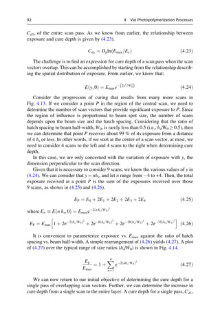
![where areas of the vat surface are illuminated simultaneously to define a part cross
section.
4.8 Vector Scan Micro-Vat Photopolymerization
Several processes were developed exclusively for microfabrication applications
based on photopolymerization principles using both lasers and X-rays as the energy
source. These processes build complex shaped parts that are typically less than
1 mm in size. They are referred to as Microstereolithography (MSL), Integrated
Hardened Stereolithography (IH), LIGA [42], Deep X-ray Lithography (DXRL),
and other names. In this section, we will focus on those processes that utilize UV
radiation to directly process photopolymer materials.
In contrast to convention VP, vector scan technologies for the microscale
typically have moved the vat in x, y, and z directions, rather than scanning the
laser beam. To focus a typical laser to spot sizes less than 20 μm requires the laser’s
focal length to be very short, causing difficulties for scanning the laser. For an
SLA-250 with a 325 nm wavelength HeCd laser, the beam has a diameter of
0.33 mm and a divergence of 1.25 mrad as it exits the laser. It propagates
280 mm then encounters a diverging lens (focal length 25 mm) and a converging
lens (focal length 100 mm) which is 85 mm away. Using simple thin-lens
approximations, the distance from the converging lens to the focal point, where
the laser reaches a spot size of 0.2 mm is 940 mm and its Rayleigh range is 72 mm.
Hence, the focused laser spot is a long distance from the focusing optics and the
Rayleigh range is long enough to enable a wide scanning region and a large
build area.
In contrast, a typical calculation is presented here for a high-resolution micro-SL
system with a laser spot size of 10 μm. A 325 nm wavelength HeCd laser used in SL
is included here to give the reader an idea of the challenge. The beam, as it exits the
laser, has a diameter of 0.33 mm and a divergence of 1.25 mrad. It propagates
280 mm then encounters a diverging lens (focal length 25 mm) and a converging
lens (focal length 36.55 mm). The distance from the converging lens to the focal
point is 54.3 mm and its Rayleigh range is only 0.24 mm. It would be very difficult
to scan this laser beam across a vat without severe spot distortions.
Scanning micro-VP systems have been presented in literature since 1993 with
the introduction of the Integrated Hardening method of Ikuta and Hirowatari
[43]. They used a laser spot focused to a 5-μm diameter and the resin vat is scanned
underneath it to cure a layer. Examples of devices built with this method include
tubes, manifolds, and springs and flexible microactuators [44] and fluid channels on
silicon [45]. Takagi and Nakajima [46] have demonstrated the use of this technol-
ogy for connecting MEMS gears together on a substrate. The artifact fabricated
using micro-VP can be used as a mold for subsequent electroplating followed by
removal of the resin [47]. This method has been able to achieve sub-1 μm minimum
feature size.
94 4 Vat Photopolymerization Processes](https://image.slidesharecdn.com/1-230308091212-68402451/85/1-Additive-manufacturing-pdf-115-320.jpg)
![The following specifications of a typical point-wise microstereolithography
process have been presented in [48]:
• 5-μm spot size of the UV beam
• Positional accuracy is 0.25 μm (in the x–y directions) and 1.0 μm in the z-
direction
• Minimum size of the unit of hardened polymer is 5 μm 5 μm 3 μm (in x, y, z)
• Maximum size of fabrication structure is 10 mm 10 mm 10 mm
The capability of building around inserted components has also been proposed
for components such as ultrafiltration membranes and electrical conductors.
Applications include fluid chips for protein synthesis [49] and bioanalysis
[50]. The bioanalysis system was constructed with integrated valves and pumps
that include a stacked modular design, 13 13 mm2
and 3 mm thick, each of which
has a different fluid function. However, the full extent of integrated processing on
silicon has not yet been demonstrated. The benefits of greater design flexibility and
lower cost of fabrication may be realized in the future.
4.9 Mask Projection VP Technologies and Processes
Technologies to project bitmaps onto a resin surface to cure a layer at a time were
first developed in the early 1990s by researchers who wanted to develop special VP
machines to fabricate microscale parts. Several groups in Japan and Europe pursued
what was called mask projection stereolithography technology at that time. The
main advantage of mask projection methods is speed: since an entire part cross
section can be cured at one time, it can be faster than scanning a laser beam.
Dynamic masks can be realized by LCD screens, by spatial light modulators, or by
DMDs, such as the Digital Light Processing (DLP™) chips manufactured by Texas
Instruments [51].
4.9.1 Mask Projection VP Technology
Mask projection VP (MPVP) systems have been realized by several groups around
the world. Some of the earlier systems utilized LCD displays as their dynamic mask
[52, 53], while another early system used a spatial light modulator [54]. The
remaining systems all used DMDs as their dynamic masks [55–58]. These latest
systems all use UV lamps as their radiation source, while others have used lamps in
the visible range [55] or lasers in the UV. A good overview of micro-VP technol-
ogy, systems, and applications is the book by Varadan et al. [59].
Microscale VP has been commercialized by MicroTEC GmbH, Germany.
Although machines are not for sale, the company offers customer-specific services.
The company has developed machines based on point-wise as well as layer-wise
photopolymerization principles. Their Rapid Micro Product Development (RMPD)
4.9 Mask Projection VP Technologies and Processes 95](https://image.slidesharecdn.com/1-230308091212-68402451/85/1-Additive-manufacturing-pdf-116-320.jpg)
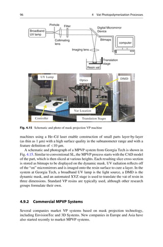
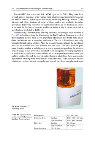
![material feed system. The disadvantage is that small or fine features may be
damaged when the cured layer is separated from the window.
3D Systems introduced their V-Flash machine in 2008. It utilizes MPVP tech-
nology and a novel material handling approach [60]. The V-Flash was intended to
be an inexpensive prototyping machine (under $10,000) that was as easy to use as a
typical home ink-jet printer. Its build envelope was 230 170 200 mm
(9 7 8 in.). During operation, parts were built upside down. For each layer, a
blade coated a layer of resin onto a film that spanned the build chamber. The build
platform slid down until the platform or the in-process part contacted the resin layer
and film. A cartridge provided a supply of unused film for each layer. That layer
was cured by the machine’s “UV Imager,” which consisted of the MPVP technol-
ogy. Some rinsing of the part was required, similar to SL, and support structures
may have to be removed during the post-processing phase of part fabrication.
4.9.3 MPVP Modeling
Most of the research presented on MPVP technology is experimental. As in SL, it is
possible to develop good predictive models of curing for MPVP systems. Broadly
speaking, models of the MPVP process can be described by a model that determines
the irradiation of the vat surface and its propagation into the resin, followed by a
model that determines how the resin reacts to that irradiation. Schematically, the
MPVP model can be given by Fig. 4.17, showing an Irradiance Model and a Cure
Model.
As a given bitmap pattern is displayed, the resin imaged by the “on” mirrors is
irradiated. The exposure received by the resin is simply the product of the irradi-
ance and the time of exposure. The dimensional accuracy of an imaged part cross
Incident beam
characteristics
Imaging system
parameters
Bitmap displayed
on DMD
Lateral
dimensions of
the cured layer
Layer
thickness
Time of
exposure
Irradiance
received by every
point on resin
surface
IRRADIANCE
MODEL
CURE
MODEL
Fig. 4.17 Model of the MPVP process
98 4 Vat Photopolymerization Processes](https://image.slidesharecdn.com/1-230308091212-68402451/85/1-Additive-manufacturing-pdf-119-320.jpg)
![section is a function of the radiation uniformity across the DMD, the collimation of
the beam, and the capability of the optics system in delivering an undistorted image.
If the MPVP machine’s optical system produces a plane wave that is neither
converging nor diverging, then it is easy to project rays from the DMD to the resin
surface. The irradiance model in this case is very straightforward. However, in most
practical cases, it is necessary to model the cone of rays that project from each
micromirror on the DMD to the resin. As a result, a point on the resin may receive
radiation from several micromirrors. Standard ray-tracing methods can be used to
compute the irradiance field that results from a bitmap [61].
After computing the irradiance distribution on the vat surface, the cured shape
can be predicted. The depth of cure can be computed in a manner similar to that
used in Sect. 4.5. Cure depth is computed as the product of the resin’s Dp value and
the exponential of the exposure received divided by the resin’s Ec value, as in
(4.15). The exposure received is simply the product of the irradiance at a point and
the time of exposure, T.
Cd ¼ DPeE=Ec
¼ DPeH T=Ec
ð4:30Þ
In the build direction, overcure and print-through errors are evident, as in SL. In
principle, however, it is easier to correct for these errors than in point-wise SL
systems. A method called the “Compensation Zone” approach was developed to
compensate for this unwanted curing [61]. A tailored volume (Compensation Zone)
is subtracted from underneath the CAD model to compensate for the increase in the
Z dimension that would occur due to print-through. Using this method, more
accurate parts and better surface finish can be achieved.
4.10 Two-Photon Vat Photopolymerization
In the two-photon vat photopolymerization (2p-VP) process, the photoinitiator
requires two photons to strike it before it decomposes to form a free radical that
can initiate polymerization. The effect of this two-photon requirement is to greatly
increase the resolution of photopolymerization processes. This is true since only
near the center of the laser is the irradiance high enough to provide the photon
density necessary to ensure that two photons will strike the same photoinitiator
molecule. Feature sizes of 0.2 μm or smaller have been achieved using 2p-VP.
2p-VP was first invented in the 1970s for the purposes of fabricated three-
dimensional parts [62]. Interestingly, this predates the development of
stereolithography by over 10 years. In this approach, two lasers were used to
irradiate points in a vat of photopolymer. When the focused laser spots intersected,
the photon density was high enough for photopolymerization.
More recently, 2p-VP received research attention in the late 1990s. A schematic
of a typical research setup for this process is shown in Fig. 4.18 [63]. In this system,
they used a high-power Ti:Sapphire laser, with wavelength 790 nm, pulse-width
200 fs, and peak power 50 kW. The objective lens had an NA ¼ 0.85. Similarly to
4.10 Two-Photon Vat Photopolymerization 99](https://image.slidesharecdn.com/1-230308091212-68402451/85/1-Additive-manufacturing-pdf-120-320.jpg)
![other micro-VP approaches, the vat was scanned by a 3D scanning stage, not the
laser beam. Parts were built from the bottom up. The viscosity of the resin was
enough to prevent the micropart being cured from floating away. Complicated parts
have been produced quickly by various research groups. For example, the micro-
bull in Fig. 4.19 was produced in 13 min [64]. The shell of the micro-bull was cured
by 2p-VP, while the interior was cured by flood exposure to UV light.
Typical photopolymer materials can be used in 2p-VP machines [64–66]. The
most commonly used resin was SCR500 from Japan Synthetic Rubber Company,
which was a common SL resin in Japan, where this research started during the
1990s. SCR500 is a mixture of urethane acrylate oligomers/monomers and common
free-radical generating photoinitiators. The absorption spectrum of the resin shows
that it is transparent beyond 550 nm, which is a significant advantage since photons
can penetrate the resin to a great depth (Dp is very large). One implication is that
Computer
Argon ion
laser
Ti:Sapphire
laser
Shutter
CCD camera
Monitor
Objective lens
(N.A. 0.4)
Solidified resin
Lamp
Mirror
3D scanning
stage
Objective lens
(N.A. 0.85)
Photopolymerizable
resin
Fig. 4.18 Schematic of typical two-photon equipment
Fig. 4.19 Bull model fabricated by 2p-VP. The size scale bar is 1 μm
100 4 Vat Photopolymerization Processes](https://image.slidesharecdn.com/1-230308091212-68402451/85/1-Additive-manufacturing-pdf-121-320.jpg)
![parts can be built inside the resin vat, not just at the vat surface, which eliminates
the need for recoating.
Photosensitivity of a 2p-VP resin is measured in terms of the two-photon
absorption cross section (Δ) of the initiator molecule corresponding to the wave-
length used to irradiate it. The larger the value of Δ, the more sensitive is the resin
to two-photon polymerization, possibly enabling lower power lasers.
Acrylate photopolymer systems exhibit low photosensitivity as the initiators
have small two-photon absorption cross sections. Consequently, these initiators
require high-laser power and longer exposure times. Other materials have been
investigated for 2p-VP, specifically using initiators with larger Δ. New types of
photoinitiators tend to be long molecules with certain patterns that make them
particularly good candidates for decomposing into free radicals if two photons
strike it in rapid succession [67]. By tuning the design of the photoinitiators, large
absorption cross sections and low-polymerization threshold energies can be
achieved [68].
4.11 Process Benefits and Drawbacks
Two of the main advantages of vat photopolymerization technology over other AM
technologies are part accuracy and surface finish. These characteristics led to the
widespread usage of vector scan stereolithography parts as form, fit, and, to a lesser
extent, functional prototypes as the rapid prototyping field developed. Typical
dimensional accuracies for SL machines are often quoted as a ratio of an error
per unit length. For example, accuracy of an SLA-250 is typically quoted as
0.002 in./in. Modern SL machines are somewhat more accurate. Surface finish of
SL parts ranges from submicron Ra for upfacing surfaces to over 100 μm Ra for
surfaces at slanted angles.
Another advantage of VP technologies is their flexibility, supporting many
different machine configurations and size scales. Different light sources can be
used, including lasers, lamps, or LEDs, as well as different pattern generators, such
as scanning galvanometers or DMDs. The size range that has been demonstrated
with VP technologies is vast: from the 1.5 m vat in the iPro 9000XL SLA Center to
the 100 nm features possible with 2-photon photopolymerization.
Mask projection VP technologies have an inherent speed advantage over laser
scan SL. By utilizing a mask, an entire part cross section can be projected, rather
than having to sequentially scan the vector pattern for the cross section. There is a
trade-off between resolution and the size of the pattern (and size of the solidified
cross section) due to the mask resolution. For example, typical DMDs have
1,024 780 or 1,280 720 resolution, although newer HDTV DMDs have
resolutions of 1,920 1,080. Nonetheless, for fabricated part resolution of 50 μm
or better, the projected area can be a maximum of 96 54 mm.
A drawback of VP processes is their usage of photopolymers, since the
chemistries are limited to acrylates and epoxies for commercial materials. Although
quite a few other material systems are photopolymerizable, none have emerged as
4.11 Process Benefits and Drawbacks 101](https://image.slidesharecdn.com/1-230308091212-68402451/85/1-Additive-manufacturing-pdf-122-320.jpg)

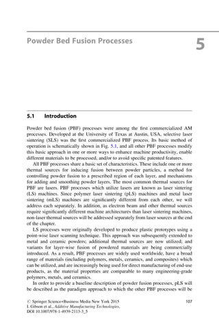
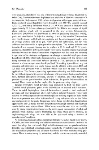
![to produce standard microstructures may be different. As mLS and EBM processes
advance, the types of metal alloys which are commonly utilized will grow and new
alloys specifically tailored for PBF production will be developed.
5.2.3 Ceramics and Ceramic Composites
Ceramic materials are generally described as compounds that consist of metal-
oxides, carbides, and nitrides and their combinations. Several ceramic materials are
available commercially including aluminum oxide and titanium oxide. Commercial
machines were developed by a company called Phenix Systems in France, which
was acquired by 3D Systems in 2013. 3D Systems also says it offers cermets, which
are metal-ceramic composites.
Ceramics and metal-ceramic composites have been demonstrated in research.
Typically, ceramic precipitates form through reactions occurring during the
sintering process. One example is the processing of aluminum in a nitrogen
atmosphere, which forms an aluminum matrix with small regions of AlN
interspersed throughout. This process is called chemically induced sintering and
is described further in the next section.
Biocompatible materials have been developed for specific applications. For
example, calcium hydroxyapatite, a material very similar to human bone, has
been processed using pLS for medical applications.
5.3 Powder Fusion Mechanisms
Since the introduction of LS, each new PBF technology developer has introduced
competing terminology to describe the mechanism by which fusion occurs, with
variants of “sintering” and “melting” being the most popular. However, the use of a
single word to describe the powder fusion mechanism is inherently problematic as
multiple mechanisms are possible. There are four different fusion mechanisms
which are present in PBF processes [1]. These include solid-state sintering, chemi-
cally induced binding, liquid-phase sintering (LPS), and full melting. Most com-
mercial processes utilize primarily LPS and melting. A brief description of each of
these mechanisms and their relevance to AM follows.
5.3.1 Solid-State Sintering
The use of the word sintering to describe powder fusion as a result of thermal
processing predates the advent of AM. Sintering, in its classical sense, indicates the
fusion of powder particles without melting (i.e., in their “solid state”) at elevated
temperatures. This occurs at temperatures between one half of the absolute melting
temperature and the melting temperature. The driving force for solid-state sintering
112 5 Powder Bed Fusion Processes](https://image.slidesharecdn.com/1-230308091212-68402451/85/1-Additive-manufacturing-pdf-133-320.jpg)
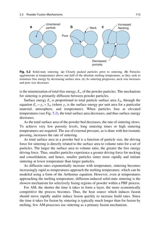
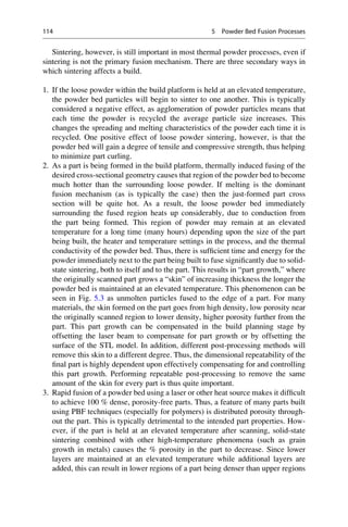
![of a part. This uneven porosity can be controlled, to some extent, by carefully
controlling the part bed temperature, cooling rate and other parameters. EBM, in
particular, often makes use of the positive aspects of elevated-temperature solid-
state sintering and grain growth by purposefully maintaining the metal parts that
are being built at a high enough temperature that diffusion and grain growth
cause the parts being built to reach 100 % density.
5.3.2 Chemically Induced Sintering
Chemically induced sintering involves the use of thermally activated chemical
reactions between two types of powders or between powders and atmospheric
gases to form a by-product which binds the powders together. This fusion mecha-
nism is primarily utilized for ceramic materials. Examples of reactions between
powders and atmospheric gases include: laser processing of SiC in the presence of
oxygen, whereby SiO2 forms and binds together a composite of SiC and SiO2; laser
processing of ZrB2 in the presence of oxygen, whereby ZrO2 forms and binds
together a composite of ZrB2 and ZrO2; and laser processing of Al in the presence
of N2, whereby AlN forms and binds together the Al and AlN particles.
For chemically induced sintering between powders, various research groups
have demonstrated that mixtures of high-temperature structural ceramic and/or
intermetallic precursor materials can be made to react using a laser. In this case,
raw materials which exothermically react to form the desired by-product are
Unmolten
particle fused to
edge
Spherulite from
fully melted
crystallised
particle
Spherulite from
melted
crystallised
region
100 µm
Unmolten
particle core
Fig. 5.3 Typical pLS microstructure for nylon polyamide (Materials Science Engineering.
A. Structural Materials: Properties, Microstructure and Processing by Zarringhalam, H.,
Hopkinson, N., Kamperman, N.F., de Vlieger, J.J. Copyright 2006 by Elsevier Science
Technology Journals. Reproduced with permission of Elsevier Science Technology Journals
in the format Textbook via Copyright Clearance Center) [5]
5.3 Powder Fusion Mechanisms 115](https://image.slidesharecdn.com/1-230308091212-68402451/85/1-Additive-manufacturing-pdf-136-320.jpg)
![pre-mixed and heated using a laser. By adding chemical reaction energy to the laser
energy, high-melting-temperature structures can be created at relatively low laser
energies.
One common characteristic of chemically induced sintering is part porosity. As a
result, post-process infiltration or high-temperature furnace sintering to higher
densities is often needed to achieve properties that are useful for most applications.
This post-process infiltration may involve other reactive elements, forming new
chemical compounds after infiltration. The cost and time associated with post-
processing have limited the adoption of chemically induced sintering in commer-
cial machines.
5.3.3 LPS and Partial Melting
LPS is arguably the most versatile mechanism for PBF. LPS is a term used
extensively in the powder processing industry to refer to the fusion of powder
particles when a portion of constituents within a collection of powder particles
become molten, while other portions remain solid. In LPS, the molten constituents
act as the glue which binds the solid particles together. As a result, high-
temperature particles can be bound together without needing to melt or sinter
those particles directly. LPS is used in traditional powder metallurgy to form, for
instance, cemented carbide cutting tools where Co is used as the lower-melting-
point constituent to glue together particles of WC.
There are many ways in which LPS can be utilized as a fusion mechanism in AM
processes. For purposes of clarity, the classification proposed by Kruth et al. [1] has
formed the basis for the distinctions discussed in the following section and shown in
Fig. 5.4.
5.3.3.1 Distinct Binder and Structural Materials
In many LPS situations, there is a clear distinction between the binding material and
the structural material. The binding and structural material can be combined in
three different ways: as separate particles, as composite particles, or as coated
particles.
Separate Particles
A simple, well-mixed combination of binder and structural powder particles is
sufficient in many cases for LPS. In cases where the structural material has the
dominant properties desired in the final structure, it is advantageous for the binder
material to be smaller in particle size than the structural material. This enables more
efficient packing in the powder bed and less shrinkage and lower porosity after
binding. The dispersion of smaller-particle-size binder particles around structural
particles also helps the binder flow into the gaps between the structural particles
more effectively, thus resulting in better binding of the structural particles. This is
often true when, for instance, LS is used to process steel powder with a polymer
binder (as discussed more fully in Sect. 5.3.5). This is also true when metal-metal
116 5 Powder Bed Fusion Processes](https://image.slidesharecdn.com/1-230308091212-68402451/85/1-Additive-manufacturing-pdf-137-320.jpg)
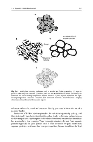
![part properties. Parts held together by polymer binders which require further post-
processing (e.g., to lower or fill the porosity) are termed as “green” parts.
In some cases, the density of the binder and structural material are quite
different. As a result, the binder and structural material may separate during
handling. In addition, some powdered materials are most economically
manufactured at particle sizes that are too small for effective powder dispensing
and leveling (see Sect. 5.5). In either case, it may be beneficial for the structural
and/or binder particles to be bound together into larger particle agglomerates. By
doing so, composite powder particles made up of both binder and structural
material are formed.
Composite Particles
Composite particles contain both the binder and structural material within each
powder particle. Mechanical alloying of binder and structural particles or grinding
of cast, extruded or molded mixtures into a powder results in powder particles that
are made up of binder and structural materials agglomerated together. The benefits
of composite particles are that they typically form higher density green parts and
typically have better surface finish after processing than separate particles [1].
Composite particles can consist of mixtures of polymer binders with higher
melting point polymer, metal, or ceramic structural materials; or metal binders with
higher melting point metal or ceramic structural materials. In all cases, the binder
and structural portions of each particle, if viewed under a microscope, are distinct
from each other and clearly discernable. The most common commercially available
composite particle used in PBF processes is glass-filled nylon. In this case, the
structural material (glass beads) is used to enhance the properties of the binding
material (nylon) rather than the typical use of LPS where the binder is simply a
necessary glue to help hold the structural material together in a useful
geometric form.
Coated Particles
In some cases, a composite formed by coating structural particles with a binder
material is more effective than random agglomerations of binder and structural
materials. These coated particles can have several advantages; including better
absorption of laser energy, more effective binding of the structural particles, and
better flow properties.
When composite particles or separate particles are processed, the random distri-
bution of the constituents means that impinging heat energy, such as laser radiation,
will be absorbed by whichever constituent has the highest absorptivity and/or most
direct “line-of-sight” to the impinging energy. If the structural materials have a
higher absorptivity, a greater amount of energy will be absorbed in the structural
particles. If the rate of heating of the structural particles significantly exceeds the
rate of conduction to the binder particles, the higher-melting-temperature structural
materials may melt prior to the lower-melting-temperature binder materials. As a
result, the anticipated microstructure of the processed material will differ signifi-
cantly from one where the binder had melted and the structural material had
118 5 Powder Bed Fusion Processes](https://image.slidesharecdn.com/1-230308091212-68402451/85/1-Additive-manufacturing-pdf-139-320.jpg)
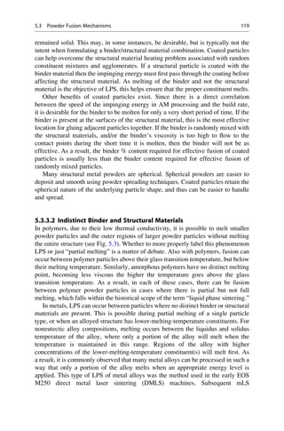
![commercialized processes are all designed to fully melt the metal alloys they
process.
5.3.4 Full Melting
Full melting is the mechanism most commonly associated with PBF processing of
engineering metal alloys and semi-crystalline polymers. In these materials, the
entire region of material subjected to impinging heat energy is melted to a depth
exceeding the layer thickness. Thermal energy of subsequent scans of a laser or
electron beam (next to or above the just-scanned area) is typically sufficient to
re-melt a portion of the previously solidified solid structure; and thus, this type of
full melting is very effective at creating well-bonded, high-density structures from
engineering metals and polymers.
The most common material used in PBF processing is nylon polyamide. As a
semi-crystalline material, it has a distinct melting point. In order to produce parts
with the highest possible strength, these materials should be fully melted during
processing. However, elevated temperatures associated with full melting result in
part growth and thus, for practical purposes, many accuracy versus strength opti-
mization studies result in parameters which are at the threshold between full
melting and LPS, as can be seen from Fig. 5.3.
For metal PBF processes, the engineering alloys that are utilized in these
machines (Ti, Stainless Steel, CoCr, etc.) are typically fully melted. The rapid
melting and solidification of these metal alloys results in unique properties that are
distinct from, and can sometime be more desirable than, cast or wrought parts made
from identical alloys.
Figure 5.5 summarizes the various binding mechanisms which are utilized in
PBF processes. Regardless of whether a technology is known as “Selective Laser
Sintering,” “Selective Laser Melting,” “Direct Metal Laser Sintering,” “Laser
Cusing,” “Electron Beam Melting,” or some other name, it is possible for any of
Primary Binding Mechanisms in Powder Bed Fusion Processes
1. Solid State
Sintering
2. Chemically Induced
Binding
3.1 Distinct binder and
structural materials
3.1.1 Separate particles
3.1.2 Composite particles
3.1.3 Coated particles
3.2 Indistinct binder and
structural materials
3. Liquid Phase Sintering
(Partial Melting)
4. Full Melting
Fig. 5.5 Primary binding mechanisms in powder bed fusion processes (adapted from [1])
120 5 Powder Bed Fusion Processes](https://image.slidesharecdn.com/1-230308091212-68402451/85/1-Additive-manufacturing-pdf-141-320.jpg)
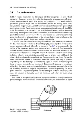
![5.4.2 Applied Energy Correlations and Scan Patterns
Many common physics, thermodynamics, and heat transfer models are relevant to
PBF techniques. In particular, solutions for stationary and moving point-heat-
sources in an infinite media and homogenization equations (to estimate, for
instance, powder bed thermo-physical properties based upon powder morphology,
packing density, etc.) are commonly utilized. The solidification modeling discussed
in the directed energy deposition (DED) chapter (Chap. 10) can also be applied to
PBF processes. For the purposes of this chapter, a highly simplified model which
estimates the energy-input characteristics of PBF processes is introduced and
discussed with respect to process optimization for PBF processes.
Melt pool formation and characteristics are fundamentally determined by the
total amount of applied energy which is absorbed by the powder bed as the laser
beam passes. Both the melt pool size and melt pool depth are a function of absorbed
energy density. A simplified energy density equation has been used by numerous
investigators as a simple method for correlating input process parameters to the
density and strength of produced parts [2]. In their simplified model, applied energy
density EA (also known as the Andrews number) can be found using (5.1):
EA ¼ P= U SP
ð Þ ð5:1Þ
where P is laser power, U is scan velocity, and SP is the scan spacing between
parallel scan lines. In this simplified model, applied energy increases with increas-
ing laser power and decreases with increasing velocity and scan spacing. For pLS,
typical scan spacing values are ~100 μm, whereas typical laser spot sizes are
~300 μm. Thus, typically every point is scanned by multiple passes of the
laser beam.
Although (5.1) does not include powder absorptivity, heat of fusion, laser spot
size, bed temperature, or other important characteristics, it provides the simplest
analytical approach for optimizing machine performance for a material. For a given
material, laser spot size and machine configuration, a series of experiments can be
run to determine the minimum applied energy necessary to achieve adequate
material fusion for the desired material properties. Subsequently, build speed can
be maximized by utilizing the fastest combination of laser power, scan rate, and
scan spacing for a particular machine architecture based upon (5.1).
Optimization of build speed using applied energy is reasonably effective for PBF
of polymer materials. However, when a molten pool of metal is present on a powder
bed, a phenomenon called balling often occurs. When surface tension forces
overcome a combination of dynamic fluid, gravitational and adhesion forces, the
molten metal will form a ball. The surface energy driving force for metal powders
to limit their surface area to volume ratio (which is minimized as a sphere) is much
greater than the driving force for polymers, and thus this phenomenon is unimpor-
tant for polymers but critically important for metals. An example of balling
tendency at various power, P, and scan speed, U, combinations is shown in
5.4 Process Parameters and Modeling 125](https://image.slidesharecdn.com/1-230308091212-68402451/85/1-Additive-manufacturing-pdf-146-320.jpg)
![Fig. 5.8 [3]. This figure illustrates five typical types of tracks which are formed at
various process parameter combinations.
A process map showing regions of power and scan speed combinations which
result in each of these track types is shown in Fig. 5.9. As described by Childs
et al. tracks of type A were continuous and flat topped or slightly concave. At
slightly higher speeds, type B tracks became rounded and sank into the bed. As the
speed increased, type C tracks became occasionally broken, although not with the
regularity of type D tracks at higher speeds, whose regularly and frequently broken
tracks are perfect examples of the balling effect. At even higher speeds, fragile
tracks were formed (type E) where the maximum temperatures exceed the solidus
temperature but do not reach the liquidus temperature (i.e., partially melted or
a b c d e
P(W)
U(mm/s)
110
0.5
Track type
Direction
of
scan
110
2
110
15
110
25
77
40
Fig. 5.8 Five examples of
test tracks made in 150/
+75 μm M2 steel powder in
an argon atmosphere with a
CO2 laser beam of 1.1 mm
spot size, at similar
magnifications (#
Professional Engineering
Publishing, reproduced from
T H C Childs, C Hauser, and
M Badrossamay, Proceedings
of the Institution of
Mechanical Engineers, Part
B: Journal of Engineering
Manufacture 219 (4), 2005)
Fig. 5.9 Process map for
track types shown in Fig. 5.8
(# Professional Engineering
Publishing, reproduced from
T H C Childs, C Hauser, and
M Badrossamay, Proceedings
of the Institution of
Mechanical Engineers, Part
B: Journal of Engineering
Manufacture 219 (4), 2005)
126 5 Powder Bed Fusion Processes](https://image.slidesharecdn.com/1-230308091212-68402451/85/1-Additive-manufacturing-pdf-147-320.jpg)
![layers created by this counter-rotating roller are small, and thus the previously
processed layers are relatively undisturbed.
Another commonly utilized solution for powder spreading is a doctor blade. A
doctor blade is simply a thin piece of metal that is used to scrape material across the
surface of a powder bed. When a doctor blade is used, the powder is not fluidized.
Thus, the shear forces applied to the previously deposited layer are greater than for
a counter-rotating roller. This increased shear can be reduced if the doctor blade is
ultrasonically vibrated, thus partly fluidizing the powder being pushed.
An alternative approach to using a feed cartridge as a powder reservoir is to use a
hopper feeding system. A hopper system delivers powder to the powder bed from
above rather than beneath. The powder reservoir is typically separate from the build
area, and a feeding system is used to fill the hopper. The hopper is then used to
deposit powder in front of a roller or doctor blade, or a doctor blade or roller can be
integrated with a hopper system for combined feeding and spreading. For both
feeding and spreading, ultrasonic vibration can be utilized with any of these
approaches to help fluidize the powders. Various types of powder feeding systems
are illustrated in Fig. 5.10.
In the case of multimaterial powder bed processing, the only effective method is
to use multiple hoppers with separate materials. In a multi-hopper system, the
material type can be changed layer-by-layer. Although this has been demonstrated
in a research environment, and by some companies for very small parts; to date, all
PBF technologies offered for sale commercially utilize a single-material powder
feeding system.
5.5.3 Powder Recycling
As mentioned in Sect. 5.3.1, elevated temperature sintering of the powder
surrounding a part being built can cause the powder bed to fuse. In addition,
elevated temperatures, particularly in the presence of reacting atmospheric gases,
will also change the chemical nature of the powder particles. Similarly, holding
Hopper
Feed
Direction
Doctor blade
Newly
deposited
layer
Feed
Direction
Hopper
Powder
Roller
Newly
deposited
layer
Platform Platform
a b
Fig. 5.10 Examples of hopper-based powder delivery systems [6]
5.5 Powder Handling 129](https://image.slidesharecdn.com/1-230308091212-68402451/85/1-Additive-manufacturing-pdf-150-320.jpg)
![polymer materials at elevated temperatures can change the molecular weight of the
polymer. These combined effects mean that the properties of many different types
of powders (particularly polymers) used in PBF processes change their properties
when they are recycled and reused. For some materials these changes are small, and
thus are considered highly recyclable or infinitely recyclable. In other materials
these changes are dramatic, and thus a highly controlled recycling methodology
must be used to maintain consistent part properties between builds.
For the most popular PBF polymer material, nylon polyamide, both the effective
particle size and molecular weight change during processing. As a result, a number
of recycling methodologies have been developed to seek to maintain consistent
build properties. The simplest approach to this recycling problem is to mix a
specific ratio of unused powder with used powders. An example of a fraction-
based mixture might be 1/3 unused powder, 1/3 overflow/feed powder, and 1/3
build platform powder. Overflow/feed and loose part-bed powder are handled
separately, as they experience different temperature profiles during the build. The
recaptured overflow/feed materials are only slightly modified from the original
material as they have been subjected to lower temperatures only in the feed and
overflow cartridges; whereas, loose part-bed powder from the build platform has
been maintained at an elevated temperature, sometimes for many hours.
Part-bed powder is typically processed using a particle sorting method, most
commonly either a vibratory screen-based sifting device or an air classifier, before
mixing with other powders. Air classifiers can be better than simple sifting, as they
mix the powders together more effectively and help break up agglomerates, thus
enabling a larger fraction of material to be recycled. However, air classifiers are
more complex and expensive than sifting systems. Regardless of the particle sorting
method used, it is critical that the material be well-mixed during recycling; other-
wise, parts built from recycled powder will have different properties in different
locations.
Although easy to implement, a simple fraction-based recycling approach will
always result in some amount of mixing inconsistencies. This is due to the fact that
different builds have different part layout characteristics and thus the loose part-bed
powder being recycled from one build has a different thermal history than loose
part-bed powder being recycled from a different build.
In order to overcome some of the build-to-build inconsistencies inherent in
fraction-based mixing, a recycling methodology based upon a powder’s melt flow
index (MFI) has been developed [4]. MFI is a measure of molten thermoplastic
material flow through an extrusion apparatus under prescribed conditions. ASTM
and ISO standards, for instance, can be followed to ensure repeatability. When
using an MFI-based recycling methodology, a user determines a target MFI, based
upon their experience. Used powders (part-bed and overflow/feed materials) are
mixed and tested. Unused powder is also tested. The MFI for both is determined,
and a well-blended mixture of unused and used powder is created and subsequently
tested to achieve the target MFI. This may have to be done iteratively if the target
MFI is not reached by the first mixture of unused to used powder. Using this
methodology, the closer the target MFI is to the new powder MFI, the higher the
130 5 Powder Bed Fusion Processes](https://image.slidesharecdn.com/1-230308091212-68402451/85/1-Additive-manufacturing-pdf-151-320.jpg)
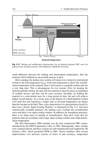
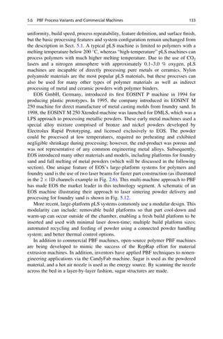
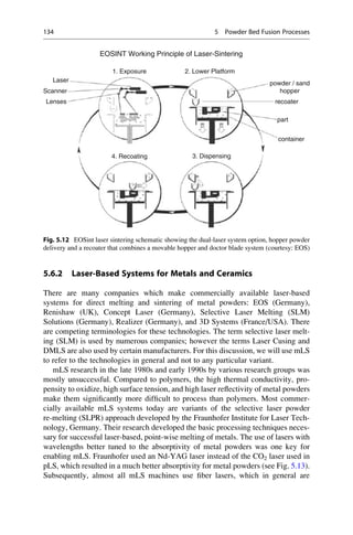
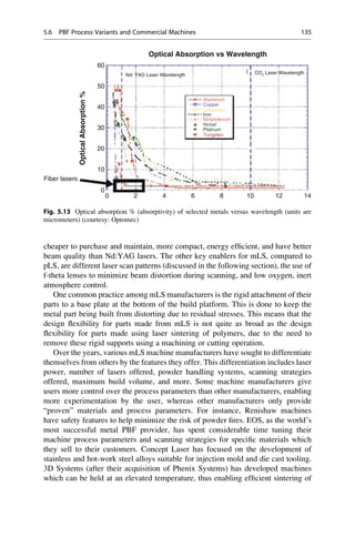
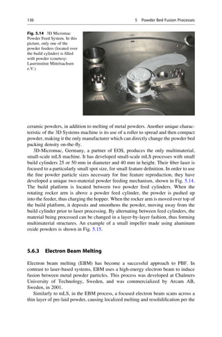
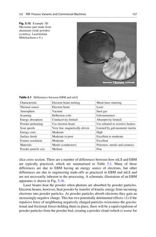
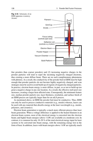
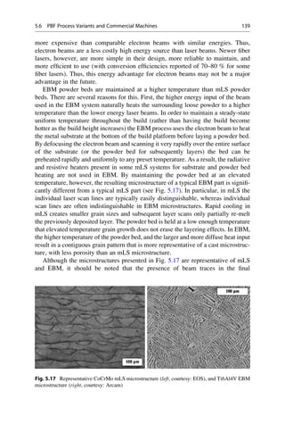
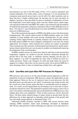

![vertically mounted on a plotting system rather than remaining in a fixed horizontal
position.
An alternative approach is to use a chemical change to cause solidification. In
such cases, a curing agent, residual solvent, reaction with air, or simply drying of a
“wet” material permits bonding to occur. Parts may therefore cure or dry out to
become fully stable. This approach is can be utilized with paste materials. Addi-
tionally, it may be more applicable to biochemical applications where materials
must have biocompatibility with living cells and so choice of material is very
restricted. However, industrial applications may also exist, perhaps using reaction
injection molding-related processes rather than relying entirely on thermal effects.
This chapter will start off by describing the basic principles of extrusion-based
additive manufacturing. Following this will be a description of the most widely
used extrusion-based technology, developed and commercialized by the Stratasys
company. Bioplotting equipment for tissue engineering and scaffold applications
commonly use extrusion technology and a discussion on how this differs from the
Stratasys approach will ensue. Finally, there have been a number of interesting
research projects employing, adapting, and developing this technology, and this
will be covered at the end of the chapter.
6.2 Basic Principles
There are a number of key features that are common to any extrusion-based system:
– Loading of material
– Liquification of the material
– Application of pressure to move the material through the nozzle
– Extrusion
– Plotting according to a predefined path and in a controlled manner
– Bonding of the material to itself or secondary build materials to form a coherent
solid structure
– Inclusion of support structures to enable complex geometrical features
These will be considered in separate sections to fully understand the intricacies
of extrusion-based AM.
A mathematical or physics-based understanding of extrusion processes can
quickly become complex, since it can involve many nonlinear terms. The basic
science involves extrusion of highly viscous materials through a nozzle. It is
reasonable to assume that the material flows as a Newtonian fluid in most cases
[1]. Most of the discussion in these sections will assume the extrusion is of molten
material and may therefore include temperature terms. For solidification, these
temperature terms are generally expressed relative to time; and so temperature
could be replaced by other time-dependent factors to describe curing or drying
processes.
148 6 Extrusion-Based Systems](https://image.slidesharecdn.com/1-230308091212-68402451/85/1-Additive-manufacturing-pdf-168-320.jpg)
![large relative to the nozzle diameter to faithfully reproduce them with satisfactory
strength. Extrusion-based processes are therefore more suitable for larger parts that
have features and wall thicknesses that are at least twice the nominal diameter of the
extrusion nozzle used.
Material flow through the nozzle is controlled by the pressure drop between the
chamber and the surrounding atmosphere. However, the extrusion process used for
AM may not be the same as conventional extrusion. For example, the pressure
developed to push the molten material through the nozzle is typically not generated
by a screw mechanism. However, to understand the process it may be useful to
study a traditional screw-fed extrusion process as described, for example, by
Stevens and Covas [2]. Mass flow through a nozzle is related to pressure drop,
nozzle geometry, and material viscosity. The viscosity is of course primarily a
function of temperature. Since no special dies or material mixing is required for this
type of application, it can be said to behave in a similar manner to a single
Archimedean screw extruder as shown in Fig. 6.2.
Using simple screw geometry, molten material will gradually move along the
screw channel towards the end of the screw where the nozzle is. The velocity W of
material flow along the channel will be
W ¼ πDN cos ϕ ð6:1Þ
where D is the screw diameter, N is the screw speed, and ϕ is the screw angle. The
velocity of the material U towards the nozzle is therefore
Fig. 6.1 Schematic of
extrusion-based systems
150 6 Extrusion-Based Systems](https://image.slidesharecdn.com/1-230308091212-68402451/85/1-Additive-manufacturing-pdf-170-320.jpg)
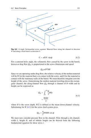
![This provides us with an expression that describes the flow of material back up the
rectangular channel as well as down the screw feed, therefore modeling the drag
flow generated by the screw and the back flow generated by the pressure differential
of the chamber and the output nozzle. A similar pressure flow expression can be
formulated for a circular nozzle to model the extrusion process itself. It is assumed
that only melt flow exists and that there is a stable and constant temperature within
the melt chamber. Both of these are reasonable assumptions.
If a pinch roller feed system is used like in Fig. 6.1, which is in fact the most
common approach, one can consider the forces generated by the rollers as the
mechanism for generating the extrusion pressure. If the force generated by the
rollers exceeds the exit pressure then buckling will occur in the filament feedstock,
assuming there is no slippage between the material and the rollers. An excellent
model analysis of the pinch roller feed system can be found in Turner et al. [3]. This
analysis indicates that the feed forces are related to elastic modulus and that the
more brittle the material, the more difficult it is to feed it through the nozzle. This
would mean that composite materials that use ceramic fillers for example will
require very precise control of feed rates. The increased modulus would lead to
higher pressure and thus a higher force generated by the pinch rollers. The greater
therefore is the chance of slippage or a mismatch between input and output that
would result in non-flow or buckling at the liquifier entry point.
6.2.4 Solidification
Once the material is extruded, it should ideally remain the same shape and size.
Gravity and surface tension, however, may cause the material to change shape,
while size may vary according to cooling and drying effects. If the material is
extruded in the form of a gel, the material may shrink upon drying, as well as
possibly becoming porous. If the material is extruded in a molten state, it may also
shrink when cooling. The cooling is also very likely to be nonlinear. If this
nonlinear effect is significant, then it is possible the resulting part will distort
upon cooling. This can be minimized by ensuring the temperature differential
between the chamber and the surrounding atmosphere is kept to a minimum (i.e.,
use of a controlled environmental chamber when building the part) and also by
ensuring the cooling process is controlled with a gradual and slow profile.
It is reasonable to assume that an extrusion-based AM system will extrude from
a large chamber to a small nozzle through the use of a conical interface. As
mentioned before, the melt is generally expected to adhere to the walls of the
liquefier and nozzle with zero velocity at these boundaries, subjecting the material
to shear deformation during flow. The shear rate _
γ can be defined as [1]
_
γ ¼
dv
dr
ð6:10Þ
and the shear stress as
6.2 Basic Principles 153](https://image.slidesharecdn.com/1-230308091212-68402451/85/1-Additive-manufacturing-pdf-173-320.jpg)
![6.2.6 Bonding
For heat-based systems there must be sufficient residual heat energy to activate the
surfaces of the adjacent regions, causing bonding. Alternatively, gel or paste-based
systems must contain residual solvent or wetting agent in the extruded filament to
ensure the new material will bond to the adjacent regions that have already been
deposited. In both cases, we visualize the process in terms of energy supplied to the
material by the extrusion head.
If there is insufficient energy, the regions may adhere, but there would be a
distinct boundary between new and previously deposited material. This can repre-
sent a fracture surface where the materials can be easily separated. Too much
energy may cause the previously deposited material to flow, which in turn may
result in a poorly defined part.
Once the material has been extruded, it must solidify and bond with adjacent
material. Yardimci defined a set of governing equations that describe the thermal
processes at work in a simple extruded road, laid down in a continuous, open-ended
fashion along a direction x, based on various material properties [5].
ρ
∂q
∂t
¼ k
∂
2
T
∂x2
Sc S1 ð6:12Þ
where ρ is the material density, q is the specific enthalpy, and k the effective thermal
conductivity. T is the cross-sectional average road temperature. The term Sc is a
sink term that describes convective losses.
Fig. 6.3 A typical fill pattern using an extrusion-based system, created in three stages (adapted
from [4])
6.2 Basic Principles 155](https://image.slidesharecdn.com/1-230308091212-68402451/85/1-Additive-manufacturing-pdf-175-320.jpg)
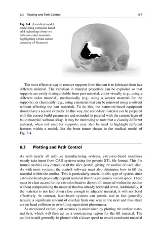
![flow. The outline is determined by extracting intersections between a plane
(representing the current cross section of the build) and the triangles in the STL
file. These intersections are then ordered so that they form a complete, continuous
curve for each outline (there may be any number of these curves, either separate or
nested inside of each other, depending upon the geometry of that cross section). The
only remaining thing for the software to do at this stage is to determine the start
location for each outline. Since the extrusion nozzle is a finite diameter, this start
location is defined by the center of the nozzle. The stop location will be the final
point on this trajectory, located approximately one nozzle diameter from the start
location. Since it is better to have a slight overlap than a gap and because it is very
difficult to precisely control flow, there is likely to be a slight overfill and thus
swelling in this start/stop region. If all the start/stop regions are stacked on top of
each other, then there will be a “seam” running down the part. In most cases, it is
best to have the start/stop regions randomly or evenly distributed around the part so
that this seam is not obvious. However, a counter to this may be that a seam is
inevitable and having it in an obvious region will make it more straightforward for
removing during the post-processing stage.
Determining the fill pattern for the interior of the outlines is a much more
difficult task for the control software. The first consideration is that there must be
an offset inside the outline and that the extrusion nozzle must be placed inside this
outline with minimal overlap. The software must then establish a start location for
the fill and determine the trajectory according to a predefined fill pattern. This fill
pattern is similar to those used in CNC planar pocket milling where a set amount of
material must be removed with a cylindrical cutter [5]. As with CNC milling, there
is no unique solution to achieving the filling pattern. Furthermore, the fill pattern
may not be a continuous, unbroken trajectory for a particular shape. It is preferable
to have as few individual paths as possible but for complex patterns an optimum
value may be difficult to establish. As can be seen with even the relatively simple
cross section in Fig. 6.3, start and stop locations can be difficult to determine and are
somewhat arbitrary. Even with a simpler geometry, like a circle that could be filled
continuously using a spiral fill pattern, it is possible to fill from the outside-in or
from the inside-out.
Spiral patterns in CNC are quite common, mainly because it is not quite so
important as to how the material is removed from a pocket. However, they are less
common as fill patterns for extrusion-based additive manufacturing, primarily for
the following reason. Consider the example of building a simple solid cylinder. If a
spiral pattern were used, every path on every layer would be directly above each
other. This could severely compromise part strength and a weave pattern would be
much more preferable. As with composite material weave patterning using material
like carbon fiber, for example, it is better to cross the weave over each other at an
angle so that there are no weakened regions due to the directionality in the fibers.
Placing extrusion paths over each other in a crossing pattern can help to distribute
the strength in each part more evenly.
Every additional weave pattern within a specific layer is going to cause a
discontinuity that may result in a weakness within the corresponding part. For
158 6 Extrusion-Based Systems](https://image.slidesharecdn.com/1-230308091212-68402451/85/1-Additive-manufacturing-pdf-178-320.jpg)
![complex geometries, it is important to minimize the number of fill patterns used in a
single layer. As mentioned earlier, and illustrated in Fig. 6.3, it is not possible to
ensure that only one continuous fill pattern will successfully fill a single layer. Most
outlines can be filled with a theoretically infinite number of fill pattern solutions. It
is therefore unlikely that a software solution will provide the best or optimum
solution in every case, but an efficient solution methodology should be designed to
prevent too many separate patterns from being used in a single layer.
Parts are weakened as a result of gaps between extruded roads. Since weave
patterns achieve the best mechanical properties if they are extruded in a continuous
path, there are many changes in direction. The curvature in the path for these
changes in direction can result in gaps within the part as illustrated in Fig. 6.5.
This figure illustrates two different ways to define the toolpath, one that will ensure
no additional material will be applied to ensure no part swelling and good part
accuracy. The second approach defines an overlap that will cause the material to
flow into the void regions, but which may also cause the part to swell. However, in
both cases gaps are constrained within the outline material laid down at the
perimeter. Additionally, by changing the flow rate at these directional change
regions, less or more material can be extruded into these regions to compensate
for gaps and swelling. This means that the material flow from the extrusion head
should not be directly proportional to the instantaneous velocity of the head when
the velocity is low, but rather should be increased or decreased slightly, depending
on the toolpath strategy used. Furthermore, if the velocity is zero but the machine is
known to be executing a directional change in a weave path, a small amount of flow
should ideally be maintained. This will cause the affected region to swell slightly
and thus help fill gaps. Obviously, care should be taken to ensure that excess
material is not extruded to the extent that part geometry is compromised [6].
It can be seen that precise control of extrusion is a complex trade-off, dependent
on a significant number of parameters, including:
Actual tool path
Key
Deposited material boundary
Fig. 6.5 Extrusion of materials to maximize precision (left) or material strength (right) by
controlling voids
6.3 Plotting and Path Control 159](https://image.slidesharecdn.com/1-230308091212-68402451/85/1-Additive-manufacturing-pdf-179-320.jpg)
![– Input pressure: This variable is changed regularly during a build, as it is tightly
coupled with other input control parameters. Changing the input pressure
(or force applied to the material) results in a corresponding output flow rate
change. A number of other parameters, however, also affect the flow to a lesser
degree.
– Temperature: Maintaining a constant temperature within the melt inside the
chamber would be the ideal situation. However, small fluctuations are inevitable
and will cause changes in the flow characteristics. Temperature sensing should
be carried out somewhere within the chamber and therefore a loosely coupled
parameter can be included in the control model for the input feed pressure to
compensate for thermal variations. As the heat builds up, the pressure should
drop slightly to maintain the same flow rate.
– Nozzle diameter: This is constant for a particular build, but many extrusion-
based systems do allow for interchangeable nozzles that can be used to offset
speed against precision.
– Material characteristics: Ideally, control models should include information
regarding the materials used. This would include viscosity information that
would help in understanding the material flow through the nozzle. Since viscous
flow, creep, etc. are very difficult to predict, accurately starting and stopping
flow can be difficult.
– Gravity and other factors: If no pressure is applied to the chamber, it is possible
that material will still flow due to the mass of the molten material within the
chamber causing a pressure head. This may also be exacerbated by gaseous
pressure buildup inside the chamber if it is sealed. Surface tension of the melt
and drag forces at the internal surfaces of the nozzle may retard this effect.
– Temperature build up within the part: All parts will start to cool down as soon as
the material has been extruded. However, different geometries will cool at
different rates. Large, massive structures will hold their heat for longer times
than smaller, thinner parts, due to the variation in surface to volume ratio. Since
this may have an effect on the surrounding environment, it may also affect
machine control.
Taking these and other factors into consideration can help one better control the
flow of material from the nozzle and the corresponding precision of the final part.
However, other uncontrollable or marginally controllable factors may still prove
problematic to precisely control flow. Many extrusion-based systems, for instance,
resort to periodically cleaning the nozzles from time to time to prevent build up of
excess material adhered to the nozzle tip.
6.4 Fused Deposition Modeling from Stratasys
By far the most common extrusion-based AM technology is fused deposition
modeling (FDM), produced and developed by Stratasys, USA [7]. FDM uses a
heating chamber to liquefy polymer that is fed into the system as a filament. The
160 6 Extrusion-Based Systems](https://image.slidesharecdn.com/1-230308091212-68402451/85/1-Additive-manufacturing-pdf-180-320.jpg)
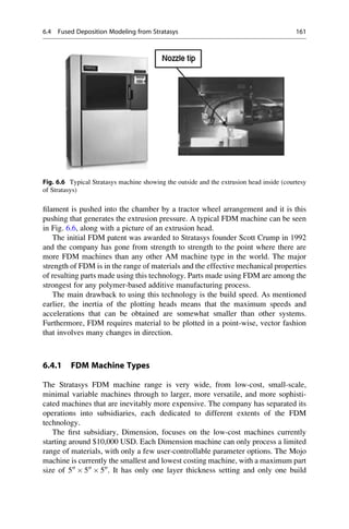
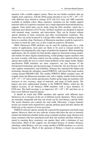
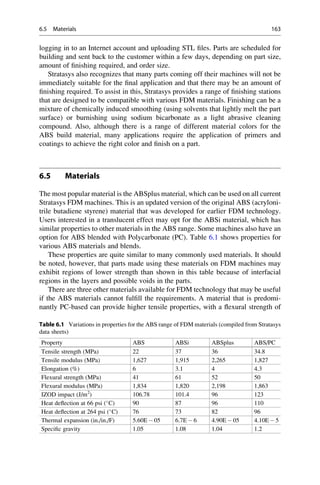
![6.7 Bioextrusion
Extrusion-based technology has a large variety of materials that can be processed. If
a material can be presented in a liquid form that can quickly solidify, then it is
suitable to this process. As mentioned earlier, the creation of this liquid can be
either through thermal processing of the material to create a melt, or by using some
form of chemical process where the material is in a gel form that can dry out or
chemically harden quickly. These techniques are useful for bioextrusion.
Bioextrusion is the process of creating biocompatible and/or biodegradable
components that are used to generate frameworks, commonly referred to as
“scaffolds,” that play host to animal cells for the formation of tissue (tissue
engineering). Such scaffolds should be porous, with micropores that allow cell
adhesion and macropores that provide space for cells to grow.
There are a few commercial bioextrusion systems, like the modified FDM
process used by Osteopore [8] to create scaffolds to assist in primarily head trauma
recovery. This machine uses a conventional FDM-like process with settings for a
proprietary material, based on the biocompatible polymer, polycaprolactone (PCL).
Most tissue engineering is still, however, in research form; investigating many
aspects of the process, including material choice, structural strength of scaffolds,
coatings, biocompatibility, and effectiveness within various clinical scenarios.
Many systems are in fact developed in-house to match the specific interests of the
researchers. There are however a small number of systems that are also available
commercially to research labs.
6.7.1 Gel Formation
One common method of creating scaffolds is to use hydrogels. These are polymers
that are water insoluble but can be dispersed in water. Hydrogels can therefore be
extruded in a jelly-like form. Following extrusion, the water can be removed and a
solid, porous media remains. Such a media can be very biocompatible and condu-
cive to cell growth with low toxicity levels. Hydrogels can be based on naturally
occurring polymers or synthetic polymers. The natural polymers are perhaps more
biocompatible whereas the synthetic ones are stronger. Synthetic hydrogels are
rarely used in tissue engineering, however, because of the use of toxic reagents.
Overall, use of hydrogels results in weak scaffolds that may be useful for soft tissue
growth.
6.7.2 Melt Extrusion
Where stronger scaffolds are required, like when used to generate bony tissue, melt
extrusion seems to be the process of choice. FDM can be used, but there are some
difficulties in using this approach. In particular, FDM is somewhat unsuitable
because of the expense of the materials. Biocompatible polymers suitable for tissue
166 6 Extrusion-Based Systems](https://image.slidesharecdn.com/1-230308091212-68402451/85/1-Additive-manufacturing-pdf-186-320.jpg)
![engineering are synthesized in relatively small quantities and are therefore only
provided at high cost. Furthermore, the polymers often need to be mixed with other
materials, like ceramics, that can seriously affect the flow characteristics, causing
the material to behave in a non-Newtonian manner. Extrusion using FDM requires
the material to be constructed in filament form that is pushed through the system by
a pinch roller feed mechanism. This mechanism may not provide sufficient pressure
at the nozzle tip, however, and so many of the experimental systems use screw feed,
similar to conventional injection molding and extrusion technology. Screw feed
systems benefit from being able to feed small amounts of pellet-based feedstock,
enabling one to work with a small material volume.
In addition to their layer-wise photopolymerization machines, Envisiontec [9]
has also developed the 3D-Bioplotter system (see Fig. 6.7). This system is an
extrusion-based, screw feeding technology that is designed specifically for
biopolymers. Lower temperature polymers can be extruded using a compressed
gas feed, instead of a screw extruder, which results in a much simpler mechanism.
Much of the system uses nonreactive stainless steel and the machine itself has a
small build envelope and software specifically aimed at scaffold fabrication. The
melt chamber is sealed apart from the nozzle, with a compressed air feed to assist
the screw extrusion process. The system uses one extrusion head at a time, with a
carousel feeder so that extruders can be swapped at any time during the process.
This is particularly useful since most tissue engineering research focuses on build-
ing scaffolds with different regions made from different materials. Build
parameters can be set for a variety of materials with control over the chamber
temperature, feed rate, and plotting speed to provide users with a versatile platform
for tissue engineering research.
It should be noted that tissue engineering is an extremely complex research area
and the construction of physical scaffolds is just the starting point. This approach
may result in scaffolds that are comparatively strong compared with hydrogel-
based scaffolds, but they may fail in terms of biocompatibility and bio-toxicity. To
overcome some of these shortcomings, a significant amount of post-processing is
required.
Fig. 6.7 The Envisiontec 3D
Bioplotter system (note the
multiple head changing
system on the right-hand
side)
6.7 Bioextrusion 167](https://image.slidesharecdn.com/1-230308091212-68402451/85/1-Additive-manufacturing-pdf-187-320.jpg)
![6.7.3 Scaffold Architectures
One of the major limitations with extrusion-based systems for conventional
manufacturing applications relates to the diameter of the nozzle. For tissue engi-
neering, however, this is not such a limitation. Scaffolds are generally built up so
that roads are separated by a set distance so that the scaffold can have a specific
macro porosity. In fact, the aim is to produce scaffolds that are as strong as possible
but with as much porosity as possible. The greater the porosity, the more space there
is for cells to grow. Scaffolds with greater than 66 % porosity are common.
Sometimes, therefore, it may be better to have a thicker nozzle to build stronger
scaffold struts. The spacing between these struts can be used to determine the
scaffold porosity.
The most effective geometry for scaffolds has yet to be determined. For many
studies scaffolds with a simple 0
and 90
orthogonal crossover pattern may be
sufficient. More complex patterns vary the number of crossovers and their separa-
tion. Examples of typical patterns can be seen in Fig. 6.8. Much of the studies
involve finding out how cells proliferate in these different scaffold architectures and
are usually carried out using bioreactors for in vitro (noninvasive) experiments. As
such, samples are usually quite small and often cut from a larger scaffold structure.
It is anticipated that it will become commonplace for experiments to be carried out
using samples that are as large and complex in shape as the bones they are designed
to replace and that are implanted in animal or human subjects. Many more funda-
mental questions must be answered, however, before this becomes common.
6.8 Other Systems
Although Stratasys owns most of the patents on FDM and similar heat-based
extrusion technology, there are a number of other such systems commercially
available. The majority of these systems can be purchased only in China, until
the expiration of Stratasys’ patents. The most successful and well-known system is
available from the Beijing Yinhua company. Most of these competing FDM
Fig. 6.8 Different scaffold designs showing a porous structure, with an actual image of a scaffold
created using a bioextrusion system [10]
168 6 Extrusion-Based Systems](https://image.slidesharecdn.com/1-230308091212-68402451/85/1-Additive-manufacturing-pdf-188-320.jpg)
![machines utilize a screw extrusion system that are fed using powder or pellet feed
rather than continuous filaments.
6.8.1 Contour Crafting
In normal additive manufacturing, layers are considered as 2D shapes extruded
linearly in the third dimension. Thicker layers result in lower part precision,
particularly where there are slopes or curves in the vertical direction. A major
innovative twist on the extrusion-based approach can be found in the Contour
Crafting technology developed by Prof. B. Khoshnevis and his team at the Univer-
sity of Southern California [11]. Taking the principle mentioned above that the
exterior surface is the most critical in terms of meeting precision requirements, this
research team has developed a method to smooth the surface with a scraping tool.
This is similar to how artisans shape clay pottery and/or concrete using trowels. By
contouring the layers as they are being deposited using the scraping tool to
interpolate between these layers, very thick layers can be made that still replicate
the intended geometry well.
Using this technique it is conceptually possible to fabricate extremely large
objects very quickly compared with other additive processes, since the exterior
precision is no longer determined solely by the layer thickness. The scraper tool
need not be a straight edge and can indeed be somewhat reconfigurable by posi-
tioning different parts of the tool in different regions or by using multiple passes. To
illustrate this advantage the team is in fact developing technology that can produce
full-sized buildings using a mixture of the Contour Crafting process and robotic
assembly (see Fig. 6.9).
6.8.2 Nonplanar Systems
There have been a few attempts at developing AM technology that does not use
stratified, planar layers. The most notable projects are Shaped Deposition Manu-
facture (SDM), Ballistic Particle Manufacture (BPM), and Curved Laminated
Object Manufacture (Curved LOM). The Curved LOM [12] process in particular
aims at using fiber-reinforced composite materials, sandwiched together for the
purposes of making tough-shelled components like nose cones for aircraft using
carbon fiber and armored clothing using Kevlar. To work properly, the layers of
material must conform to the shape of the part being designed. If edges of laminates
are exposed then they can easily come loose by applying shear forces. The Curved
LOM process demonstrated feasibility but also quickly became a very complex
system that required conformable robotic handling equipment and high powered
laser cutting for the laminates.
6.8 Other Systems 169](https://image.slidesharecdn.com/1-230308091212-68402451/85/1-Additive-manufacturing-pdf-189-320.jpg)
![It is possible to use short fibers mixed with polymer resins in FDM. Fibers can be
extruded so long as the diameter and length of the fibers are small enough to prevent
clogging of the nozzles. Like Curved LOM, it is somewhat pointless to use such a
material in FDM if the layers are aligned with the build plane. However, if the
layers were aligned according to the outer layer of the part, then it may be useful.
Parts cannot be built using a flat layer approach, in this case, and thus process
planning for complex geometries becomes problematic. However, certain parts that
require surface toughness can benefit from this nonplanar approach [13].
Fig. 6.9 Contour Crafting technology, developed at USC, showing scraping device and large-
scale machine
170 6 Extrusion-Based Systems](https://image.slidesharecdn.com/1-230308091212-68402451/85/1-Additive-manufacturing-pdf-190-320.jpg)
![6.8.3 FDM of Ceramics
Another possible application of FDM is to develop ceramic part fabrication pro-
cesses. In particular, FDM can be used to extrude ceramic pastes that can quickly
solidify. The resulting parts can be fired using a high-temperature furnace to fuse
and densify the ceramic particles. Resulting parts can have very good properties
with the geometric complexity characteristics of AM processes. Other AM pro-
cesses have also been used to create ceramic composites, but most work using FDM
came out of Rutgers University in the USA [14].
6.8.4 Reprap and Fab@home
The basic FDM process is quite simple; and this can be illustrated by the develop-
ment of two systems that are extremely low cost and capable of being constructed
using minimal tools.
The Reprap project [15] is essentially an experiment in open source technology.
The initial idea was developed by a group at the University of Bath in the UK and
designs and ideas are being developed by a number of enthusiasts worldwide. One
concept being considered is that a machine is capable of producing components for
future machines, testing some of the theories of von Neumann on self-replicating
machines. A large number of design variants exist, some using cold-cure resins but
most using a thermal extrusion head, but all are essentially variants of the FDM
process, as illustrated by one of these designs shown in Fig. 6.10.
Another project that aims at low-cost FDM technology is the Fab@home
concept. This uses a frame constructed from laser-cut polymer sheets, assembled
like a 3D jigsaw. Low-cost stepper motors and drives commonly found in ink-jet
printers are used for positioning and the extrusion head is normally a compressed-
air-fed syringe that contains a variety of cold-cure materials. The Fab@home
designs can be obtained free of charge and kits can be obtained for assembly at a
very low cost.
Both of these approaches have inspired a variety of enthusiasts to develop their
ideas. Some have focused on improving the designs so that they may be more robust
or more versatile. Others have developed software routines that explore things like
scanning patterns, more precise control, etc. Yet other enthusiasts have developed
new potential applications for this technology, most notably using multiple
materials that have unusual chemical or physical behavior. The Fab@home tech-
nology has, for example, been used to develop 3D batteries and actuators. Some
users have even experimented with chocolate to create edible sculptures.
This development of entry-level AM technology has sparked a 3D Printing
revolution that has attracted huge amounts of media attention and brought it into
the public domain. This explosion in interest is covered in more detail in a later
chapter of this book.
6.8 Other Systems 171](https://image.slidesharecdn.com/1-230308091212-68402451/85/1-Additive-manufacturing-pdf-191-320.jpg)
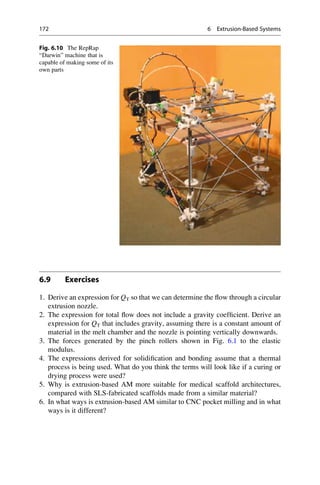

![commercialized by companies such as HP and Canon. Le [1] provides a thorough
review of the historical development of the inkjet printing industry.
Printing as a three-dimensional building method was first demonstrated in the
1980s with patents related to the development of Ballistic Particle Manufacturing,
which involved simple deposition of “particles” of material onto an article [2]. The
first commercially successful technology was the ModelMaker from Sanders Pro-
totype (now Solidscape), introduced in 1994, which printed a basic wax material
that was heated to liquid state [3]. In 1996, 3D Systems joined the competition with
the introduction of the Actua 2100, another wax-based printing machine. The Actua
was revised in 1999 and marketed as the ThermoJet [3]. In 2001, Sanders Design
International briefly entered the market with its Rapid ToolMaker, but was quickly
restrained due to intellectual property conflicts with Solidscape [3]. It is notable that
all of these members of the first generation of RP printing machines relied on heated
waxy thermoplastics as their build material; they are therefore most appropriate for
concept modeling and investment casting patterns.
More recently, the focus of development has been on the deposition of acrylate
photopolymer, wherein droplets of liquid monomer are formed and then exposed to
ultraviolet light to promote polymerization. The reliance upon photopolymerization
is similar to that in stereolithography, but other process challenges are significantly
different. The leading edge of this second wave of machines arrived on the market
with the Quadra from Objet Geometries of Israel in 2000, followed quickly by the
revised QuadraTempo in 2001. Both machines jetted a photopolymer using print
heads with over 1,500 nozzles [3]. In 2003, 3D Systems launched a competing
technology with its InVision 3D printer. Multi-Jet Modeling, the printing system
used in this machine, was actually an extension of the technology developed with
the ThermoJet line [3], despite the change in material solidification strategy. The
companies continue to innovate, as will be discussed in the next sections.
7.2 Materials for Material Jetting
While industry players have so far introduced printing machines that use waxy
polymers and acrylic photopolymers exclusively, research groups around the world
have experimented with the potential for printing machines that could build in those
and other materials. Among those materials most studied and most promising for
future applications are polymers, ceramics, and metals. In addition to the commer-
cially available materials, this section highlights achievements in related research
areas.
For common droplet formation methods, the maximum printable viscosity
threshold is generally considered to be in the range of 20–40 centipoise (cP) at
the printing temperature [4–6]. An equivalent unit of measure is the milli-Pascal-
second, denoted mPa s if SI units are preferred. To facilitate jetting, materials that
are solid at room temperature must be heated so that they liquefy. For high viscosity
fluids, the viscosity of the fluid must be lowered to enable jetting. The most
common practices are to use heat or solvents or other low viscosity components
176 7 Material Jetting](https://image.slidesharecdn.com/1-230308091212-68402451/85/1-Additive-manufacturing-pdf-195-320.jpg)
![in the fluid. In addition to these methods, it is also possible that in some polymer
deposition cases shear thinning might occur, dependent upon the material or
solution in use; drop-on-demand (DOD) printers are expected to produce strain
rates of 103
–104
, which should be high enough to produce shear-thinning effects [4,
7]. While other factors such as liquid density or surface tension and print head or
nozzle design may affect the results, the limitation on viscosity quickly becomes the
most problematic aspect for droplet formation in material jetting.
7.2.1 Polymers
Polymers consist of an enormous class of materials, representing a wide range of
mechanical properties and applications. And although polymers are the only mate-
rial currently used in commercial AM machines, there seems to be relatively little
discussion on polymer inkjet production of macro three-dimensional structures in
the published scientific literature.
Gao and Sonin [8] present the first notable academic study of the deposition and
solidification of groups of molten polymer microdrops. They discuss findings
related to three modes of deposition: columnar, sweep (linear), and repeated
sweep (vertical walls). The two materials used in their investigations were a
candelilla wax and a microcrystalline petroleum wax, deposited in droplets
50 μm in diameter from a print head 3–5 mm from a cooled substrate. The authors
first consider the effects of droplet deposition frequency and cooling on columnar
formation. As would be expected, if the drops are deposited rapidly (50 Hz in this
case), the substrate on which they impinge is still at an elevated temperature,
reducing the solidification contact angle and resulting in ball-like depositions
instead of columns (Fig. 7.1a). Numerical analyses of the relevant characteristic
times of cooling are included. Gao and Sonin also consider horizontal deposition of
droplets and the subsequent formation of lines. They propose that smooth solid lines
will be formed only in a small range of droplet frequencies, dependent upon the
sweep speed, droplet size, and solidification contact angle (Fig. 7.1b). Finally, they
propose that wall-like deposition will involve a combination of the relevant aspects
from each of the above situations.
Reis et al. [9] also provide some discussion on the linear deposition of droplets.
They deposited molten Mobilwax paraffin wax with a heated print head from
SolidScape. They varied both the print head horizontal speed and the velocity of
droplet flight from the nozzle. For low droplet speeds, low sweep speeds created
discontinuous deposition and high sweep speeds created continuous lines
(Fig. 7.2a–c). High droplet impact speed led to splashing at high sweep speeds
and line bulges at low sweep speeds (Fig. 7.2d–f).
From these studies, it is clear that process variables such as print head speed,
droplet velocity, and droplet frequency affect the quality of the deposit. These
process variables vary depending upon the characteristics of the fluid being printed,
so some process development, or fine-tuning, is generally required when trying to
print a new material or develop a new printing technology.
7.2 Materials for Material Jetting 177](https://image.slidesharecdn.com/1-230308091212-68402451/85/1-Additive-manufacturing-pdf-196-320.jpg)
![Feng et al. [10] finally present a full system, based on a print head from
MicroFab Technologies Inc. that functions similarly to the commercially available
machines. It prints a wax material which is heated to 80
C, more than 10
past its
melting point, and deposits it in layers 13–60 μm thick. The deposition pattern is
controlled by varying the droplet size and velocity, as well as the pitch and hatch
500
Deposition frequency/Hz
200 100 50 30 20 15 10 7 0
/ (Hz)
235
330
340
375
470
690
935
1128
1428
1724
2000
2500
Fig. 7.1 (a) Columnar formation and (b) line formation as functions of droplet impingement
frequency [8]
Fig. 7.2 Results of varying sweep and impact speeds [9]
178 7 Material Jetting](https://image.slidesharecdn.com/1-230308091212-68402451/85/1-Additive-manufacturing-pdf-197-320.jpg)
![spacing of the lines produced. An example of the result, a 2.5-dimensional gear, is
presented in Fig. 7.3.
The earliest and most often used solution to the problem of high viscosity is to
heat the material until its viscosity drops to an acceptable point. As discussed in
Sect. 7.5, for example, commercial machines such as 3D Systems’ ThermoJet and
Solidscape’s T66 all print proprietary thermoplastics, which contain mixtures of
various waxes and polymers that are solid at ambient temperatures but convert to a
liquid phase at elevated printing temperatures [11]. In developing their hot melt
materials, for example, 3D Systems investigated various mixtures consisting of a
low shrinkage polymer resin, a low viscosity material such as paraffin wax, a
microcrystalline wax, a toughening polymer, and a small amount of plasticizer,
with the possible additions of antioxidants, coloring agents, or heat dissipating filler
[12]. These materials were formulated to have a viscosity of 18–25 cP and a surface
tension of 24–29 dyn/cm at the printing temperature of 130
C. De Gans et al. [13]
contend that they have used a micropipette optimized for polymer printing
applications that was able to print Newtonian fluids with viscosities up to 160 cP.
The most recent development in addressing the issues of viscosity is the use of
prepolymers in the fabrication of polymer parts. This is the method currently
employed by the two newest commercially available machine lines, as discussed
in Sect. 7.5. For example, 3D Systems investigated a series of UV-curable printing
materials, consisting of mixtures of high-molecular weight monomers and
oligomers such as urethane acrylate or methacrylate resins, urethane waxes, low
molecular weight monomers and oligomers such as acrylates or methacrylates that
function as diluents, a small amount of photoinitiators, and other additives such as
stabilizers, surfactants, pigments, or fillers [14, 15]. These materials also benefited
from the effects of hot melt deposition, as they were printed at a temperature of 70–
95
C, with melting points between 45 and 65
C. At the printing temperatures,
these materials had a viscosity of about 10–16 cP.
Fig. 7.3 Wax gear [10]
7.2 Materials for Material Jetting 179](https://image.slidesharecdn.com/1-230308091212-68402451/85/1-Additive-manufacturing-pdf-198-320.jpg)
![One problem encountered, and the reason that the printing temperatures cannot
be as high as those used in hot melt deposition, is that when kept in the heated state
for extended periods of time, the prepolymers begin to polymerize, raising the
viscosity and possibly clogging the nozzles when they are finally printed
[15]. Another complication is that the polymerization reaction, which occurs after
printing, must be carefully controlled to assure dimensional accuracy.
7.2.2 Ceramics
One significant advance in terms of direct printing for three-dimensional structures
has been achieved in the area of ceramic suspensions. As in the case of polymers,
studies have been conducted that investigate the basic effects of modifying sweep
speed, drop-to-drop spacing, substrate material, line spacing, and simple multilayer
forms in the deposition of ceramics [16]. These experiments were conducted with a
mixture of zirconia powder, solvent, and other additives, which was printed from a
62 μm nozzle onto substrates 6.5 mm away. The authors found that on substrates that
permitted substantial spreading of the deposited materials, neighboring drops would
merge to form single, larger shapes, whereas on other substrates the individual dots
would remain independent (see Fig. 7.4). In examples where multiple layers were
printed, the resulting deposition was uneven, with ridges and valleys throughout.
A sizable body of work has been amassed in which suspensions of alumina
particles are printed via a wax carrier [4] which is melted by the print head.
Suspensions of up to 40 % solids loading have been successfully deposited at
viscosities of 2.9–38.0 cP at a measurement temperature of 100
C; higher
concentrations of the suspended powder have resulted in prohibitively high
viscosities. Because this deposition method results in a part with only partial
ceramic density, the green part must be burnt out and sintered, resulting in a final
product which is 80 % dense but whose dimensions are subject to dramatic
shrinkage [17]. A part created in this manner is shown in Fig. 7.5.
Fig. 7.4 Droplets on two different substrates [16]
180 7 Material Jetting](https://image.slidesharecdn.com/1-230308091212-68402451/85/1-Additive-manufacturing-pdf-199-320.jpg)
![Similar attempts have been made with zirconia powder, using material with
14 % ceramic content by volume [18], with an example shown in Fig. 7.6, as well as
with PZT, up to 40 % ceramic particles by volume [19].
7.2.3 Metals
Much of the printing work related to metals has focused upon the use of printing for
electronics applications—formation of traces, connections, and soldering. Liu and
Orme [20] present an overview of the progress made in solder droplet deposition for
the electronics industry. Because solder has a low melting point, it is an obvious
choice as a material for printing. They reported use of droplets of 25–500 μm, with
Fig. 7.5 Sintered alumina
impeller [17]
Fig. 7.6 Sintered zirconia
vertical walls [18]
7.2 Materials for Material Jetting 181](https://image.slidesharecdn.com/1-230308091212-68402451/85/1-Additive-manufacturing-pdf-200-320.jpg)
![results such as the IC test board in Fig. 7.7, which has 70 μm droplets of Sn63/Pb37.
In related work, a solder was jetted whose viscosity was approximately 1.3 cP,
continuously jetted under a pressure of 138 kPa. Many of the results to which they
refer are those of researchers at MicroFab Technologies, who have also produced
solder forms such as 25 μm diameter columns.
There is, however, some work in true three-dimensional fabrication with metals.
Priest et al. [21] provide a survey of liquid metal printing technologies and history,
including alternative technologies employed and ongoing research initiatives.
Metals that had been printed included copper, aluminum, tin, various solders, and
mercury. One major challenge identified for depositing metals is that the melting
point of the material is often high enough to significantly damage components of
the printing system.
Orme et al. [22, 23] report on a process that uses droplets of Rose’s metal
(an alloy of bismuth, lead, and tin). They employ nozzles of diameter 25–150 μm
with resulting droplets of 47–283 μm. In specific cases, parts with porosity as low as
0.03 % were formed without post-processing, and the microstructure formed is
more uniform than that of standard casting. In discussion of this technology,
considerations of jet disturbance, aerodynamic travel, and thermal effects are all
presented.
Yamaguchi et al. [24, 25] used a piezoelectrically driven actuator to deposit
droplets of an alloy (Bi–Pb–Sn–Cd–In), whose melting point was 47
C. They
heated the material to 55
C and ejected it from nozzles 200 μm, 50 μm, and less
than 8 μm in diameter. As expected, the finer droplets created parts with better
resolution. The density, or “packing rate,” of some parts reached 98 %. Other
examples of fabricated parts are shown in Fig. 7.8.
Fig. 7.7 IC test board with solder droplets [20]
182 7 Material Jetting](https://image.slidesharecdn.com/1-230308091212-68402451/85/1-Additive-manufacturing-pdf-201-320.jpg)
![More recently, several research groups have demonstrated aluminum deposition
[26, 27]. In one example, near-net shape components, with fairly simple shapes,
have been formed from Al2024 alloy printed from a 100 μm orifice. In another
example, pressure pulses of argon gas in the range of 20–100 kPa were used to eject
droplets of molten aluminum at the rate of 1–5 drops per second. To achieve this,
the aluminum was melted at 750
C and the substrate to 300
C. The nozzle orifice
used was 0.3 mm in diameter, with a resulting droplet size of 200–500 μm and a
deposited line of width 1.00 mm and thickness 0.17 mm. The final product was a
near-net shape part of density up to 92 %.
As these examples have shown, printing is well on its way to becoming a viable
process for three-dimensional prototyping and manufacturing. While industry has
only barely begun to use printing in this arena, the economic and efficiency
advantages that printing provide ensure that it will be pursued extensively in the
future. Researchers in academia have expanded the use of printing to materials such
as ceramics and metals, thus providing additional prospective applications for the
technology. Despite its great potential, however, the growth of printing has been
hampered significantly by technical challenges inherent to the printing process.
These challenges and possible solutions are investigated in subsequent sections.
7.2.4 Solution- and Dispersion-Based Deposition
As hot melt deposition has very specific requirements for the material properties of
what is printed, many current applications have turned to solution- or dispersion-
based deposition. This allows the delivery of solids or high-molecular weight
polymers in a carrier liquid of viscosity low enough to be successfully printed.
De Gans et al. [5] provided a review of a number of polymeric applications in which
this strategy is employed.
A number of investigators have used solution and dispersion techniques in
accurate deposition of very small amounts of polymer in thin layers for mesoscale
applications, such as polymer light-emitting displays, electronic components, and
surface coatings and masks. For example, Shimoda et al. [28] present a technique to
develop light-emitting polymer diode displays using inkjet deposition of conduc-
tive polymers. Three different electroluminescent polymers (polyfluorine and two
Fig. 7.8 Examples of parts fabricated with metal printing [25]
7.2 Materials for Material Jetting 183](https://image.slidesharecdn.com/1-230308091212-68402451/85/1-Additive-manufacturing-pdf-202-320.jpg)
![derivatives) were printed in organic solvents at 1–2 wt%. As another example, De
Gans et al. [5] report a number of other results related to the creation of polymer
light-emitting displays: a precursor of poly( p-phenylene vinylene) (PPV) was
printed as a 0.3 wt% solution; and PPV derivatives were printed in 0.5–2.0 wt%
solutions in solvents such as tetraline, anisole, and o-xylene. Such low weight
percentages are typical.
In deposition of ceramics, the use of a low viscosity carrier is also a popular
approach. Tay and Edirisinghe [16], for example, used ceramic powder dispersed in
industrial methylated spirit with dispersant, binder, and plasticizer additives
resulting in a material that was 4.5 % zirconia by volume. The resulting material
had a viscosity of 3.0 cP at 20
C and a shear rate of 1,000 s1
. Zhao et al. [29]
tested various combinations of zirconia and wax carried in octane and isopropyl
alcohol, with a dispersant added to reduce sedimentation. The viscosities of these
materials were 0.6–2.9 cP at 25
C; the one finally selected was 14.2 % zirconia by
volume.
Despite the success of solution and dispersion deposition for these specific
applications, however, there are some serious drawbacks, especially in considering
the potential for building complex, large, 3D components. The low concentrations
of polymer and solid used in the solutions and dispersions will restrict the total
amount of material that can be deposited. Additionally, it can be difficult to control
the deposition pattern of this material within the area of the droplet’s impact.
Shimoda et al. [28], among others, report the formation of rings of deposited
material around the edge of the droplet. They attribute this to the fact that the
contact line of the drying drop is pinned on the substrate. As the liquid evaporates
from the edges, it is replenished from the interior, carrying the solutes to the edge.
They contend that this effect can be mitigated by control of the droplet drying
conditions.
Another difficulty with solutions or dispersions, especially those based on
volatile solvents, is that use of these materials can result in precipitations forming
in the nozzle after a very short period of time [13], which can clog the nozzle,
making deposition unreliable or impossible.
7.3 Material Processing Fundamentals
7.3.1 Technical Challenges of MJ
As evidenced by the industry and research applications discussed in the previous
section, material jetting already has a strong foothold in terms of becoming a
successful AM technology. There are, however, some serious technical
shortcomings that have prevented its development from further growth. To identify
and address those problems, the relevant phenomena and strategic approaches taken
by its developers must be understood. In the next two sections, the technical
challenges of the printing process are outlined, the most important of its limitations
184 7 Material Jetting](https://image.slidesharecdn.com/1-230308091212-68402451/85/1-Additive-manufacturing-pdf-203-320.jpg)
![relevant to the deposition of functional polymers are identified, and how those
limitations are currently addressed is summarized.
Jetting for three-dimensional fabrication is an extremely complex process, with
challenging technical issues throughout. The first of these challenges is formulation
of the liquid material. If the material is not in liquid form to begin with, this may
mean suspending particles in a carrier liquid, dissolving materials in a solvent,
melting a solid polymer, or mixing a formulation of monomer or prepolymer with a
polymerization initiator. In many cases, other substances such as surfactants are
added to the liquid to attain acceptable characteristics. Entire industries are devoted
to the mixture of inks for two-dimensional printing, and it is reasonable to assume
that in the future this will also be the case for three-dimensional fabrication.
The second hurdle to overcome is droplet formation. To use inkjet deposition
methods, the material must be converted from a continuous volume of liquid into a
number of small discrete droplets. This function is often dependent upon a finely
tuned relationship between the material being printed, the hardware involved, and
the process parameters; a number of methods of achieving droplet formation are
discussed in this section. Small changes to the material, such as the addition of tiny
particles [30], can dramatically change its droplet forming behavior as well, as can
changes to the physical setup.
A third challenge is control of the deposition of these droplets; this involves
issues of droplet flight path, impact, and substrate wetting or interaction [31–35]. In
printing processes, either the print head or the substrate is usually moving, so the
calculation of the trajectory of the droplets must take this issue into account. In
addition to the location of the droplets’ arrival, droplet velocity and size will also
affect the deposition characteristics and must be measured and controlled via nozzle
design and operation [36]. The quality of the impacted droplet must also be
controlled: if smaller droplets, called satellites, break off from the main droplet
during flight, then the deposited material will be spread over a larger area than
intended and the deposition will not have well-defined boundaries. In the same way,
if the droplet splashes on impact, forming what is called a “crown,” similar results
will occur [37]. All of the effects will negatively impact the print quality of the
printed material.
Concurrently, the conversion of the liquid material droplets to solid geometry
must be carefully controlled; as discussed in Sect. 7.2, material jetting relies on a
phase change of the printed material. Examples of phase change modes employed
in existing printing technologies are: solidification of a melted material (e.g., wax,
solder), evaporation of the liquid portion of a solution (e.g., some ceramic
approaches), and curing of a photopolymer (e.g., Objet, ProJet machines) or other
chemical reactions. The phase change must occur either during droplet flight or
soon after impact; the time and place of this conversion will also affect the droplet’s
interaction with the substrate [38, 39] and the final deposition created. To further
complicate the matter, drops may solidify nonuniformly, creating warpage and
other undesirable results [40].
An additional challenge is to control the deposition of droplets on top
of previously deposited layers, rather than only upon the initial substrate
7.3 Material Processing Fundamentals 185](https://image.slidesharecdn.com/1-230308091212-68402451/85/1-Additive-manufacturing-pdf-204-320.jpg)
![[8, 16]. The droplets will interact differently, for example, with a metal plate
substrate than with a surface of previously printed wax droplets. To create substan-
tive three-dimensional parts, each layer deposited must be fully bound to the
previous layer to prevent delamination, but must not damage that layer while
being created. Commercially available machines tend to approach this problem by
employing devices that plane or otherwise smooth the surface periodically [40–42].
Operational considerations also pose a challenge in process planning for MJ. For
example, because nozzles are so small, they often clog, preventing droplets from
exiting. Much attention has been given to monitoring and maintaining nozzle
performance during operation [40]. Most machines currently in use go through
purge and cleaning cycles during their builds to keep as many nozzles open as
possible; they may also wipe the nozzles periodically [41]. Some machines may
also employ complex sensing systems to identify and compensate for
malfunctioning or inconsistent nozzles [43, 44]. In addition, many machines,
including all commercial AM machines, have replaceable nozzles in case of
permanent blockage.
Finally, to achieve the best print resolution, it is advantageous to produce many
small droplets very close together. However, this requires high nozzle density in the
print head, which is unattainable for many nozzle manufacturing processes. An
alternative to nozzle density is to make multiple passes over the same area,
effectively using process planning instead of hardware to create the desired effect
[41]. Even in cases where high nozzle density is possible, however, problems arise
due to crosstalk—basically an “overlapping” of the thermal or pressure differentials
used to drive adjacent nozzles.
In approaching a printing process, these numerous challenges must in some
sense be addressed sequentially: flight pattern cannot be studied until droplets are
formed and layering cannot be investigated until deposition of single droplets is
controlled. In terms of functional polymer deposition, the challenge of material
preparation has effectively been addressed; numerous polymer resins and mixtures
already exist. It is the second challenge—droplet formation—that is therefore the
current limiting factor in deposition of these materials. To understand these
limitations, Sect. 7.3.2 reviews the dynamic processes that are currently used to
form droplets and Sect. 7.2 considered necessary methods of modifying the jetting
material for use with those processes.
7.3.2 Droplet Formation Technologies
Over the time that two-dimensional inkjet printing has evolved, a number of
methods for creating and expelling droplets have been developed. The main
distinction in categorizing the most common of technologies refers to the possible
modes of expulsion: continuous stream (CS) and DOD. This distinction refers to the
form in which the liquid exits the nozzle—as either a continuous column of liquid
or as discrete droplets. Figure 7.9 shows the distinction between continuous (left)
and DOD (right) formations.
186 7 Material Jetting](https://image.slidesharecdn.com/1-230308091212-68402451/85/1-Additive-manufacturing-pdf-205-320.jpg)
![7.3.3 Continuous Mode
In CS mode, a steady pressure is applied to the fluid reservoir, causing a pressurized
column of fluid to be ejected from the nozzle. After departing the nozzle, this
stream breaks into droplets due to Rayleigh instability. The breakup can be made
more consistent by vibrating, perturbing, or modulating the jet at a fixed frequency
close to the spontaneous droplet formation rate, in which case the droplet formation
process is synchronized with the forced vibration, and ink droplets of uniform mass
are ejected [45]. Because droplets are produced at constant intervals, their deposi-
tion must be controlled after they separate from the jet. To achieve this, they are
introduced to a charging field and thus attain an electrostatic charge. These charged
particles then pass through a deflection field, which directs the particles to their
desired destinations—either a location on the substrate or a container of material to
be recycled or disposed. Figure 7.10 shows a schematic of the function of this type
of binary deflection continuous system.
An advantage of CS deposition is the high throughput rate; it has therefore seen
widespread use in applications such as food and pharmaceutical labeling [5]. Two
major constraints related to this method of droplet formation are, however, that the
materials must be able to carry a charge and that the fluid deflected into the catcher
must be either disposed of or reprocessed, causing problems in cases where the fluid
is costly or where waste management is an issue.
In terms of droplets formed, commercially available systems typically generate
droplets that are about 150 μm in diameter at a rate of 80–100 kHz, but frequencies
of up to 1 MHz and droplet sizes ranging from 6 μm (10 fL) to 1 mm (0.5 μL) have
been reported [46]. It has also been shown that, in general, droplets formed from
continuous jets are almost twice the diameter of the undisturbed jet [47].
Fig. 7.9 Continuous (left)
and drop-on-demand (right)
deposition [46]
7.3 Material Processing Fundamentals 187](https://image.slidesharecdn.com/1-230308091212-68402451/85/1-Additive-manufacturing-pdf-206-320.jpg)
![A few investigators of three-dimensional deposition have opted to use continu-
ous printing methods. Blazdell et al. [48] used a continuous printer from Biodot,
which was modulated at 66 kHz while ejecting ceramic ink from 50 and 75 μm
nozzles. They used 280 kPa of air pressure. Blazdell [49] reports later results in
which this Biodot system was modulated at 64 kHz, using a 60 μm nozzle that was
also 60 μm in length. For much of the development of the 3D Printing binder jetting
process, CS deposition was used. At present, the commercial machines based on
3DP (from 3D Systems and Ex One) use standard DOD print heads. In metal
fabrication, Tseng et al. [50] used a continuous jet in depositing their solder
alloy, which had a viscosity of about 2 cP at the printing temperature. Orme
et al. [22, 23] also report the use of an unspecified continuous system in deposition
of solders and metals.
7.3.4 DOD Mode
In DOD mode, in contrast, individual droplets are produced directly from the
nozzle. Droplets are formed only when individual pressure pulses in the nozzle
cause the fluid to be expelled; these pressure pulses are created at specific times by
thermal, electrostatic, piezoelectric, acoustic, or other actuators [1]. Figure 7.11
shows the basic functions of a DOD setup. Liu and Orme [20] assert that DOD
methods can deposit droplets of 25–120 μm at a rate of 0–2,000 drops per second.
In the current DOD printing industry, thermal (bubble-jet) and piezoelectric
actuator technologies dominate; these are shown in Fig. 7.12. Thermal actuators
Drive
Signal
Fluid
Supply/
Pump
Charge
Driver
Deflection
Plates
Droplet
Catcher
Substrate
High
Voltage
Actuator
Fig. 7.10 Binary deflection
continuous printing [46]
188 7 Material Jetting](https://image.slidesharecdn.com/1-230308091212-68402451/85/1-Additive-manufacturing-pdf-207-320.jpg)
![Drive
Signal
Fluid
Supply
Actuator
Actuator
Pulse
Train
Substrate motion
Fig. 7.11 Schematic of
drop-on-demand printing
system [46]
Fig. 7.12 Thermal (top) and piezoelectric (bottom) DOD ejection
7.3 Material Processing Fundamentals 189](https://image.slidesharecdn.com/1-230308091212-68402451/85/1-Additive-manufacturing-pdf-208-320.jpg)
![rely on a resistor to heat the liquid within a reservoir until a bubble expands in it,
forcing a droplet out of the nozzle. Piezoelectric actuators rely upon the deforma-
tion of a piezoelectric element to reduce the volume of the liquid reservoir, which
causes a droplet to be ejected. As noted by Basaran [51], the waveforms employed
in piezoelectrically driven DOD systems can vary from simple positive square
waves to complex negative–positive–negative waves in which the amplitude,
duration, and other parameters are carefully modulated to create the droplets as
desired.
In their review of polymer deposition, De Gans et al. [5] assert that DOD is the
preferable method for all applications that they discuss due to its smaller drop size
(often of diameter similar to the orifice) and higher placement accuracy in compar-
ison to CS methods. They further argue that piezoelectric DOD is more widely
applicable than thermal because it does not rely on the formation of a vapor bubble
or on heating that can damage sensitive materials.
The preference for piezoelectrically driven DOD printing is reflected in the
number of investigators who use and study such setups. For example, Gao and
Sonin [8] use this technology to deposit 50 μm droplets of two waxes, whose
viscosity at 100
C is about 16 cP. Sirringhaus et al. [52] and Shimoda et al. [28]
both use piezoelectric DOD deposition for polymer solutions, as discussed in
Sect. 7.2.1. In ceramic deposition, Reis et al. [9] print mixtures with viscosities
6.5 and 14.5 cP at 100
C and frequencies of 6–20 kHz. Yamaguchi et al. [24, 25]
also used a piezoelectrically driven DOD device at frequencies up to 20 Hz in the
deposition of metal droplets. Similarly, the solder droplets on the circuit board in
Fig. 7.7 were also deposited with a DOD system.
At present, all commercial AM printing machines use DOD print heads, gener-
ally from a major manufacturer of printers or printing technologies. Such
companies include Hewlett-Packard, Canon, Dimatix, Konica-Minolta, and Xaar.
7.3.5 Other Droplet Formation Methods
Aside from the standard CS and DOD methods, other technologies have been
experimentally investigated but have not enjoyed widespread use in industry
applications. Liquid spark jetting, a relative of thermal printing, relies on an
electrical spark discharge instead of a resistor to form a gas bubble in the reservoir
[45, 52]. The electrohydrodynamic inkjet employs an extremely powerful electric
field to pull a meniscus and, under very specific conditions, droplets from a
pressure-controlled capillary tube; these droplets are significantly smaller than the
tube from which they emanate. Electro-rheological fluid jetting uses an ink whose
properties change under high electric fields; the fluid flows only when the electric
field is turned off [53]. In their flextensional ultrasound droplet ejectors, Percin and
Khuri-Yakub [54] demonstrate both DOD and continuous droplet formation with a
system in which a plate containing the nozzle orifice acts as the actuator, vibrating
at resonant frequencies and forming droplets by creating capillary waves on the
liquid surface as well as an increased pressure in the liquid. Focused acoustic beam
190 7 Material Jetting](https://image.slidesharecdn.com/1-230308091212-68402451/85/1-Additive-manufacturing-pdf-209-320.jpg)
![ejection uses a lens to focus an ultrasound beam onto the free surface of a fluid,
using the acoustic pressure transient generated by the focused tone burst to eject a
fluid droplet [55]. Meacham et al. extended this work [56] to develop an inexpen-
sive ultrasonic droplet generator and developed a fundamental understanding of its
droplet formation mechanisms [57]. These ultrasonic droplet generators show
promise in ejecting viscous polymers [58]. Fukumoto et al. [59] present a variant
technology in which ultrasonic waves are focused onto the surface of the liquid,
forming surface waves that eventually break off into a mist of small droplets.
Overviews of these various droplet formation methods are given by Lee [53] and
Basaran [51].
Summary: While the general challenges of material jetting for three-dimensional
fabrication are identified, there are many aspects that are not well or fully under-
stood. Open research questions abound in almost all stages of the printing process—
droplet formation, deposition control, and multilayer accumulation. For the case of
polymer jetting, the most appropriate limitation to address is that of droplet
formation. Because systems developed for inviscid materials are being used for
these applications, numerous accommodations and limitations currently exist; users
commonly handle this by modifying the materials to fit the requirements of the
existing hardware. However, if the method of droplet formulation could be
modified instead, this might allow the deposition of a wider range of materials. A
recently developed acoustic focusing ultrasonic droplet generator, under investiga-
tion at Georgia Institute of Technology, employs a strategy different from those of
existing technologies, which may provide the capabilities to fulfill this need [60].
7.4 MJ Process Modeling
Conservation of energy concepts provides an appropriate context for investigating
droplet generation mechanisms for printing. Essentially, the energy imparted by the
actuation method to the liquid must be sufficient to balance three requirements:
fluid flow losses, surface energy, and kinetic energy. The losses originate from a
conversion of kinetic energy to thermal energy due to the viscosity of the fluid
within the nozzle; this conversion can be thought of as a result of internal friction of
the liquid. The surface energy requirement is the additional energy needed to form
the free surface of the droplet or jet. Finally, the resulting droplet or jet must still
retain enough kinetic energy to propel the liquid from the nozzle towards the
substrate. This energy conservation can be summarized as
Eimparted ¼ Eloss þ Esurface þ Ekinetic ð7:1Þ
The conservation law can be considered in the form of actual energy calculations
or in the form of pressure, or energy per unit volume, calculations. For example,
Sweet used the following approximation for the gauge pressure required in the
reservoir of a continuous jetting system [61]:
7.4 MJ Process Modeling 191](https://image.slidesharecdn.com/1-230308091212-68402451/85/1-Additive-manufacturing-pdf-210-320.jpg)
![Δp ¼ 32μd2
j vj
Z l2
l1
dl
d4
n
þ
2σ
dj
þ
ρv2
j
2
ð7:2Þ
where, Δp is the total gauge pressure required, μ is the dynamic viscosity of the
liquid, ρ is the liquid’s density, σ is the liquid’s surface tension, dj is the diameter of
the resultant jet, dn is the inner diameter of the nozzle or supply tubing, vj is the
velocity of the resultant jet, and l is the length of the nozzle or supply tubing. The
first term on the right of (7.2) is an approximation of the pressure loss due to viscous
friction within the nozzle and supply tubing. The second term is the internal
pressure of the jet due to surface tension and the third term is the pressure required
to provide the kinetic energy of the droplet or jet.
Energy conservation can also be thought of as a balance among the effects before
the fluid crosses a boundary at the orifice of the nozzle and after it crosses that
boundary. Before the fluid leaves the nozzle, the positive effect of the driving
pressure gradient accelerates it, but energy losses due to viscous flow decelerate
it. The kinetic energy with which it leaves the nozzle must be enough to cover the
kinetic energy of the traveling fluid as well as the surface energy of the new free
surface.
As indicated earlier, actuation energy is typically in the form of heating (bubble-
jet) or vibration of a piezoelectric actuator. Various electrical energy waveforms
may be used for actuation. In any event, these are standard types of inputs and will
not be discussed further.
While the liquid to be ejected travels through the nozzle, before forming
droplets, its motion is governed by the standard equations for incompressible,
Newtonian fluids, as we are assuming these flows to be. The flow is fully described
by the Navier–Stokes and continuity equations; however, these equations are
difficult to solve analytically, so we will proceed with a simplification. The first
term on the right side of (7.2) takes advantage of one situation for which an
analytical solution is possible, that of steady, incompressible, laminar flow through
a straight circular tube of constant cross section. The solution is the Hagen–
Poiseuille law [62], which reflects the viscous losses due to wall effects:
Δp ¼
8Qμl
πr4σ
ð7:3Þ
where Q is the flow rate and r is the tube radius. Note that this expression is most
applicable when the nozzle is a long, narrow glass tube. However, it can also apply
when the fluid is viscous, as we will see shortly.
Another assumption made by using the Hagen–Poiseuille equation is that the
flow within the nozzle is fully developed. For the case of laminar flow in a
cylindrical pipe, the length of the entry region le where flow is not yet fully
developed is defined as 0.06 times the diameter of the pipe, multiplied by the
Reynolds number [62]:
192 7 Material Jetting](https://image.slidesharecdn.com/1-230308091212-68402451/85/1-Additive-manufacturing-pdf-211-320.jpg)
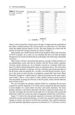
![increase linearly with viscosity, which again can be expected from (7.3). As
indicated, wall friction dominates for many printing condition. However, as nozzle
size increases, the surface tension of the fluid becomes more important. Also, as
viscosity increases, viscous losses become important, as viscous fluids can absorb
considerable acoustic energy. Regardless, this analysis provides good insight into
pressure variations under many typical printing conditions.
Fluid flows when printing are almost always laminar; i.e., the Reynolds number
is less than 2,100. As a reminder, the Reynolds number is
Re ¼
ρvr
μ
ð7:5Þ
Another dimensionless number of relevance in printing is the Weber number,
which describes the relative importance of a fluid’s inertia compared with its
surface tension. The expression for the Weber number is:
We ¼
ρv2
r
γ
ð7:6Þ
Several research groups have determined that a combination of the Reynolds and
Weber numbers is a particularly good indication of the potential for successful
printing of a fluid [17]. Specifically, if the ratio of the Reynolds number to the
square root of the Weber number has a value between 1 and 10, then it is likely that
ejection of the fluid will be successful. This condition will be called the “printing
indicator” and is
50
45
40
35
30
25
20
15
10
5
0
0 50 100 150
Viscosity [cP]
Pressure
[MPa]
200
dia = 0.02 mm
dia = 0.04 mm
dia = 0.06 mm
dia = 0.10 mm
Fig. 7.13 Pressure required to overcome wall friction for printing through nozzles of different
diameters
194 7 Material Jetting](https://image.slidesharecdn.com/1-230308091212-68402451/85/1-Additive-manufacturing-pdf-213-320.jpg)
![1
Re
We1=2
¼
ffiffiffiffiffiffiffi
ρrγ
p
μ
10 ð7:7Þ
The inverse of the printing indicator is another dimensionless number called the
Ohnsorge number, that relates viscous and surface tension forces. Note that values
of this ratio that are low indicate that flows are viscosity limited, while large values
indicate flows that are dominated by surface tension. The low value of 1 for the
printing indicator means that the maximum fluid viscosity should be between
20 and 40 cP.
Some examples of Reynolds numbers and printing indicators are given in
Table 7.2. For these results, the surface tension is 0.072 N/m, the density is
1,000 kg/m3
(same as water at room temperature), and droplet velocity is 1 m/s.
It is important to realize that the printing indicator is a guide, not a law to be
followed. Water is usually easy to print through most print heads, regardless of the
nozzle size. But the printing indicator predicts that water (with a viscosity of 1 cP)
should not be ejectable since its surface tension is too high. We will see in the next
section how materials can be modified in order to make printing feasible.
7.5 Material Jetting Machines
The three main companies involved in the development of the RP printing industry
are still the main players offering printing-based machines: Solidscape, 3D
Systems, and Stratasys (after their merger with Objet Geometries). Solidscape
sells the T66 and T612, both descendants of the previous ModelMaker line and
based upon the first-generation melted wax technique. Each of these machines
employs two single jets—one to deposit a thermoplastic part material and one to
deposit a waxy support material—to form layers 0.0005 in. thick [63]. It should be
noted that these machines also fly-cut layers after deposition to ensure that the layer
Table 7.2 Reynolds numbers and printing indicator values for some printing conditions
Nozzle diameter (mm) Viscosity (cP) Reynolds no. Printing indicator
0.02 1 20 37.9
10 2 3.79
40 0.5 0.949
100 0.2 0.379
0.05 1 50 60.0
10 5 6.00
40 1.25 1.50
100 0.5 0.600
0.1 1 100 84.9
10 10 8.49
40 2.5 2.12
100 1 0.849
7.5 Material Jetting Machines 195](https://image.slidesharecdn.com/1-230308091212-68402451/85/1-Additive-manufacturing-pdf-214-320.jpg)
![is flat for the subsequent layer. Because of the slow and accurate build style as well
as the waxy materials, these machines are often used to fabricate investment
castings for the jewelry and dentistry industries.
3D Systems and Stratasys offer machines using the ability to print and cure
acrylic photopolymers. Stratasys markets the Eden, Alaris, and Connex series of
printers. These machines print a number of different acrylic-based photopolymer
materials in 0.0006 in. layers from heads containing 1,536 individual nozzles,
resulting in rapid, line-wise deposition efficiency, as opposed to the slower,
point-wise approach used by Solidscape. Each photopolymer layer is cured by
ultraviolet light immediately as it is printed, producing fully cured models without
post-curing. Support structures are built in a gel-like material, which is removed by
hand and water jetting [64]. See Fig. 7.14 for an illustration of Stratasys’ Polyjet
system, which is employed in all Eden machines. The Connex line of machines
provides multimaterial capability. For several years, only two different
photopolymers could be printed at one time; however, by automatically adjusting
build styles, the machine can print up to 25 different effective materials by varying
the relative composition of the two photopolymers. Machines are emerging that
print increasing numbers of materials.
In competition with Stratasys, 3D Systems markets the ProJet printers, which
print layers 0.0016 in. thick using heads with hundreds of nozzles, half for part
material and half for support material [11]. Layers are then flashed with ultraviolet
light, which activates the photoinitiated polymerization. The ProJets are the third
generation of the Multi-Jet Modeling family from 3D Systems, following the
ThermoJet described above and the InVision series. A comparison of the machines
currently available is presented in Table 7.3.
Jetting Head X axis
Y axis
Z axis
UV Light
Fullcure M
(Model Material)
Fullcure S
(Support Material)
Build Tray
Fig. 7.14 Stratasys Polyjet build process [64]
196 7 Material Jetting](https://image.slidesharecdn.com/1-230308091212-68402451/85/1-Additive-manufacturing-pdf-215-320.jpg)
![Table
7.3
Commercially
available
printing-based
AM
machines
[11,
63,
64]
Company/product
Cost
(1000s)
Build
size
X
Y
Z
(mm)
Min.
layer
(mm)
Resolution
X,
Y
(dpi)
Material
Support
Solidscape
3Z
Studio
$25
152
152
51
0.01
8,000
8,000
Wax-like
Soluble
material
3Z
Pro
$46
152
152
102
0.01
8,000
8,000
”
”
3D
Systems
ProJet
3510
SD
$60
298
185
203
0.032
375
375
Acrylate
photopolymer
(AP)
”
ProJet
3510
HD
$78
298
185
203
0.029
750
750
AP
”
ProJet
3500
HDMax
$92
298
185
203
0.016
750
750
AP
”
ProJet
3500
CPXMax
$99
298
185
203
0.016
694
750
Wax-like
Wax
Stratasys
Objet
24
$20
240
200
150
–
–
AP
Gel-like
photopolymer
Eden
250
$60
255
252
200
0.028
600,
300
”
”
Eden
260V
$90
250
250
200
0.016
600,
600
”
”
Eden
500V
$170
490
390
200
0.016
600,
600
”
”
Connex500
$240
490
390
200
0.016
600,
600
”
”
Objet
1000
$500–700
1,000
800
500
0.016
600,
600
”
”
7.5 Material Jetting Machines 197](https://image.slidesharecdn.com/1-230308091212-68402451/85/1-Additive-manufacturing-pdf-216-320.jpg)
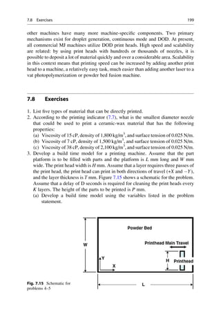
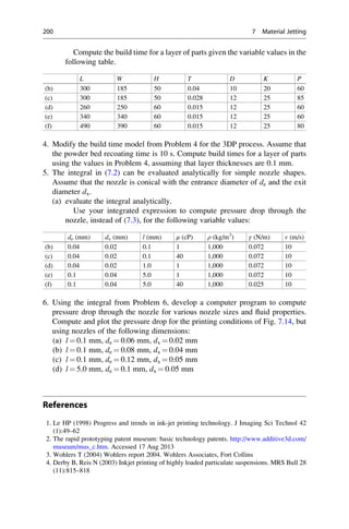
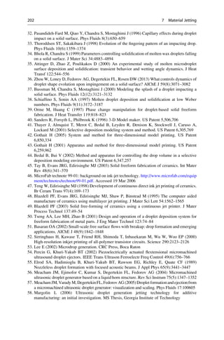

![Binder Jetting
8
Abstract
Binder jetting methods were developed in the early 1990s, primarily at MIT.
They developed what they called the 3D Printing (3DP) process in which a
binder is printed onto a powder bed to form part cross sections. This concept can
be contrasted with powder bed fusion (PBF), where a laser melts powder
particles to define a part cross section. A wide range of polymer composite,
metals, and ceramic materials have been demonstrated, but only a subset of these
are commercially available. Some binder jetting machines contain nozzles that
print color, not binder, enabling the fabrication of parts with many colors.
Several companies licensed the 3DP technology from MIT and became success-
ful machine developers, including ExOne and ZCorp (purchased by 3D Systems
in 2011). A novel continuous printing technology was been developed recently
by Voxeljet that can, in principle, fabricate parts of unlimited length.
8.1 Introduction
The original name for binder jetting was Three-Dimensional Printing (3DP) and it
was invented at MIT and has been licensed to more than five companies for
commercialization. In contrast to the printing processes described in Chap. 7,
binder jetting (BJ) processes print a binder into a powder bed to fabricate a part.
Hence, in BJ, only a small portion of the part material is delivered through the print
head. Most of the part material is comprised of powder in the powder bed.
Typically, binder droplets (80 μm in diameter) form spherical agglomerates of
binder liquid and powder particles as well as provide bonding to the previously
printed layer. Once a layer is printed, the powder bed is lowered and a new layer of
powder is spread onto it (typically via a counter-rotating rolling mechanism) [1],
very similar to the recoating methods used in powder bed fusion processes, as
presented in Chap. 5. This process (printing binder into bed; recoating bed with new
# Springer Science+Business Media New York 2015
I. Gibson et al., Additive Manufacturing Technologies,
DOI 10.1007/978-1-4939-2113-3_8
205](https://image.slidesharecdn.com/1-230308091212-68402451/85/1-Additive-manufacturing-pdf-223-320.jpg)
![layer of powder) is repeated until the part, or array of parts, is completed. A
schematic of the BJ process is shown in Fig. 8.1.
Because the printer head contains several ejection nozzles, BJ features several
parallel one-dimensional avenues for patterning. Since the process can be econom-
ically scaled by simply increasing the number of printer nozzles, the process is
considered a scalable, line-wise patterning process. Such embodiments typically
have a high deposition speed at a relatively low cost (due to the lack of a high-
powered energy source) [1], which is the case for BJ machines.
The printed part is typically left in the powder bed after its completion in order
for the binder to fully set and for the green part to gain strength. Post-processing
involves removing the part from the powder bed, removing unbound powder via
pressurized air, and infiltrating the part with an infiltrant to make it stronger and
possibly to impart other mechanical properties.
The BJ process shares many of the same advantages of powder bed processes.
Parts are self-supporting in the powder bed so that support structures are not
needed. Similar to other processes, parts can be arrayed in one layer and stacked
in the powder bed to greatly increase the number of parts that can be built at one
time. Finally, assemblies of parts and kinematic joints can be fabricated since loose
powder can be removed between the parts.
Applications of BJ processes are highly dependent upon the material being
processed. Low-cost BJ machines use a plaster-based powder and a water-based
binder to fabricate parts. Polymer powders are also available. Some machines have
color print heads and can print visually attractive parts. With this capability, a
market has developed for colorful figures from various computer games, as well as
personal busts or sculptures, with images taken from cameras. Infiltrants are used to
strengthen the parts after they are removed from the powder bed. With either
the starch or polymer powders, parts are typically considered visual prototypes or
X-Y positioning system
Part
Powder spreader
Inkjet print head
Unused powder
Build platform
Z
Binder droplets
Fig. 8.1 Schematic of the binder jetting process
206 8 Binder Jetting](https://image.slidesharecdn.com/1-230308091212-68402451/85/1-Additive-manufacturing-pdf-224-320.jpg)
![light-duty functional prototypes. In some cases, particularly with elastomeric
infiltrants, parts can be used for functional purposes. With polymer powders and
wax-based infiltrants, parts can be used as patterns for investment casting, since the
powder and wax can burn off easily.
For metal powders, parts can be used as functional prototypes or for production
purposes, provided that the parts have been designed specifically for the metal
alloys available. Molds and cores for sand casting can be fabricated by some BJ
machines that use silica or foundry sand as the powder. This is a sizable application
in the automotive and heavy equipment industries.
8.2 Materials
8.2.1 Commercially Available Materials
When Z Corporation first started in the mid-1990s, their first material was starch
based and used a water-based binder similar to a standard house-hold glue. At
present, the commercially available powder from 3D Systems is plaster based
(calcium sulfate hemihydrate) and the binder is water based [2]. Printed parts are
fairly weak, so they are typically infiltrated with another material. 3D Systems
provides three infiltrants, the ColorBond infiltrant, which is acrylate-based and is
similar to superglue, StrengthMax infiltrant which is a two-part infiltrant, and Salt
Water Cure, an eco-friendly and hazard-free infiltrant. Strength, stiffness, and
elongation data are given on 3D Systems’ web site for parts fabricated with these
infiltrants. In general, parts with any of the infiltrants are much stiffer than typical
thermoplastics or VP resins, but are less strong, and have very low elongation at
break (0.04–0.23 %).
Voxeljet [3], on the other hand, supplies a PMMA (poly-methyl methacrylate)
powder and uses a liquid binder that reacts at room temperature. They recommend
that parts stay in the powder bed for several hours to ensure that the binder is
completely cured. For investment casting pattern fabrication, they offer a
wax-based binder for use with PMMA powder that is somewhat larger in particle
size than the powder used for parts. They claim excellent pattern burnout for
investment casting.
For materials from both companies, unprinted powders are fully recyclable,
meaning that they can be reused in subsequent builds. A desirable characteristic
of powders is a high packing density so that printed parts have a high volume
fraction of powder and are strong enough to survive depowdering and clean up
operations. High packing densities can be achieved by tailoring powder particle
shape or by including a range of particle sizes so that small particles fill in gaps
between larger particles. In practice, both approaches are used whenever possible.
Quite a few other infiltrant materials have been marketed by ZCorp and 3D
Systems and many users have experimented with a variety of materials, so
alternatives are possible that can produce parts with a wide range of mechanical
properties.
8.2 Materials 207](https://image.slidesharecdn.com/1-230308091212-68402451/85/1-Additive-manufacturing-pdf-225-320.jpg)
![ExOne markets machines that use either metal or sand powders for metal parts or
sand-casting molds and cores, respectively [4]. In the metals area, they currently
market 3,166 stainless steel and bronze, 420 stainless steel (non-annealed),
420 stainless steel (annealed), bronze, and Inconel 625. For the stainless steel
materials, bronze is used as an infiltrant so that parts are virtually fully dense.
Polymer binders are used for the metals. In order to fabricate a metal part, the
“green” part is removed from the AM machine, then is subject to three furnace
cycles. In the first cycle, low temperature is used for several hours to burn off the
polymer binder. In the second cycle, high temperature is used to lightly sinter the
metal particles together so that the part has decent strength. If this cycle is too long,
the metal particles more completely melt, causing the part to lose dimensional
accuracy and its desired shape. After this cycle, the part is approximately 60 %
dense. In the final cycle, a bronze ingot is placed in the furnace in contact with the
part so that bronze infiltrates into the part’s pores, resulting in parts that are 90–
95 % dense.
An exception to the light sintering and infiltration process is the new Inconel
625 material announced by ExOne in 2014. Although they use a binder, the Inconel
material can be sintered to virtually full density (ExOne claims greater than 99 %
dense) while maintaining acceptable dimensional accuracy. If this process can be
extended to other metals, it could change the economics of metal AM significantly.
Both ExOne and Voxeljet market machines that use sand for the fabrication of
molds and cores for sand casting. ExOne offers a silica sand and two-part binder,
where one part (binder catalyst) is coated on a layer and the second part is printed
onto the layer, causing a polymerization reaction to occur and binding sand
particles together. They claim that only standard foundry materials are used so
that resulting molds and cores enable easy integration into existing manufacturing
and foundry processes. Voxeljet also offers a silica sand with an inorganic binder
and claims that their materials also integrate well into existing foundry processes.
Finally, ExOne markets a soda-lime glass material for use in fabricating artwork,
jewelry, or other decorative objects. Different colors and finishes are available. An
organic binder is used that requires an elevated temperature curing cycle. Then,
parts need to be fired at high temperature to sinter the glass particles and impart
decent strength and stiffness.
8.2.2 Ceramic Materials in Research
A wide range of materials has been developed for BJ by researchers. Printing into
metal and ceramic powder beds was first demonstrated in the early 1990s. Various
powder mixes, including compositions and size distributions, have been explored.
Traditional powder-based BJ of ceramics involves the selective printing of a
binder over a bed of ceramic powder [5]. Fabrication of ceramic parts follows a
very similar process compared with metal parts. Green parts created by this process
are subjected to a thermal decomposition prior to sintering to remove the polymer
binder. After binder burn off, the furnace temperature is increased until the
208 8 Binder Jetting](https://image.slidesharecdn.com/1-230308091212-68402451/85/1-Additive-manufacturing-pdf-226-320.jpg)
![ceramic’s sintering temperature is reached. Sometimes an infiltrant is used that
reacts to form a ceramic binder. Another possibility is to infiltrate with a metal to
form a ceramic-metal composite. The first report of using BJ for the fabrication of
ceramics was in 1993; fired components were reported as typically greater than
99.2 % dense [5]. Alumina, silica, and titanium dioxide have been made with this
process [6].
Research involving the BJ of ceramics encountered early setbacks because of the
use of dry powders. The fine powders needed for good powder bed density did not
generally flow well enough to spread into defect-free layers [5]. Furthermore, since
green part density was inadequate with the use of dry powders, isostatic pressing
was implemented after the printing process. This extraneous requirement severely
limits the types of part shapes capable of being processed.
To counteract the problems encountered with recoating a dry powder bed,
research on ceramic BJ has shifted to the use of a slurry-based working material.
In this approach, layers are first deposited by ink-jet printing a layer of slurry over
the build area. After the slurry dries, binder is selectively printed to define the part
shape. This is repeated for each individual layer, at the cost of significantly
increased build time. Multiple jets containing different material composition or
concentration could be employed to prepare components with composition and
density variation on a fine scale (100 μm) [7]. Alumina and silicon nitride have been
processed with this technique, improving green part density to 67 %, and utilizing
layer thicknesses as small as 10 μm [8].
Recently, a variation of this method was developed to fabricate metal parts
starting with metal-oxide powders [9]. The ceramic BJ is used until the furnace
sintering step. While in the furnace, a hydrogen atmosphere is introduced, causing a
reduction reaction to occur between the hydrogen and the oxygen atoms in the
metal-oxide. The reduction reaction converts the oxide to metal. After reduction,
the metal particles are sintered to form a metal part. This process has been
demonstrated for several material systems, including iron, steels, and copper.
Unfortunately, reaction thermodynamics prevent alumina and titanium oxide
from being reduced to aluminum and titanium, respectively.
This Metal-Oxide Reduction 3DP (MO3DP) process was demonstrated using a
Z405 machine [10]. Metal-oxide powders containing iron oxide, chromium oxide,
and a small amount of molybdenum were prepared by spray drying the powder
composition with polyvinyl alcohol (PVA) to form clusters of powder particles
coated with PVA. Upon reduction, the material composition formed a maraging
steel. Water was selectively printed into the powder bed to define part cross
sections, since the water will dissolve PVA, causing the clusters to stick together.
A variety of shapes (trusses, channels, thin walls) were fabricated using the process
to demonstrate the feasibility of producing cellular materials.
The main advantage of BJ, in the context of manufacturing cellular materials,
lies in its economic considerations. Simply put, the BJ process does not require high
energy, does not involve lasers or any toxic materials, and is relatively inexpensive
and fast. Part creation rate is limited to approximately twice the binder flow rate. A
typical inkjet nozzle delivers approximately 1 cm3
/min of binder; thus a machine
8.2 Materials 209](https://image.slidesharecdn.com/1-230308091212-68402451/85/1-Additive-manufacturing-pdf-227-320.jpg)
![with a 100 nozzle print head could create up to approximately 200 cm3
/min of
printed component. Because commercial inkjet printers exist with up to 1,600
nozzles, BJ could be fast enough to be used as a production process.
8.3 Process Variations
Almost all commercially available BJ machines use the architecture shown in
Fig. 8.1. An array of print heads is mounted on an XY translation mechanism. If
the process is capable of printing colored parts, some print heads are dedicated to
printing binder material, while others are dedicated to printing color. Typically, the
print heads used are standard, off-the-shelf print heads that are found in machines
for 2D printing of posters, banners, and similar applications. Parts are fabricated in
batches, just like every other AM process.
Powder handling and recoating systems are similar to those used in powder bed
fusion processes. Differences arise when comparing low-cost visual model printers
(for plaster or polymer powders) to the metal or sand printers. For the low-cost
printers, powder containers (vats) can be hand-carried. In the latter cases, however,
powder beds can weigh hundreds or thousands of pounds, necessitating different
material handling and powder bed manipulation methods. For the sand printers, the
vats utilize a rail system for conveying powder beds to and from depowdering
stations and cranes are used for transporting parts or molds.
The capability of continuous printing or of fabricating parts that are larger than
the AM machine fabricating them has been discussed in the research community. In
recent years, two different approaches have been demonstrated for continuous
printing of parts. One approach is being commercialized by Voxeljet in 2013 and
is based on linear translation of the part being fabricated. The second approach is
called spiral growth manufacturing and was developed by researchers at the
University of Liverpool, UK.
The Voxeljet continuous printing process is a novel idea that utilizes an inclined
build plane. That is, the build surface of the powder bed is inclined at an angle of
30
, less than the powder’s critical angle of repose. Powder recoating and binder
jetting are performed on this inclined build surface. The powder bed translates on a
conveyor belt from the front towards the back of the machine. In contrast to typical
batch fabrication, parts emerge continuously at the back of the machine. In princi-
ple, parts could be infinitely long, certainly much longer than the machine. The
continuous part fabrication capability could represent an important step in achiev-
ing economical manufacture of moderate to high production volumes of parts.
The second continuous fabrication approach, spiral growth manufacturing
(SGM) was invented by Chris Sutcliffe at the University of Liverpool in the early
2000s. The patent US2008109102 is a good reference for further information
[11]. In the BJ variant of SGM, the powder bed is circular and rotates continuously.
Binder printing and recoating are performed continuously also. As the machine
operates, the powder bed indexes downwards continuously to accommodate the
210 8 Binder Jetting](https://image.slidesharecdn.com/1-230308091212-68402451/85/1-Additive-manufacturing-pdf-228-320.jpg)
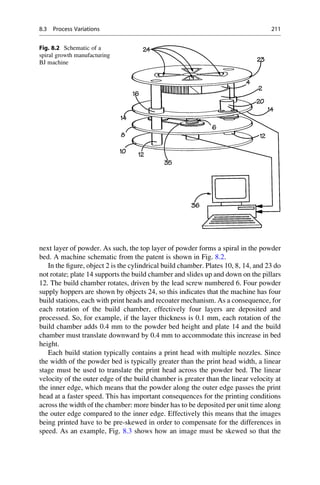
![printed image is fabricated properly [12]. This image was printed on a SGM
machine with two print heads, hence the two images on the right. Note that the
inner edge is on the left side of the image, which is stretched, while the outer edge is
compressed.
8.4 BJ Machines
A wide variety of powder and binder materials can be used which enables signifi-
cant flexibility in the process. MIT licensed the BJ technology according to the type
of material and application that each licensee was allowed to exploit. ZCorp, Inc.
was one company that marketed machines that build concept models in starch and
plaster powder using a low viscosity glue as binder. At the other end of the
spectrum, ExOne markets machines that build in metal powder, with a strong
polymer material that is used as the binder, as well as silica sand for sand casting
applications. Voxeljet is a relatively new company that markets BJ machines that
use polymer and sand powders for concept models, functional models, investment
casting patterns, and sand casting applications.
As of 2012, ZCorp was purchased by 3D Systems and their product line was
merged into 3D Systems’ ProJet line of printers. These printers are now branded as
the ProJet X60 line of printers, with the smallest being the ProJet 160 and the largest
being the ProJet 860Pro. Specifications for some of these machines are shown in
Table 8.1. Machine names consisting only of numbers fabricate parts that are
monochrome only, while suffixes of C, Plus, or Pro indicate that parts can be
printed in color, up to the full CMYK color model (Cyan, Magenta, Yellow, Key
(black)).
Voxeljet sold their first machine in 2005. They now offer a range of machines
from the smallest VX200 to the huge VX4000, which has a 4 m long powder bed.
The VX4000 processes foundry sand materials for the sand casting industry. They
also market the VXC800, which is the infinitely continuous printer that was
Fig. 8.3 Skewing an image for SGM printing
212 8 Binder Jetting](https://image.slidesharecdn.com/1-230308091212-68402451/85/1-Additive-manufacturing-pdf-230-320.jpg)

![described earlier. A photo of the VXC800 is shown in Fig. 8.4. For this machine, the
layer thickness is 150–400 μm and they use 600 dpi print heads. The surface area of
the inclined plane is 500 850 mm.
The ExOne Corporation markets a line of BJ machines that fabricate metal parts
and sand casting molds and cores in foundry sand. Strong polymer binders are
required with these heavy powders. As explained earlier, nearly fully dense parts
can be fabricated by printing binder into the metal bed, burning off the binder in a
furnace at a low temperature, sintering the metal powder during a high temperature
furnace cycle, then infiltrating a second metal, such as copper or bronze, at a low
temperature. The printed part, when removed from the bed, is a relatively
low-density (50–60 %) green part. Other than how the green part is formed, this
process is identical to the indirect processing approach for metal and ceramic part
fabrication discussed in Chap. 5 and illustrated in Fig. 5.7. Stainless steel-bronze
parts have been made with this technology [4]. The process is typically accurate to
0.125 mm. Several ExOne machine models are also listed in Table 8.1.
Applications for the metal material models include prototypes of metal parts and
some low-volume manufacturing, as well as tooling. As parts are fabricated in a
powder bed, the surface finish of these parts is comparable to PBF parts. Finish
machining is thus required for high tolerance and mating surfaces. ExOne markets
another machine that fabricates gold dental restorations, for example, copings for
crowns. The materials and binder printing system were developed specifically for
this application, since higher resolution is needed.
In the tooling area, ExOne promotes the advantages of conformal cooling in
injection molds. In conformal cooling, cooling channels are routed close to the
surfaces of the part cavity, particularly where hot spots are predicted. Using
conventional machining processes, cooling channels are drilled as straight holes.
With AM processes, however, cooling channels of virtually any shape and configu-
ration can be designed into tools. Figure 8.5 illustrates one tool design with
conformal cooling channels that was fabricated in an ExOne machine.
Fig. 8.4 Voxeljet VXC800
machine (Courtesy Voxeljet)
214 8 Binder Jetting](https://image.slidesharecdn.com/1-230308091212-68402451/85/1-Additive-manufacturing-pdf-232-320.jpg)
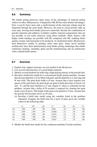
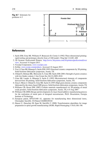

![the substrate and is then formed into the cross-sectional shape (“bond-then-form”
processes). For other processes the laminate is first cut and then bonded to the
substrate (“form-then-bond” processes).
9.1.2 Bond-Then-Form Processes
In “bond-then-form” processes, the building process typically consists of three
steps in the following sequence: placing the laminate, bonding it to the substrate,
and cutting it according to the slice contour. The original LOM machines used this
process with adhesive-backed rolls of material. A heated roller passes across the
sheet after placing it for each layer, melting the adhesive and producing a bond
between layers. A laser (or in some cases a mechanical cutting knife) designed to
cut to a depth of one layer thickness cuts the cross-sectional outline based on the
slice information. The unused material is left in place as support material and is
diced using a crosshatch pattern into small rectangular pieces called “tiles” or
“cubes.” This process of bonding and cutting is repeated until the complete part
is built. After part construction, the part block is taken out and post-processed. The
crosshatched pieces of excess material are separated from the part using typical
wood carving tools (called decubing). It is relatively difficult to remove the part
from the part block when it is cold, therefore, it is often put into an oven for some
time before decubing or the part block is processed immediately after part buildup.
Although historically many people continue to associate paper sheet lamination
with the LOM machines introduced in 1991 by Helisys Inc., USA and subsequently
supported by Cubic Technologies, USA (after Helisys’ bankruptcy), new paper-
based sheet lamination machines are currently sold by Mcor Technologies (Ireland)
Fig. 9.1 Schematic of the LOM process (based on [1] Journal of Materials Processing Technol-
ogy by D.I. Wimpenny, B. Bryden, I.R. Pashby. Copyright 2003 by Elsevier Science Technol-
ogy Journals. Reproduced with permission of Elsevier Science Technology Journals in the
format Textbook via Copyright Clearance Center.)
220 9 Sheet Lamination Processes](https://image.slidesharecdn.com/1-230308091212-68402451/85/1-Additive-manufacturing-pdf-238-320.jpg)
![and Wuhan Binhu (China). These new systems make use of plain paper as the build
material, and selectively dispense adhesive only where needed. Because the support
material is not adhesively bonded, unlike in LOM, the support removal process is
easier. The use of color inkjet printing onto paper by Mcor Technologies enables
the production of full-color paper parts directly from a CAD file.
Solidimension (Be’erot, Israel) took the concepts of LOM and further developed
them in 1999 into a commercial prototyping system for laminating polyvinyl
chloride (PVC) plastic sheets. Solidimension sold its own machines under the
Solido name [2] and under other names via resellers. This machine utilized an x–
y plotter for cutting the PVC sheets and for writing with “anti glue” pens, which
inhibit bonding in prescribed locations. This machine used a unique approach to
support material removal. Support material was subdivided into regions, and unique
patterns for cutting and bonding the excess material were used to enable easy
support material removal. An example of this support material strategy can be
seen in Fig. 9.2. Solido machines are no longer offered for sale, however if history is
any guide, others may pick up this unique idea and offer similar machines someday.
Bond-then-form sheet lamination principles have also been successfully applied
to fabrication of parts from metal, ceramic, and composite materials. In this case,
rather than paper or polymer sheets, ceramic or metal-filled tapes are used as the
build material to form green parts, and high-temperature furnace post-processing is
used to debind and sinter the structure. These tapes are then used for part construc-
tion employing a standard sheet lamination process.
Specific advantages of LOM-like bond-then-form adhesive-based processes
include: (a) little shrinkage, residual stresses, and distortion problems within the
process; (b) when using paper feedstock, the end material is similar to plywood, a
typical pattern making material amenable to common finishing operations; (c) large
parts can be fabricated rapidly; (d) a variety of build materials can be used,
including paper and polymer sheets and metal- or ceramic-filled tapes;
(e) nontoxic, stable, and easy-to-handle feedstock; and (f) low material, machine,
and process costs relative to other AM systems.
Fig. 9.2 Support material removal for three golf balls made using a Solidimension machine,
showing: (a) the balls still encased in a central region, being separated from the larger block of
bonded material; (b) the support material is glued in an accordion-like manner so that the excess
material can be pulled out easily as a continuous piece; and (c) the balls after complete removal of
excess support material (Courtesy 3D Systems)
9.1 Introduction 221](https://image.slidesharecdn.com/1-230308091212-68402451/85/1-Additive-manufacturing-pdf-239-320.jpg)
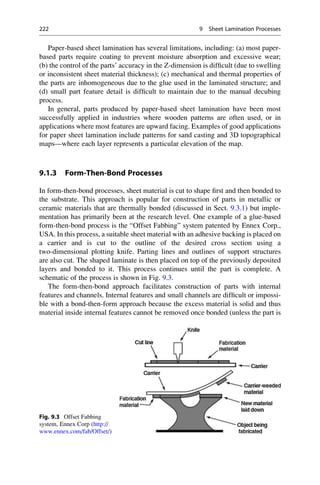
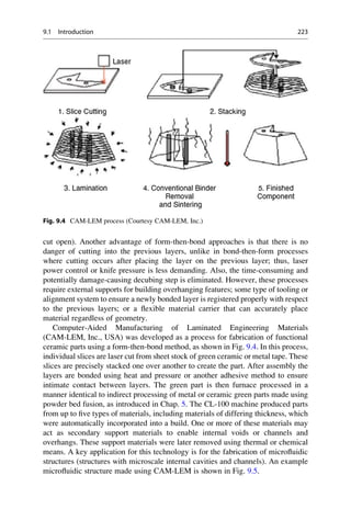
![Another example of a form then bond process is the Stratoconception approach
[3], where the model is sliced into thicker layers. These layers are machined and
then glued together to form a part. The use of a multiaxis machining center enables
the edges of each layer to be contoured to better match the STL file, helping
eliminate the stair-step effect that occurs with increasing layer thickness. This
and similar cutting techniques have been used by many different researchers to
build large structures from foam, wood, and other materials to form statues, large
works of art, and other structures.
9.2 Materials
As covered in the previous section, a wide variety of materials has been processed
using a variety of sheet lamination processes, including plastics, metals, ceramics,
and paper. A brief survey will be offered identifying the materials and their
characteristics that facilitate sheet lamination.
Butcher paper was the first material used in the original Helisys LOM process.
Butcher paper is coated on one side with a thin layer of a thermoplastic polymer. It
is this polymer coating that melts and ensures that one layer of paper bonds to the
previous layer. Since butcher paper is fairly strong and heavy, it forms sturdy parts
after a suitable thickness has been fabricated (5–6 mm typically). After part
fabrication, parts are finished as if they were wood by sanding, filing, staining,
and varnishing or sealing.
The recently developed Mcor Technologies printers use standard copy paper in
A4 or US letter sizes with weights of 20 or 43 lb. Either white or colored paper can
be used. The water-based glue binds paper sheets and results in fairly rigid parts
although, similar to the Helisys process, a minimum thickness of 5 or 6 mm is
required to ensure good strength.
Fig. 9.5 A ceramic microfluidic distillation device cutaway view (left) and finished part (right)
(Courtesy CAM-LEM, Inc.)
224 9 Sheet Lamination Processes](https://image.slidesharecdn.com/1-230308091212-68402451/85/1-Additive-manufacturing-pdf-242-320.jpg)
![9.3.1 Thermal Bonding
Many organizations around the world have successfully applied thermal bonding to
sheet lamination of functional metal parts and tooling. A few examples will be
mentioned to demonstrate the flexibility of this approach. Yi et al. [4] have
successfully fabricated 3D metallic parts using precut 1-mm thick steel sheets
that are then diffusion bonded. They demonstrated continuity in grain structure
across sheet interfaces without any physical discontinuities. Himmer et al. [5]
produced aluminum injection molding dies with intricate cooling channels using
Al 3003 sheets coated with 0.1-mm thick low-melting point Al 4343 (total sheet
thickness 2.5 mm). The sheets were laser cut to an approximate, oversized cross
section, assembled using mechanical fasteners, bonded together by heating the
assembly in a nitrogen atmosphere just above the melting point of the Al 4343
coating material, and then finish machined to the prescribed part dimensions and
surface finish. Himmer et al. [6] also demonstrated satisfactory layer bonding using
brazing and laser spot welding processes. Obikawa [7] manufactured metal parts
employing a similar process from thinner steel sheets (0.2 mm thick), with their top
and bottom surface coated with a low-melting-point alloy. Wimpenny et al. [1]
produced laminated steel tooling with conformal cooling channels by brazing laser-
cut steel sheets. Similarly, Yamasaki [8] manufactured dies for automobile body
manufacturing using 0.5-mm thick steel sheets. Each of these, and other
investigators, have shown that thermally bonding metal sheets is an effective
method for forming complex metal parts and tools, particularly those which have
internal cavities and/or cooling channels.
Although extensively studied, sheet metal lamination approaches have gained
little traction commercially. This is primarily due to the fact that bond-then-form
processes require extensive post-processing to remove support materials, and form-
then-bond processes are difficult to automate for arbitrary, complex geometries. In
the case of form-then-bond processes, particularly if a cross section has geometry
that is disconnected from the remaining geometry, accurate registration of
laminates is difficult to achieve and may require a part-specific solution. Thus,
upward-facing features where each cross section’s geometry is contiguously
interconnected are the easiest to handle. Commercial interest in sheet lamination
is primarily in the area of inexpensive, full-color paper parts and large tooling,
where internal, conformal cooling channels can provide significant benefits over
traditional cooling strategies.
Another process that combined sheet lamination with other forms of AM
(including beam deposition, extrusion, and subtractive machining) was Shape
Deposition Manufacturing (SDM) [9]. With SDM, the geometry of the part is
subdivided into nonplanar segments. Each segment is deposited as an over-sized,
near-net shape region and then finish machined. Sequential deposition and machin-
ing of segments (rather than planar layers) forms the part. A decision is made
concerning how each segment should be manufactured dependent on such factors as
the accuracy, material, geometrical features, and functional requirements. Second-
ary support materials were commonly used to enable complex geometry to be made
226 9 Sheet Lamination Processes](https://image.slidesharecdn.com/1-230308091212-68402451/85/1-Additive-manufacturing-pdf-244-320.jpg)
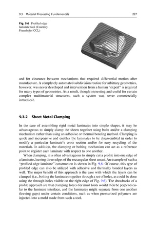
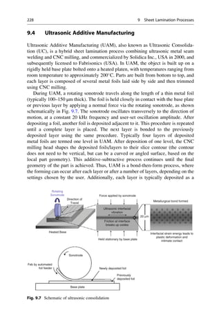
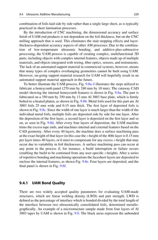
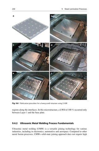
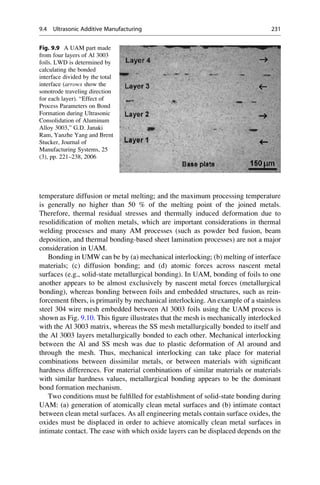
![ratio of metal-oxide hardness to base metal hardness, where higher ratios facilitate
easier removal. Due to the significant hardness differences between aluminum and
aluminum oxide, Al 3003 alloys are one of the best-suited materials for ultrasonic
welding. Nonstructural noble metals, such as gold which do not have surface oxide
layers, are quite amenable to ultrasonic welding. Materials with difficult-to-remove
oxide layers are problematic for ultrasonic welding. However, difficult-to-weld
materials have been shown to be UAM compatible when employing chemical or
mechanical techniques for removing the surface oxide layers just prior to welding.
Plastic deformation at the foil interfaces is critical for UAM, to break up surface
oxides and overcome surface roughness. The magnitude of plastic deformation
necessary to achieve bonding can be reduced by decreasing the surface roughness
of the interface materials prior to welding, such as by surface machining (which
occurred between Layer 1 and the base plate in Fig. 9.9) and/or by removing the
surface oxides by chemical stripping or surface finishing. In addition, factors which
enhance plastic deformation are also beneficial for bonding, such as using more
ductile materials and/or by thermally or acoustically softening the materials during
bonding.
Metallic materials experience property changes when subjected to ultrasonic
excitations, including acoustic softening, increase in crystallographic defects, and
enhanced diffusivities. In particular, metal softening in the presence of ultrasonic
excitations, known as the “Blaha effect” or “acoustic softening,” means that the
magnitude of stresses necessary to initiate plastic deformation are significantly
lower [10]. The softening effect of ultrasonic energy on metals is similar to the
effect of heating, and can in fact reduce the flow stress of a metallic material more
Fig. 9.10 SEM microstructures of Al 3003/SS mesh: (a) SS mesh embedded between Al 3003
layers, (b) Al 3003/SS mesh interface at a higher magnification. The white arrows illustrate the
lack of metallurgical bonding between the Al and SS materials. The black arrows indicate areas of
metallurgical bonding between SS mesh elements. # Emerald Group Publishing Limited, “Use of
Ultrasonic Consolidation for Fabrication of Multi-Material Structures,” G.D. Janaki Ram, Chris
Robinson, Yanzhe Yang and Brent Stucker, Rapid Prototyping Journal, 13 (4), pp. 226–235, 2007
232 9 Sheet Lamination Processes](https://image.slidesharecdn.com/1-230308091212-68402451/85/1-Additive-manufacturing-pdf-250-320.jpg)
![9.4.4.2 UAM Microstructures
Typical microstructures from Al 3003 tapes with representative defects were shown
in Figs. 9.9 and 9.12. Figure 9.14 shows the microstructure of two Ni 201 foils
deposited on an Al 3003 substrate. Plastic deformation of Ni foils near the foil
surfaces can be experimentally visualized using orientation imaging microscopy, as
shown in Fig. 9.15. Smooth intragrain color transition within a few grains at the
surface indicates the foil interfaces undergo some plastic deformation during UAM
processing, whereas the absence of intragranular color transitions away from the
foil surfaces indicates that the original microstructure is retained in the bulk of the
foil.
In addition to UAM of similar materials, UAM of dissimilar materials is quite
effective. Many dissimilar metal foils can be bonded with distinct interfaces, with a
high degree of LWD and without intermetallic formation [11].
Fig. 9.13 Schematic illustrating (a) 50 % foil overlap and (b) random foil overlap in UAM
Fig. 9.14 Ultrasonically consolidated Ni 201 foils
9.4 Ultrasonic Additive Manufacturing 237](https://image.slidesharecdn.com/1-230308091212-68402451/85/1-Additive-manufacturing-pdf-255-320.jpg)
![9.4.5 UAM Applications
UAM provides unique opportunities for manufacture of structures with complex
internal geometries, manufacture of structures from multiple materials, fiber
embedment during manufacture, and embedding of electronics and other features
to form smart structures. Each of these application areas is discussed below.
9.4.5.1 Internal Features
As with other AM techniques, UAM is capable of producing complex internal
features within metallic materials. These include honeycomb structures, internal
pipes or channels, and enclosed cavities. During UAM, internal geometrical
features of a part are fabricated via CNC trimming before depositing the next
layer (see Fig. 9.8). Not all internal feature types are possible, and all of the “top”
surface of internal features will have a stair-step geometry and not a CNC-milled
surface, as the CNC can only mill the upward-facing surfaces of internal
geometries. After fabrication of an internal feature is completed, metal foils are
placed over the cavities or channels and welded, thus enclosing the internal
features.
It has been shown that it becomes quite difficult to bond parts using UAM when
their height-to-width ratio is near 1:1 [12]. In order to achieve higher ratios, support
materials or other restraints are necessary to make the part rigid enough such that
there is differential motion between the existing part and the foils that are being
added. The development of an effective support material dispensing system for
UAM would dramatically increase its ability to make more free-form shapes and
larger internal features. Without support materials, internal features must be
designed and oriented in such a way that the sonotrode is always supported by an
existing, rigid feature while depositing a subsequent layer. As a result, for instance,
internal cooling channels cannot be perpendicular to the sonotrode traveling direc-
tion, and honeycomb structures must be small enough that there are always at least
two ribs supporting the deposition of the foil face sheets.
9.4.5.2 Material Flexibility
A wide range of metallic materials has been used with UAM. Theoretically, any
metal which can be ultrasonically welded is a candidate material for the UAM
process. Materials which have been successfully bonded using UAM include Al
3003 (H18 and O condition), Al 6061, Al 2024, Inconel®
600, brass, SS 316, SS
347, Ni 201, and high purity copper. Ultrasonic weldabilities of a number of other
metallic materials have been widely demonstrated [11, 13–16]. Thus, there is
significant material flexibility for UAM processes. In addition to metal foils,
other materials have been used, including MetPreg®
(an alumina fiber-reinforced
Al matrix composite tape) and prewoven stainless steel AISI 304 wire meshes (see
Fig. 9.10), which both have been bonded to Al 3003 using UAM.
By depositing various metal foils at different desired layers or locations during
UAM, multimaterial structures or functionally gradient materials can be produced.
Composition variation and resultant property changes can be designed to meet
9.4 Ultrasonic Additive Manufacturing 239](https://image.slidesharecdn.com/1-230308091212-68402451/85/1-Additive-manufacturing-pdf-257-320.jpg)
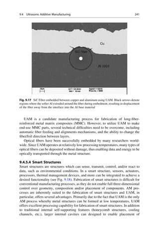
![electronics, actuators, heat pipes, or other features at optimum location within a
structure [17]. Many types of embedded electronics, sensors, and thermal manage-
ment devices have been inserted into UAM cavities. Sensors for recording temper-
ature, acceleration, stress, strain, magnetism, and other environmental factors have
been fully encapsulated and have remained functional after UAM embedment. In
addition to prefabricated electronics, it is feasible to fabricate customized electron-
ics in UAM with the integration of direct write technologies (see Chap. 11). By
combining UAM with direct write, electronic features (conductors, insulators,
batteries, capacitors, etc.) can be directly created within or on UAM-made
structures in an automated manner.
9.5 Conclusions
As illustrated in this chapter, a broad range of sheet lamination techniques exist.
From the initial LOM paper-based technology to the more recent UAM approach,
sheet lamination processes have shown themselves to be robust, flexible, and
valuable for many applications and materials. The basic method of trimming a
sheet of material to form a cross-sectional layer is inherently fast, as trimming only
occurs at the layer’s outline rather than needing to melt or cure the entire cross-
sectional area to form a layer. This means that sheet lamination approaches exhibit
the speed benefits of a layer-wise process while still utilizing a point-wise energy
source. Many variations of sheet lamination processes have been demonstrated,
which have proved to be suitable for many different types of metal, ceramic,
polymer, and paper materials.
Computational
Device
Patch
antenna
Thermocouple
Encapsulated components via AM technology
Wiring
Solar Panel
Sensor and Integrated
Electronics
Fig. 9.18 Schematic illustrating the creation of a smart structure using UAM
242 9 Sheet Lamination Processes](https://image.slidesharecdn.com/1-230308091212-68402451/85/1-Additive-manufacturing-pdf-260-320.jpg)

![Directed Energy Deposition Processes
10
10.1 Introduction
Directed energy deposition (DED) processes enable the creation of parts by melting
material as it is being deposited. Although this basic approach can work for
polymers, ceramics, and metal matrix composites, it is predominantly used for
metal powders. Thus, this technology is often referred to as “metal deposition”
technology.
DED processes direct energy into a narrow, focused region to heat a substrate,
melting the substrate and simultaneously melting material that is being deposited
into the substrate’s melt pool. Unlike powder bed fusion techniques (see Chap. 5)
DED processes are NOT used to melt a material that is pre-laid in a powder bed but
are used to melt materials as they are being deposited.
DED processes use a focused heat source (typically a laser or electron beam) to
melt the feedstock material and build up three-dimensional objects in a manner
similar to the extrusion-based processes from Chap. 6. Each pass of the DED head
creates a track of solidified material, and adjacent lines of material make up layers.
Complex three-dimensional geometry requires either support material or a
multiaxis deposition head. A schematic representation of a DED process using
powder feedstock material and laser is shown in Fig. 10.1.
Commercial DED processes include using a laser or electron beam to melt
powders or wires. In many ways, DED techniques can be used in an identical
manner to laser cladding and plasma welding machines. For the purposes of this
chapter, however, DED machines are considered those which are designed to create
complex 3D shapes directly from CAD files, rather than the traditional welding and
cladding technologies, which were designed for repair, joining, or to apply coatings
and do not typically use 3D CAD data as an input format.
A number of organizations have developed DED machines using lasers and
powder feeders. These machines have been referred to as Laser Engineered Net
Shaping (LENS) [1], Directed Light Fabrication (DLF) [2], Direct Metal Deposi-
tion (DMD), 3D Laser Cladding, Laser Generation, Laser-Based Metal Deposition
# Springer Science+Business Media New York 2015
I. Gibson et al., Additive Manufacturing Technologies,
DOI 10.1007/978-1-4939-2113-3_10
245](https://image.slidesharecdn.com/1-230308091212-68402451/85/1-Additive-manufacturing-pdf-263-320.jpg)
![(LBMD), Laser Freeform Fabrication (LFF), Laser Direct Casting, LaserCast [3],
Laser Consolidation, LasForm, and others. Although the general approach is the
same, differences between these machines commonly include changes in laser
power, laser spot size, laser type, powder delivery method, inert gas delivery
method, feedback control scheme, and/or the type of motion control utilized.
Because these processes all involve deposition, melting and solidification of pow-
dered material using a traveling melt pool, the resulting parts attain a high density
during the build process. The microstructure of parts made from DED processes
(Figs. 10.2 and 10.3) are similar to powder bed fusion processes (see Fig. 5.14),
wherein each pass of the laser or heat source creates a track of rapidly solidified
material.
As can be seen from Figs. 10.2 and 10.3, the microstructure of a DED part can be
different between layers and even within layers. In the Ti/TiC deposit shown in
Fig. 10.2, the larger particles present in the microstructure are unmelted carbides.
The presence of fewer unmelted carbides in a particular region is due to a higher
overall heat input for that region of the melt pool. By changing process parameters,
it is possible to create fewer or more unmelted carbides within a layer, and by
increasing laser power, for instance, a greater amount of the previously deposited
layer (or substrate for the first layer) will be remelted. By comparing the thickness
of the last-deposited layer with the first- or second-deposited layer (such as in
Fig. 10.3a), an estimate of the proportion of a layer that is remelted during
subsequent deposition can be made. Each of these issues is discussed in the
following section.
Laser beam
Powder Feed
Nozzles
Powder stream
Layer thickness
Track width
Motion
Fig. 10.1 Schematic of a
typical laser powder DED
process
246 10 Directed Energy Deposition Processes](https://image.slidesharecdn.com/1-230308091212-68402451/85/1-Additive-manufacturing-pdf-264-320.jpg)
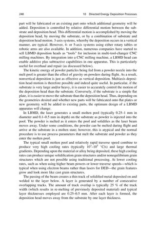
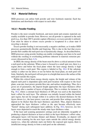
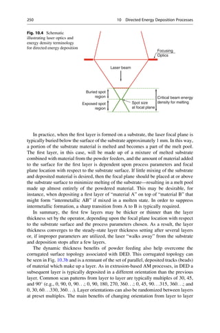
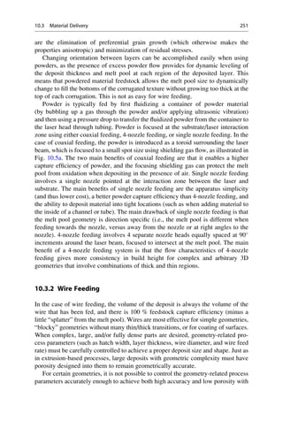
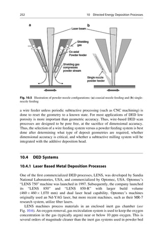
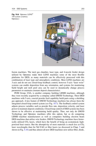
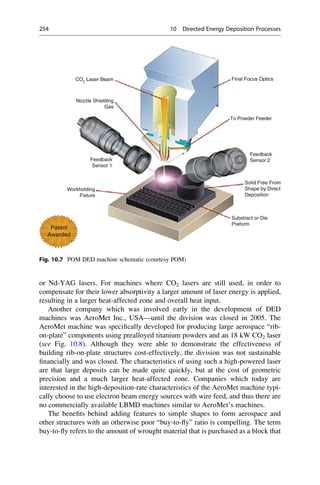
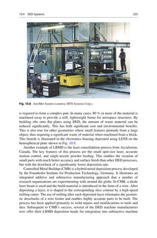
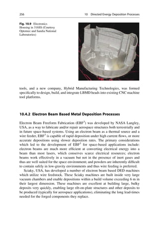
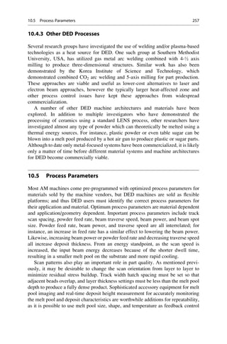

![diffusion controlled solid-state phase transformations; (b) formation of supersatu-
rated solutions and nonequilibrium phases; (c) formation of extremely fine
microstructures with dramatically reduced elemental segregation; and
(d) formation of very fine secondary phase particles (inclusions, carbides, etc.).
Parts produced using DED experience a complex thermal history in a manner very
similar to multi-pass weld deposits. Changes in cooling rate during part construc-
tion can occur due to heat buildup, especially in thin-wall sections. Also, energy
introduced during deposition of subsequent layers can reheat previously deposited
material, changing the microstructure of previously deposited layers. The thermal
history, including peak temperatures, time at peak temperature, and cooling rates,
can be different at each point in a part, leading to phase transformations and a
variety of microstructures within a single component.
As shown in Figs. 10.2, 10.3, and 10.10, parts made using DED typically exhibit
a layered microstructure with an extremely fine solidification substructure. The
interface region generally shows no visible porosity and a thin heat-affected zone
Fig. 10.10 Smooth
transition between a 100 %
Ti-6-4 and 100 % Ti-22-23
alloy in the gage section of a
tensile bar. The transition
region is shown at higher
magnification (courtesy
Optomec)
−0.3
138
140
142
144
146
148
150
152
−0.2 −0.1 0
X [In]
σ
0
2%
[ksi]
0.1 0.2 0.3
Fig. 10.11 Yield strength at various locations along the tensile bar from Fig. 10.10 representing
the mechanical properties for different combinations of Ti-6-4 and Ti-22-23 (courtesy Optomec)
10.6 Typical Materials and Microstructure 259](https://image.slidesharecdn.com/1-230308091212-68402451/85/1-Additive-manufacturing-pdf-277-320.jpg)
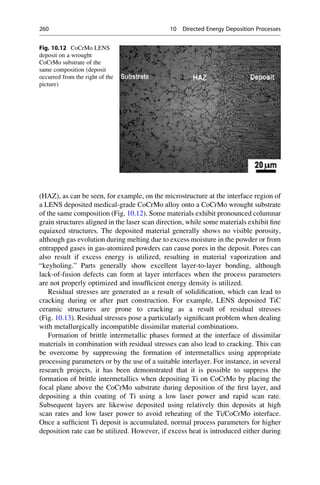
![the deposition of subsequent layers or in subsequent heat treatment, equilibrium
intermetallics will form and cracking and delamination occurs. In other work,
CoCrMo has been successfully deposited on a porous Ta substrate when employing
Zr as an interlayer material, a combination that is otherwise prone to cracking and
delamination.
It is common for laser deposited parts to exhibit superior yield and tensile
strengths because of their fine grain structure. Ductility of DED parts, however, is
generally considered to be inferior to wrought or cast equivalents. Layer orientation
can have a great influence on % elongation, with the worst being the z direction.
However, in many alloys ductility can be recovered and anisotropy minimized by
heat treatment—without significant loss of strength in most cases.
10.7 Processing–Structure–Properties Relationships
Parts produced in DED processes exhibit high cooling rate cast microstructures.
Processing conditions influence the solidification microstructure in ways that can be
predicted in part by rapid solidification theory. For a specific material, solidification
microstructure depends on the local solidification conditions, specifically the solid-
ification rate and temperature gradient at the solid/liquid interface. By calculating
the solidification rate and thermal gradient, the microstructure can be predicted
based upon calibrated “solidification maps” from the literature.
To better understand solidification microstructures in DED processes, Beuth and
Klingbeil [5] have developed procedures for calculating thermal gradients, G,
and solidification rates, R, analytically and numerically. These calculated G and
R values can then be plotted on solidification maps to determine the types of
microstructures which can be achieved with different DED equipment, process
parameters, and material combinations. Solutions for both thin walls [5] and bulky
deposits [6] have been described. For brevity’s sake, the latter work by Bontha
Fig. 10.13 Cracks in a TiC
LENS deposit due to residual
stresses [4] (SCRIPTA
MATERIALIA by Weiping
Liu, and J. N. DuPont.
Copyright 2003 by Elsevier
Science Technology
Journals. Reproduced with
permission of Elsevier
Science Technology
Journals in the format
Textbook via Copyright
Clearance Center)
10.7 Processing–Structure–Properties Relationships 261](https://image.slidesharecdn.com/1-230308091212-68402451/85/1-Additive-manufacturing-pdf-279-320.jpg)
![et al. [6] based upon the 3D Rosenthal solution for a moving point heat source on an
infinite substrate will be introduced here (Fig. 10.14). This 3D Rosenthal solution
also has been applied to PBF techniques in an identical fashion.
In this simplified model, material deposition is ignored. The model considers
only heat conduction within the melt pool and substrate due to a traveling heat
source moving at velocity, V. The fraction of impinging energy absorbed is αQ,
which is a simplification of the physically complex temperature-dependent absorp-
tion of the beam by regions of the melt pool and solid, absorption of energy by
powder in flight, and other factors. Thus a single parameter, α, represents the
fraction of impinging beam energy power absorbed.
It is assumed the beam moves only in the x direction, and thus the beam’s
relative coordinates (x0, y0, z0) from Fig. 10.14 are related to the fixed coordinates
(x, y, z) at any time t as (x0, y0, z0) ¼ (x Vt, y, z).
With the above conditions, the Rosenthal solution for temperature T at time t for
any location in an infinite half-space can be expressed in dimensionless form as:
T ¼
e x0þ
ffiffiffiffiffiffiffiffiffiffiffiffiffiffi
x2
0þy2
0þz2
0
p
2
ffiffiffiffiffiffiffiffiffiffiffiffiffiffiffiffiffiffiffiffiffiffiffiffi
x2
0 þ y2
0 þ z2
0
q ð10:1Þ
where
T ¼
T T0
αQ=πk
ð Þ ρcV=2k
ð Þ
,
x0 ¼
x0
2k=ρcV
ð Þ
y0 ¼
y0
2k=ρcV
ð Þ
and z0 ¼
z0
2k=ρcV
ð Þ
:
ð10:2Þ
In these equations, T0 is the initial temperature, and ρ, c, and k are density, specific
heat, and thermal conductivity of the substrate, respectively. In this simplified
model, the thermophysical properties are assumed to be temperature independent,
Fig. 10.14 3D Rosenthal
geometry considered
262 10 Directed Energy Deposition Processes](https://image.slidesharecdn.com/1-230308091212-68402451/85/1-Additive-manufacturing-pdf-280-320.jpg)
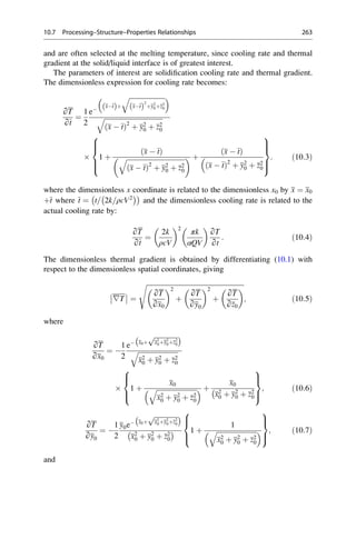
![∂T
∂z0
¼
1
2
z0e x0þ
ffiffiffiffiffiffiffiffiffiffiffiffiffiffi
x2
0þy2
0þz2
0
p
x2
0 þ y2
0 þ z2
0
1 þ
1
ffiffiffiffiffiffiffiffiffiffiffiffiffiffiffiffiffiffiffiffiffiffiffiffi
x2
0 þ y2
0 þ z2
0
q
8
:
9
=
;
: ð10:8Þ
As defined above, the relationship between the dimensionless thermal gradient
∇T and the actual thermal gradient |∇T| is given by
∇T ¼
2k
ρcV
2
πk
αQ
∇T
j j: ð10:9Þ
Using this formulation, temperature, cooling rates, and thermal gradients can be
solved for any location (x, y, z) and time (t).
For microstructure prediction purposes, solidification characteristics are of
interest; and thus we need to know the cooling rate and thermal gradients at the
boundary of the melt pool. The roots of (10.1) can be solved numerically for
temperature T equal to melting temperature Tm to find the dimensions of the melt
pool. Similarly to (10.2) for normalized temperature, normalized melting tempera-
ture can be represented by:
Tm ¼
Tm T0
αQ=πk
ð Þ ρcV=2k
ð Þ
: ð10:10Þ
Given cooling rate ∂T
∂t
from (10.4) and thermal gradient, G, defined as G ¼ |∇T|, we
can define the solidification velocity, R, as
R ¼
1
G
∂T
∂t
: ð10:11Þ
We can now solve these sets of equations for specific process parameters (i.e., laser
power, velocity, and material properties) for a machine/material combination of
interest. After this derivation, Bontha et al. [6] used this analytical model to
demonstrate the difference between solidification microstructures which can be
achieved using a small scale DED process with a lower-powered laser beam, such
as utilized in a LENS machine, compared to a high-powered laser beam system,
such as practiced by AeroMet for Ti–6Al–4 V. Assumptions included the
thermophysical properties of Ti–6Al–4 V at Tm ¼ 1,654
C, a room temperature
initial substrate temperature T0 ¼ 25
C, fraction of energy absorbed α ¼ 35, laser
power from 350 to 850 W, and beam velocity ranging from 2.12 to 10.6 mm/s. For
the high-powered beam system, a laser power range from 5 to 30 kW was selected.
A set of graphs representing microstructures with low-powered systems is shown in
Fig. 10.15. Microstructures from high-powered systems are shown in Fig. 10.16 for
comparison.
As can be seen from Fig. 10.15, lower-powered DED systems cannot create
mixed or equiaxed Ti–6Al–4 V microstructures, as the lower overall heat input
264 10 Directed Energy Deposition Processes](https://image.slidesharecdn.com/1-230308091212-68402451/85/1-Additive-manufacturing-pdf-282-320.jpg)
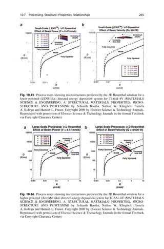
![means that there are very large thermal gradients. For higher-powered DED
systems (relevant to AeroMet-like processes and most electron beam DED pro-
cess), it is possible to create dendritic, mixed or fully equiaxed microstructures
depending upon the process parameter combinations used. As a result, without the
need for extensive experimentation, process maps such as these, when combined
with appropriate modeling, can be used to predict the type of DED system (specifi-
cally the scan rates and laser power) needed to achieve a desired microstructure
type for a particular alloy.
10.8 DED Benefits and Drawbacks
DED processes are capable of producing fully dense parts with highly controllable
microstructural features. These processes can produce functionally graded
components with composition variations in the X, Y, and Z directions.
The main limitations of DED processes are poor resolution and surface finish.
An accuracy better than 0.25 mm and a surface roughness of less than 25 μm
(arithmetic average) are difficult with most DED processes. Slower build speed is
another limitation. Build times can be very long for these processes, with typical
deposition rates as low as 25–40 g/h. To achieve better accuracies, small beam sizes
and deposition rates are required. Conversely, to achieve rapid deposition rates,
degradation of resolution and surface finish result. Changes in laser power and scan
rate to achieve better accuracies or deposition rates may also affect the
microstructures of the deposited components, and thus finding an optimum deposi-
tion condition necessitates tradeoffs between build speed, accuracy, and
microstructure.
Examples of the unique capabilities of DED include:
• DED offers the capability for unparalleled control of microstructure. The ability
to change material composition and solidification rate by simply changing
powder feeder mixtures and process parameters gives designers and researchers
tremendous freedom. This design freedom is further explored in Chap. 17.
• DED is capable of producing directionally solidified and single crystal
structures.
• DED can be utilized for effectively repairing and refurbishing defective and
service damaged high-technology components such as turbine blades.
• DED processes are capable of producing in-situ generated composite and het-
erogeneous material parts. For example, Banerjee et al. [7] have successfully
produced Ti–6Al–4V/TiB composite parts using the LENS process employing a
blend of pure prealloyed Ti–6Al–4 V and elemental B powders (98 wt% Ti–
6Al–4V + 2 wt% B). The deposited material exhibited a homogeneous refined
dispersion of nanoscale TiB precipitates within the Ti–6Al–4V α/β matrix.
• DED can be used to deposit thin layers of dense, corrosion resistant, and wear
resistant metals on components to improve their performance and lifetime. One
266 10 Directed Energy Deposition Processes](https://image.slidesharecdn.com/1-230308091212-68402451/85/1-Additive-manufacturing-pdf-284-320.jpg)
![2. Read reference [4] related to thin-wall structures made using DED. What are the
main differences between modeling thin wall and bulky structures? What
ramifications does this have for processing?
3. Why is solidification rate considered the key characteristic to control in DED
processing?
4. From the literature, determine how solidification rate is monitored. From this
information, describe an effective, simple closed-loop control methodology for
solidification rate.
5. Why are DED processes particularly suitable for repair?
References
1. Keicher DM, Miller WD (1998) Metal powder report 53:26
2. Lewis GK et al (1994) Directed light fabrication. In: Proceedings of the ICALEO’94. Laser
Institute of America, Orlando, p 17
3. House MA, et al (1996) Rapid laser forming of titanium near shape articles: LaserCast. In:
Proceedings of the solid freeform fabrication symposium, Austin, TX, p 239
4. Liu W, DuPont JN (2003) Fabrication of functionally graded TiC/Ti composites by Laser
Engineered Net Shaping. Scr Mater 48:1337
5. Beuth J, Klingbeil N (2001) The role of process variables in laser based direct metal solid
freeform fabrication. J Met 9:36–39
6. Bontha S, Klingbeil NW, Kobryn PA, Fraser HL (2009) Effects of process variables and size-
scale on solidification microstructure in beam-based fabrication of bulky 3D structures. Mater
Sci Eng A 513–514:311–318
7. Banerjee R et al (2003) Direct laser deposition of in situ Ti–6Al–/4V–/TiB composites. Mater
Sci Eng A A358:343
268 10 Directed Energy Deposition Processes](https://image.slidesharecdn.com/1-230308091212-68402451/85/1-Additive-manufacturing-pdf-286-320.jpg)
![Direct Write Technologies
11
11.1 Direct Write Technologies
The term “Direct Write” (DW) in its broadest sense can mean any technology
which can create two- or three-dimensional functional structures directly onto flat
or conformal surfaces in complex shapes, without any tooling or masks
[1]. Although directed energy deposition, material jetting, material extrusion, and
other AM processes fit this definition; for the purposes of distinguishing between
the technologies discussed in this chapter and the technologies discussed elsewhere
in this book, we will limit our definition of DW to those technologies which are
designed to build freeform structures or electronics with feature resolution in one or
more dimensions below 50 μm. This “small-scale” interpretation is how the term
direct write is typically understood in the additive manufacturing community. Thus,
for the purposes of this chapter, DW technologies are those processes which create
meso-, micro-, and nanoscale structures using a freeform deposition tool.
Although freeform surface modification using lasers and other treatments in
some cases can be referred to as direct write [2] we will only discuss those
technologies which add material to a surface. A more complete treatment of direct
write technologies can be found in books dedicated to this topic [3].
11.2 Background
Although the initial use of some DW technologies predate the advent of AM, the
development of DW technologies was dramatically accelerated in the 1990s by
funding from the US Defense Advanced Research Projects Agency (DARPA) and
its Mesoscopic Integrated Conformal Electronics (MICE) program. DARPA
recognized the potential for creating novel components and devices if material
deposition technologies could be further developed to enable manufacture of
complex electronic circuitry and mesoscale devices onto or within flexible or
complex three-dimensional objects. Many different DW technologies were
# Springer Science+Business Media New York 2015
I. Gibson et al., Additive Manufacturing Technologies,
DOI 10.1007/978-1-4939-2113-3_11
269](https://image.slidesharecdn.com/1-230308091212-68402451/85/1-Additive-manufacturing-pdf-287-320.jpg)
![material properties (e.g., conductivity, capacitance, etc.). In general, this means that
viscoelastic materials which flow freely under shear through a nozzle but become
rigid and set up quickly after that shear stress is released are preferred for DW inks.
DW inks must be transformed after deposition to achieve the desired properties.
This transformation may be due to the natural environment surrounding the deposit
(such as during evaporation or gelation) but in many cases external heating using a
thermal source or some other post-processing step is required.
Figure 11.1 illustrates the two most common methodologies for DW ink dis-
pensing. Continuous dispensing, as in (a), has the merits of a continuous cross-
sectional area and a wider range of ink rheologies. Droplet dispensing, as in (b), can
be parallelized and done in a very rapid fashion; however, the deposit cross sections
are discontinuous, as the building blocks are basically overlapping hemispherical
droplet splats, and the rheological properties must be within a tighter range
(as discussed in Sect. 7.4). Nozzle dispensing and quill processes both create
continuous deposits from DW inks. Printing and aerosol jet processes both create
droplets from DW inks. These four approaches are discussed in more detail below.
11.3.1 Nozzle Dispensing Processes
Nozzle DW processes are technologies which use a pump or syringe mechanism to
push DW inks through an orifice for deposition onto a substrate. A three-axis
motion control system is typically used with these nozzle systems to enable
deposition onto complex surfaces or to build-up scaffolds or other 3D geometry,
Fig. 11.1 Schematic
illustration of direct ink
writing techniques: (a)
continuous filament writing
and (b) droplet jetting [4]
(courtesy nScrypt)
11.3 Ink-Based DW 271](https://image.slidesharecdn.com/1-230308091212-68402451/85/1-Additive-manufacturing-pdf-289-320.jpg)
![as illustrated in Fig. 11.2. Some nozzle devices are packaged with a scanning
system that first determines the topology of the substrate on which the deposit is
to be made, and then deposits material conformally over that substrate surface
based on the scan data.
For nozzle processes, the main differentiating factors between devices are the:
(1) nozzle design, (2) motion control system, and (3) pump design. Nozzle design
determines the size and shape of the deposit, directly influences the smallest feature
size, and has a large effect on the types of inks which can be used (i.e., the viscosity
of the ink and the size and type of fillers which can be used in the inks). The motion
controller determines the dimensional accuracy and repeatability of the deposit, the
maximum size of the deposit which can be made, and the speed at which deposition
can occur. The pump design determines the volumetric control and repeatability of
dispensing, how accurately the deposits can be started and stopped, and the speed at
which deposition can occur. The difference between these three factors for different
manufacturers and designs determines the price and performance of a nozzle-based
DW process.
Micropen and nScrypt are two companies with well-developed extrusion nozzles
and deposition systems for DW. Micropen stopped selling machines in 2008 and
currently sells DW services and solutions. nScrypt markets and sells nozzles,
pumps, and integrated scanning, dispensing and motion control systems for
DW. A wide range of nozzle designs are available, and feedback systems help
ensure that the stand-off distance between the nozzle and the substrate remains
substantially constant to enable repeatable and accurate deposition of traces across
conformal surfaces.
One characteristic of nScrypt systems is their Smart Pump™ design, which has
20 pL control of deposition volume and has an aspirating function, causing the
material to be pulled back into the print nozzle at the end of a deposition path. This
aspiration function enables precise starts and stops. In addition, a conical nozzle
design enables a large range of viscous materials to be dispensed. The pump and
nozzle design, when combined, enable viscosities which are processable over six
Fig. 11.2 A schematic
drawing showing the
deposition of a scaffold using
a nozzle process [4] (courtesy
nScrypt)
272 11 Direct Write Technologies](https://image.slidesharecdn.com/1-230308091212-68402451/85/1-Additive-manufacturing-pdf-290-320.jpg)
![orders of magnitude, from 1 to 1,000,000 cp (the equivalent of processing materials
ranging from water to peanut butter). This means that virtually any electronic ink or
paste can be utilized. Materials ranging from electronic inks to quick setting
concrete have been deposited using nScrypt systems.
Simple DW nozzle devices can be built using off-the-shelf syringes, pumps, and
three-axis motion controllers for a few thousand dollars, such as by using an
inexpensive material extrusion systems such as the Fab@Home system developed
at Cornell University [6]. These enable one to experiment with nozzle-based DW
processes for a relatively low-capital investment. Fully integrated devices with
multiple nozzles capable of higher dimensional accuracy, dispensing repeatability,
and wider range of material viscosities can cost significantly more than $250,000.
Nozzle DW processes have successfully been used to fabricate devices such as
integrated RC filters, multilayer voltage transformers, resistor networks, porous
chemical sensors, biological scaffolds, and other components. Three aspects of
nozzle-based processes make them interesting candidates for DW practitioners:
(1) these processes can deposit fine line traces on nonplanar substrates, (2) they
work with the largest variety of inks of any DW technology and (3) they can be
built-up from interchangeable low-cost components, and integrated easily onto
various types of multiaxis motion control systems. The main drawback of nozzle-
based systems is that the inks must typically be thermally post-processed to achieve
the robust properties desired for most end-use applications. Thus, a thermal or laser
post-deposition-processing system is highly beneficial. Although the types of
materials which have been deposited successfully using nozzle-based processes
are too numerous to list, examples include [5]:
• Electronic Materials—metal powders (silver, copper, gold, etc.) or ceramic
powders (alumina, silica, etc.) suspended in a liquid precursor that after deposi-
tion and thermal post-processing form resistors, conductors, antennas,
dielectrics, etc.
• Thermoset Materials—adhesives, epoxies, etc. for encapsulation, insulation,
adhesion, etc.
• Solders—lead-free, leaded, etc. as electrical connections.
• Biological Materials—synthetic polymers and natural polymers, including liv-
ing cells.
• Nanomaterials—nanoparticles suspended in gels, slurries, etc.
11.3.2 Quill-Type Processes
DW inks can be deposited using a quill-type device, much like a quill pen can be
used to deposit writing ink on a piece of paper. These processes work by dipping the
pen into a container of ink. The ink adheres to the surface of the pen and then, when
the pen is put near the substrate, the ink is transferred from the pen to the substrate.
By controlling the pen motion, an accurate pattern can be produced. The primary
DW method for doing this is the dip-pen nanolithography (DPN) technique
11.3 Ink-Based DW 273](https://image.slidesharecdn.com/1-230308091212-68402451/85/1-Additive-manufacturing-pdf-291-320.jpg)
![developed by a number of universities and sold by Nanoink, Inc. This process
works by dipping an atomic force microscope (AFM) tip into an inkwell of
specially formulated DW ink. The ink adheres to the AFM tip, and then is used to
write a pattern onto a substrate, as illustrated in Fig. 11.3a. Nanoink-ceased
operations in 2013, but a number of organizations continue to use DPN for
nanoscale DW research and development.
DPN is capable of producing 14 nm line widths with 5 nm spatial resolution. It is
typically used to produce features on flat surfaces (although uneven topography at
the nm scale is unavoidable even on the so-called flat surfaces). Various 1D and 2D
arrays of pen tips are available, with some 1D 8-pen designs capable of individual
tip actuation (either “on” or “off” with respect to each other by lifting individual
AFM tips using a thermal bimorph approach) so that not all print heads produce the
deposition pattern being traced by the motion controller or so that unused pens can
be used for AFM scanning. The scalability of DPN was demonstrated using the
Fig. 11.3 (a) A schematic
showing how an AFM tip is
used to write a pattern on a
substrate. (b) An illustration
of a 2D array of print heads
(55,000 per cm2
) [7] (courtesy
NanoInk)
274 11 Direct Write Technologies](https://image.slidesharecdn.com/1-230308091212-68402451/85/1-Additive-manufacturing-pdf-292-320.jpg)
![PrintArray™, which had 55,000 AFM quills in a square centimeter, enabling
55,000 identical patterns to be made at one time. This array, however, did not
enable individual tip actuation.
One use of DPN is the placement of DNA molecules in specific patterns. DNA is
inherently viscous, so the pens used for these materials must be stiffer than for most
nano inks. Also, unique inkwell arrays have been developed to enable multiple tips
to be charged with the same ink, or different inks for different tips. When combin-
ing a multimaterial inkwell with an actuated pen array, multimaterial nanoscale
features can be produced. Based on the physics of adhesion to AFM tips at very
small length scales, most inks developed for other DW processes cannot be used
with DPN.
11.3.3 Inkjet Printing Processes
Hundreds, if not thousands, of organizations around the world practice the deposi-
tion of DW precursor inks using inkjet printing [3, 8]. This is primarily done to form
complex electronic circuitry on flat surfaces, as deposition onto a conformal
substrate is difficult. The inkjet printing approach to DW fabrication is comparable
to the direct printing class of additive manufacturing technologies discussed in
Chap. 7. In the case of DW, the print heads and motion control systems are
optimized for printing high-accuracy electronic traces from DW inks onto rela-
tively flat substrates in one or just a few layers rather than the build-up of three-
dimensional objects from low-melting-point polymers or photopolymers.
The primary benefits of inkjet approaches to direct write are their speed and low
cost. Parallel sets of inkjet print heads can be used to very rapidly deposit DW inks.
By setting up arrays of print heads, very large areas can be printed rapidly. In
addition, there are numerous suppliers for inkjet print heads.
The primary drawbacks of inkjet approaches to direct write are the difficulty
inherent with printing on conformal surfaces, the use of droplets as building blocks
which can affect material continuity, more stringent requirements on ink rheology,
and a limited droplet size range. Since inkjet print heads deposit material in a
droplet-by-droplet manner, the fundamental building block is hemispherical (see
Fig. 11.1b). In order to produce consistent conductive paths, for instance, the
droplets need a repeatable degree of overlap. This overlap is relatively easy to
control between droplets that are aligned with the print head motion, but for
deposits that are at an angle with respect to the print head motion there will be a
classic “stair-step” effect, resulting in a change in cross-sectional area at locations
in the deposit. This can be overcome by using only a single droplet print head and
controlling its motion so that it follows the desired traces (similar to the Solidscape
approach to material jetting). It can also be overcome using a material removal
system (such as a laser) to trim the deposits after their deposition to a highly
accurate, repeatable cross section, giving consistent conductivity, resistivity, or
other properties throughout the deposit. However, these solutions to stair stepping
11.3 Ink-Based DW 275](https://image.slidesharecdn.com/1-230308091212-68402451/85/1-Additive-manufacturing-pdf-293-320.jpg)
![mean that one cannot take advantage of the parallel nature of inkjet printing, or a
more complicated apparatus is needed.
Most inkjet print heads work best with inks of low viscosity at or near room
temperature. However, the rheological properties (primarily viscosity) which are
needed to print a DW ink can often only be achieved when printing is done at
elevated temperatures. The modeling introduced in Chap. 7 is useful for determin-
ing the material types which can be considered for inkjet DW.
11.3.4 Aerosol DW
Aerosol DW processes make deposits from inks or ink-like materials suspended as
an aerosol mist. The commercialized version of this approach is the Aerosol Jet
process developed by Optomec. The Aerosol Jet process begins with atomization of
a liquid molecular precursor or a colloidal suspension of materials, which can
include metal, dielectric, ferrite, resistor, or biological materials. The aerosol
stream is delivered to a deposition head using a carrier gas. The stream is
surrounded by a coaxial sheath air flow, and exits the chamber through an orifice
directed at the substrate. This coaxial flow focuses the aerosol stream onto the
substrate and allows for deposition of features with dimensions as small as 5 μm.
Typically either laser chemical decomposition or thermal treatment is used to
process the deposit to the desired state.
The Aerosol Jet process can be controlled to be gentle enough to deposit living
cells. A schematic illustration of the Aerosol Jet process is shown in Fig. 11.4.
The Aerosol Jet process was initially conceived as a process which made use of
the physics of laser guidance. When photons of light interact with free-floating or
suspended small particles there is a slight amount of “force” applied to these
particles, and these particles move in the direction of photon motion. When applied
to aerosol DW, a laser is transmitted through the mist into a hollow fiber optic. The
laser propels tiny droplets from the mist into and through the hollow fiber, deposit-
ing the droplets onto a substrate where the fiber ends [9]. Laser guidance, however,
entrains and moves droplets slowly and inefficiently. To overcome this drawback,
Fig. 11.4 Aerosol Jet System. (1) Liquid material is placed into an atomizer, creating a dense
aerosol of tiny droplets 1–5 μm in size. (2) The aerosol is carried by a gas flow to the deposition
head (with optional in-flight laser processing). (3) Within the deposition head, the aerosol is
focused by a second gas flow and the resulting high-velocity stream is jetted onto the substrate
creating features as small as 10 μm in size (Courtesy of Optomec)
276 11 Direct Write Technologies](https://image.slidesharecdn.com/1-230308091212-68402451/85/1-Additive-manufacturing-pdf-294-320.jpg)
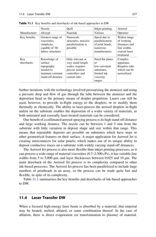
![During ablation, a gas or plasma is formed, which expands rapidly as further laser
energy is added. This rapid expansion can create a shock wave within a material or
it can propel a material. By focusing the expansion of the material during ablation
(utilizing shock waves produced by laser ablation) or taking advantage of rapid
thermal expansion inherent with laser heating, materials can be accurately trans-
ferred in a very repeatable and accurate manner from one location to another. Laser
transfer DW makes use of these phenomena by transferring material from a foil,
tape, or plate onto a substrate. By carefully controlling the energy and location of
the impinging laser, complex patterns of transferred material can be formed on a
substrate.
Two different mechanisms for laser transfer are illustrated in Fig. 11.5.
Figure 11.5a illustrates a laser transfer process where a transparent carrier (a foil
or plate donor substrate which is transparent to the laser wavelength) is coated with
a sacrificial transfer material and the dynamic release layer (the build material). The
impinging laser energy ablates the transfer material (forming a plasma or gas),
which propels the build material towards the substrate. The material impacts the
substrate and adheres, forming a coating on the substrate. When using a pulsed
laser, a precise amount of material can be deposited per pulse.
Figure 11.5b shows a slightly different mechanism for material transfer. In this
case the laser pulse ablates a portion of the surface of a foil. This ablation and
absorption of thermal energy creates thermal waves and shock waves in the
material. These waves are transmitted through the material and cause a portion of
the material on the opposing side to fracture from the surface in a brittle manner
(known as spallation). The fractured material is propelled towards the substrate,
forming a deposit coating on the substrate (not shown).
The Matrix-Assisted Pulsed Laser Evaporation Direct Write (MAPLE-DW)
process was developed to make use of these laser transfer phenomena [12]. A
schematic of the MAPLE-DW process is shown in Fig. 11.6. In this process, a laser
transparent quartz disc or polymer tape is coated on one side with a film (a few
Fig. 11.5 (a) Mechanism for laser transfer using a sacrificial transfer material (based on [10]). (b)
Mechanism for laser transfer using thermal shock and spallation (based on [11]) (courtesy Douglas
B. Chrisey)
278 11 Direct Write Technologies](https://image.slidesharecdn.com/1-230308091212-68402451/85/1-Additive-manufacturing-pdf-296-320.jpg)
![microns thick), which consists of a powdered material that is to be deposited and a
polymer binder. The coated disc or tape is placed in close proximity and parallel to
the substrate. A laser is focused onto the coated film. When a laser pulse strikes the
coating, the polymer is evaporated and the powdered material is deposited on
the substrate, firmly adhering to it. By appropriate control of the positions of both
the ribbon and the substrate, complex patterns can be deposited. By changing the
type of ribbon, multimaterial structures can be produced.
Laser transfer processes have been used to create deposits of a wide variety of
materials, including metals, ceramics, polymers, and even living tissues. The main
drawbacks of a laser transfer process are the need to form a tape with the appropri-
ate transfer and/or deposit materials, and the fact that the unused portions of the tape
are typically wasted.
The benefits of the laser transfer process are that it produces a highly repeatable
deposit (the deposit is quantized based on the laser pulse energy), it can be as
accurate as the laser scanners used to manipulate the laser beam, and the deposited
materials may not need any further post-processing. In addition, the laser can be
used to either simply propel the material onto the substrate without thermally
affecting the substrate or it can be used to laser treat the deposit (including heating,
cutting, etc.) to modify the properties or geometry of the deposit during or after
deposition. In the case of a rigid tape (such as when using a glass plate) the plate is
typically mechanically suspended above the substrate. When a flexible polymer
Fig. 11.6 Matrix-Assisted Pulsed Laser Evaporation Direct Write (MAPLE-DW) process [13]
(Courtesy PennWell Corp., Laser Focus World)
11.4 Laser Transfer DW 279](https://image.slidesharecdn.com/1-230308091212-68402451/85/1-Additive-manufacturing-pdf-297-320.jpg)
![tape is used, it can be laid directly onto the substrate before laser processing and
then peeled from the substrate after laser processing, leaving behind the desired
pattern.
11.5 Thermal Spray DW
Thermal spray is a process that accelerates material to high velocities and deposits
them on a substrate, as shown in Fig. 11.7. Material is introduced into a combustion
or plasma flame (plume) in powder or wire form. The plume melts and imparts
thermal and kinetic energy to the material, creating high-velocity droplets. By
controlling the plume characteristics and material state (e.g., molten or softened)
it is possible to deposit a wide range of metals, ceramics, polymers, or composites
thereof. Particles can be deposited in a solid or semisolid state, which enables the
creation of useful deposits at or near room temperature. Thermal spray techniques
for DW have been commercialized by MesoScribe Technologies, Inc. [14].
A deposit is built-up by successive impingement of droplets, which yield
flattened, solidified platelets, referred to as splats. The deposit microstructure, and
thus its properties, strongly depends on the processing parameters utilized. Key
characteristics of thermal spray DW include: (1) a high volumetric deposition rate,
(2) material flexibility, (3) useful material properties in the as-deposited state
(without thermal treatment or curing), and (4) moderate thermal input during
processing, allowing for deposition on a variety of substrates.
Fig. 11.7 General apparatus for thermal spray [15] (Courtesy of and (C) Copyright Sulzer Metco.
All rights reserved)
280 11 Direct Write Technologies](https://image.slidesharecdn.com/1-230308091212-68402451/85/1-Additive-manufacturing-pdf-298-320.jpg)
![DW thermal spray differs from traditional thermal spray in that the size and
shape of the deposit is controlled by a unique aperture system. A schematic aperture
system from an issued patent is shown in Fig. 11.8. This aperture is made up of
adjustable, moving metal foils (702a and 702b moving horizontally and 708a and
708b moving vertically) which constrain the plume to desired dimensions (region
720). The distance between the moving foils determines the amount of spray which
reaches the substrate. The foils are in constant motion to avoid overheating and
build-up of the material being sprayed. The used foils become a waste product of
the system.
Because the temperature of the substrate is kept low and no post-treatment is
typically required, DW thermal spray is well-suited to produce multilayer devices
formed from different materials. It is possible to create insulating layers, conduc-
tive/electronic layers, and further insulating layers stacked one on top of the other
(including vias for signal transmission between layers) by changing between
various metal, ceramic, and polymer materials. DW thermal spray has been used
to successfully fabricate thermocouples, strain gages, antennas, and other devices
for harsh environments directly from precursor metal and ceramic powders. In
addition, DW thermal spray, combined with ultrafast laser micromachining, has
been shown to be capable of fabricating thermopiles for power generation [16].
Fig. 11.8 Schematic aperture apparatus for direct write thermal spray (US patent 6576861). Foils
702a, b and 708a, b are in constant motion and are adjusted to allow different amounts of spray to
reach the substrate through hole 720 in the center
11.5 Thermal Spray DW 281](https://image.slidesharecdn.com/1-230308091212-68402451/85/1-Additive-manufacturing-pdf-299-320.jpg)
![11.6 Beam Deposition DW
Several direct write procedures have been developed based upon vapor deposition
technologies using, primarily, thermal decomposition of precursor gases. Vapor
deposition technologies produce solid material by condensation, chemical reaction,
or conversion of material from a vapor state. In the case of chemical vapor
deposition (CVD), thermal energy is utilized to convert a reactant gas to a solid
at a substrate. In the regions where a heat source has raised the temperature above a
certain threshold, solid material is formed from the surrounding gaseous precursor
reactants. The chemical composition and properties of the deposit are related to the
thermal history during material deposition. By moving a localized heat source
across a substrate (such as by scanning a laser) a complex geometry can be formed.
A large number of research groups over almost 20 years have investigated the use of
vapor deposition technologies for additive manufacturing purposes [17]. A few
examples of these technologies are described below.
11.6.1 Laser CVD
Laser Chemical Vapor Deposition (LCVD) is a DW process which uses heat from a
laser to selectively transform gaseous reactants into solid materials. In some
systems, multiple gases can be fed into a small reactant chamber at different
times to form multimaterial structures, or mixtures of gases with varying
concentrations can be used to form gradient structures. Sometimes flowing jets of
gas are used to create a localized gaseous atmosphere, rather than filling a chamber
with the gaseous precursor materials.
The resolution of an LCVD deposit is related to the laser beam diameter, energy
density, and wavelength (which directly impact the size of the heated zone on the
substrate) as well as substrate thermal properties. Depending on the gases present at
the heated reactive zone, many different metals and ceramics can be deposited,
including composites. LCVD has been used to deposit carbon fibers and multilay-
ered carbon structures in addition to numerous types of metal and ceramic
structures.
A LCVD system developed at the Georgia Institute of Technology is displayed
in Fig. 11.9. This design constrains the reactant gas (which is often highly corrosive,
and/or biologically harmful) to a small chamber that is separated from the motion
controllers and other mechanisms. This small, separated reaction chamber has
multiple benefits, including an ability to quickly change between reagent gas
materials for multimaterial deposition, and better protection of the hardware from
corrosion. By monitoring the thermal and dimensional characteristics of the
deposit, process parameters can be controlled to create deposits of desired geometry
and material properties.
LCVD systems are capable of depositing many types of materials, including
carbon, silicon carbide, boron, boron nitride, and molybdenum onto various
substrates including graphite, grafoil, zirconia, alumina, tungsten, and silicon
282 11 Direct Write Technologies](https://image.slidesharecdn.com/1-230308091212-68402451/85/1-Additive-manufacturing-pdf-300-320.jpg)
![[18]. Direct write patterns as well as fibers have been successfully deposited. A
wide variety of materials and deposit geometries make LCVD a viable technology
for further direct write developments. LCVD is most comparable to microthermal
spray, in that deposits of metals and ceramics are directly formed without post-
treatment, but without the “splat” geometry inherent in thermal spray. The benefits
of LCVD are the unique materials and geometries it can deposit. However, LCVD
has a very low deposition rate and a relatively high system complexity and cost
compared to most DW approaches (particularly ink-based technologies). High-
temperature deposition can be another disadvantage of the process. In addition,
the need to deposit on surfaces that are contained within a controlled-atmosphere
chamber limits its ability to make deposits on larger preexisting structures.
LCVD can be combined with layer-wise deposition of powders (similar to the
binder jetting techniques in Chap. 8) to more rapidly fabricate structures than when
using LCVD alone. In this case the solid material created from the vapor phase is
used to bind the powdered material together in regions where the laser has heated
the powder bed. This process is known as Selective Area Laser Deposition Vapor
Infiltration (SALDVI). In SALDVI, the build-rates are much higher than when the
entire structure is fabricated from LCVD-deposited materials only; but the resultant
Fig. 11.9 The LCVD system developed at Georgia Tech
11.6 Beam Deposition DW 283](https://image.slidesharecdn.com/1-230308091212-68402451/85/1-Additive-manufacturing-pdf-301-320.jpg)
![structures may be porous and are composite in nature. The build-rate difference
between LCVD and SALDVI is analogous to the difference between binder jetting
and material jetting.
11.6.2 Focused Ion Beam CVD
A focused ion beam (FIB) is a beam of ionized gallium atoms created when a
gallium metal source is placed in contact with a tungsten needle and heated. Liquid
gallium wets the needle, and the imposition of a strong electric field causes
ionization and emission of gallium atoms. These ions are accelerated and focused
in a small stream (with a spot size as low as a few nanometers) using electrostatic
lenses. A FIB is similar in conceptualization to an electron beam source, and thus
FIB is often combined with electron beams, such as in a dual-beam FIB-scanning
electron microscope system.
FIB processing, when done by itself, can be destructive, as high-energy gallium
ions striking a substrate will cause sputtering and removal of atoms. This enables
FIB to be used as a nanomachining tool. However, due to sputtering effects and
implantation of gallium atoms, surfaces near the machining zone will be changed
by deposition of the removed material and ion implantation. This sputtering and ion
implantation, if properly controlled, can also be a benefit for certain applications.
Direct write deposition using FIB is possible in a manner similar to LCVD. By
scanning the FIB source over a substrate in the presence of CVD gaseous
precursors, solid materials are deposited onto the substrate (and/or implanted within
the surface of the substrate) [19, 20]. These deposits can be submicron in size and
feature resolution. FIB CVD for DW has been used to produce combinations of
metallic and dielectric materials to create three-dimensional structures and cir-
cuitry. In addition, FIB CVD is being used in the integrated circuits (IC) industry
to repair faulty circuitry. Both the machining and deposition features of FIB are
used for IC repairs. In the case of short-circuits, excess material can be removed
using a FIB. In the case of improperly formed electrical contacts, FIB CVD can be
used to draw conductive traces to connect electrical circuitry.
11.6.3 Electron Beam CVD
Electron beams can be used to induce CVD in a manner similar to FIB CVD and
LCVD. Electron beam CVD is slower than laser or FIB CVD; however, FIB CVD
and electron beam CVD both have a better resolution than LCVD [21].
284 11 Direct Write Technologies](https://image.slidesharecdn.com/1-230308091212-68402451/85/1-Additive-manufacturing-pdf-302-320.jpg)
![11.7 Liquid-Phase Direct Deposition
Similarly to the vapor techniques described above, thermal or electrical energy can
be used to convert liquid-phase materials into solid materials. These thermochemi-
cal and electrochemical techniques can be applied in a localized manner to create
prescribed patterns of solid material.
Drexel University illustrated the use of thermochemical means for DW traces
using ThermoChemical Liquid Deposition (TCLD). In TCLD, liquid reactants are
sprayed through a nozzle onto a hot substrate. The reactants thermally decompose
or react with one another on the hot surface to form a solid deposit on the substrate.
By controlling the motion of the nozzle and the spraying parameters, a 3D shape of
deposited material can be formed. This is conceptually similar to the ink-based DW
approaches discussed above, but requires a high-temperature substrate during
deposition.
A second Electrochemical Liquid Deposition (ECLD) approach was also tested
at Drexel. In ECLD, a conductive substrate is submerged in a plating bath and
connected to a DC power source as the cathode, as in Fig. 11.10. A pin made up of
the material to be deposited is used as the anode. By submerging the pin in the bath
near the substrate and applying an appropriate voltage and current, electrochemical
decomposition and ion transfer results in a deposit of the pin material onto the
substrate. By moving the pin, a prescribed geometry can be traced. As electrochem-
ical plating is a slow process, the volumetric rate of deposition for ELCD can be
increased by putting a thin layer of metal powder in the plating bath on the surface
of the substrate (similar conceptually to SALDVI described above). In this case, the
Fig. 11.10 Schematic of an electrochemical liquid deposition system [22] (MATERIALS
DESIGN by Zongyan He, Jack G. Zhou and Ampere A. Tseng. Copyright 2000 by Elsevier
Science Technology Journals. Reproduced with permission of Elsevier Science Technology
Journals in the format Textbook via Copyright Clearance Center.)
11.7 Liquid-Phase Direct Deposition 285](https://image.slidesharecdn.com/1-230308091212-68402451/85/1-Additive-manufacturing-pdf-303-320.jpg)
![deposited material acts as a binder for the powdered materials, and the volumetric
rate of deposition is significantly increased [22].
Thermochemical and electrochemical techniques can be used to produce
complex-geometry solids at small length scales from any metal compatible with
thermochemical or electrochemical deposition, respectively. These processes are
also compatible with some ceramics. However, these approaches are not available
commercially and may have few benefits over the other DW techniques described
above. Drawbacks of TCLD-based approaches are the need for a heated substrate
and the use of chemical precursors which may be toxic or corrosive. Drawbacks of
ECLD-based approaches include the slow deposition rate of electrochemical pro-
cesses and the fact that, when used as a binder for powders, the resultant product is
porous and requires further processing (such as sintering or infiltration) to achieve
desirable properties.
11.8 Beam Tracing Approaches to Additive/Subtractive DW
By combining layer-wise additive approaches with freeform beam (electron, FIB,
or laser) subtractive approaches, it is possible to create DW features. Many coating
techniques exist to add a thin layer of material to a substrate. These include physical
vapor deposition, electrochemical or thermochemical deposition, CVD, and other
thin film techniques used in the fabrication of integrated circuits. Once these layers
are added across the surface of a substrate, a beam can be used to trim each layer
into the prescribed cross-sectional geometry. These micro- or nanodiameter beams
are used to selectively cure or remove materials deposited in a layer-by-layer
fashion. This approach is conceptually similar to the bond-then-form sheet lamina-
tion techniques discussed in Chap. 9.
11.8.1 Electron Beam Tracing
Electron beams can be used to either cure or remove materials for DW. Standard
spin-on deposition coating equipment can be used to produce thin films between
30 and 80 nm. These films are then exposed to a prescribed pattern using an electron
beam. Following exposure, the uncured material is removed using standard
IC-fabrication techniques. This methodology can produce line-edge definition
down to 3.3 nm. A converse approach can also be used, whereby the exposed
material is removed and the unexposed material remains behind. In the case of
curing, low-energy electrons can be utilized (and are often considered more desir-
able, to reduce the occurrence of secondary electron scattering). These techniques
fit well within existing IC-fabrication methodologies and enable maskless IC
fabrication.
Another variant of electron beam tracing is to produce a thin layer of the desired
material using physical vapor deposition or a similar approach and then to use high-
286 11 Direct Write Technologies](https://image.slidesharecdn.com/1-230308091212-68402451/85/1-Additive-manufacturing-pdf-304-320.jpg)
![powered electron beams to remove portions of the coating to form the desired
pattern.
Electron beams are not particularly efficient for either curing or removing layers
of material, however. Thus, electron beam tracing techniques for DW are
quite slow.
11.8.2 Focused Ion Beam Tracing
As discussed above, a FIB can be utilized to machine materials in a prescribed
pattern. By combining the steps of layer-wise deposition with FIB machining, a
multilayer structure can be formed. If the deposited material is changed layer-by-
layer, then a multimaterial or gradient structure can be formed.
11.8.3 Laser Beam Tracing
Short-wavelength lasers can be utilized to either cure layers of deposited materials
or ablatively remove materials to form micro and nanoscale DW features. To
overcome the diffraction limit of traditional focusing optics, a number of
nanopatterning techniques have been developed to create features that are smaller
than half the optical wavelength of the laser [23]. These techniques include
multiphoton absorption, near-field effects, and Bessel beam optical traps. Although
these techniques can be used to cure features at the nano scale, inherent problems
with alignment and positioning at these length scales make it difficult to perform
subwavelength nanopatterning in practice.
These laser approaches are conceptually identical to the electron beam and
FIB-based additive plus subtractive approaches just mentioned. Some of the
benefits of lasers for beam tracing DW are that they can process materials much
more rapidly than electron beams, and they can do so without introducing FIB
gallium ions. The main drawback of lasers is their relatively large spot size
compared to electron and FIBs.
11.9 Hybrid Technologies
As in most additive manufacturing techniques, there is an inherent trade-off
between material deposition speed and accuracy for most DW processes. This
will remain true until techniques are developed for line-wise or layer-wise deposi-
tion (such as is done with mask projection stereolithography using a DLP system, as
described in Chap. 4). Thus, to achieve a good combination of deposition speed and
accuracy, hybrid technologies are often necessary. Some examples of hybrid
technologies have already been mentioned. These include the additive/subtractive
beam tracing methods described above and the use of a laser in the Aerosol Jet
aerosol system.
11.9 Hybrid Technologies 287](https://image.slidesharecdn.com/1-230308091212-68402451/85/1-Additive-manufacturing-pdf-305-320.jpg)
![The primary form of hybrid technology used in DW is to form deposits quickly
and inexpensively using an ink-based technique and then trim those deposits using a
short-wavelength laser. This results in a good combination of build speed, accuracy,
and overall cost for a wide variety of materials. In addition, the laser used to trim the
ink-based deposits has the added benefit of being an energy source for curing the
deposited inks, when used in a lower power or more diffuse manner. If DW is
integrated with an AM process that includes a laser, such as stereolithography, the
laser can be used to modify the DW traces [24].
One of the fastest hybrid DW approaches is the “roll-to-roll” approach. As the
name suggests, roll-to-roll printing is analogous to high-speed 2D printing. In roll-
to-roll DW, a paper or plastic sheet of material is used as a substrate material and
moved through printing rolls that deposit patterns of DW ink that are subsequently
thermally processed, such as with a flash lamp. Inkjet printing and other DW
techniques can be added into the roll-to-roll facility to add ink patterns in a more
flexible manner than the repeated patterns printed by a printing roll. When DW
techniques and flexible laser systems are integrated into a roll-to-roll facility, this
gives the combination of the speed of line-wise AM via the rolls plus the flexibility
of point-wise AM via another DW technique.
11.10 Applications of Direct Write Technologies
The applications of DW processes are growing rapidly [25]. There is a growing
variety of materials which are available, including semiconductors, dielectric
polymers, conductive metals, resistive materials, piezoelectrics, battery elements,
capacitors, biological materials, and others. These can be deposited onto various
substrate materials including plastic, metal, ceramic, glass, and even cloth. The
combination of these types of materials and substrates means that the applications
for DW are extremely broad.
The most often cited applications for DW techniques are related to the fabrica-
tion of sensors. DW approaches have been used to fabricate thermocouples,
thermistors, magnetic flux sensors, strain gages, capacitive gages, crack detection
sensors, accelerometers, pressure gages, and more [3, 14, 16, 26].
A second area of substantial interest is in antenna fabrication. Since DW, like
other AM techniques, enables fabrication of complex geometries directly from
CAD data, antenna designs of arbitrary complexity can be made on the surface of
freeform objects; including, for instance, fractal antennas on conformal surfaces.
Figure 11.11 illustrates the fabrication of a fractal antenna on the abdomen of a
worker honeybee using MAPLE-DW.
Another area of interest for DW is as a freeform tool to connect combinations of
electronic components on freeform surfaces. One area where this is particularly
useful is in harsh environments, as shown in Fig. 11.12. In this example, direct write
thermal spray is used as a method for producing and connecting a series of
electronic components that monitor and feed back information about the state of
a turbine blade. A thermocouple, labeled High-Temperature Sensor in the figure, is
288 11 Direct Write Technologies](https://image.slidesharecdn.com/1-230308091212-68402451/85/1-Additive-manufacturing-pdf-306-320.jpg)
![deposited on the hot region of the blade, whereas the supporting electronics are
deposited on the cold regions of the blade. DW-produced conductors are used to
transmit signals between regions and components.
Although most DW processes can produce thermal and strain sensors, there is
still opportunity for improved conductors, insulators, antennas, batteries,
capacitors, resistors, and other electronic circuitry. In addition, in every case
where a conductive path is not possible between a power source and a deposited
sensor, some form of local power generation is necessary. Several researchers have
demonstrated the ability to create systems which use electromagnetic or thermopile
power generation schemes using DW [16]. If designs for energy harvesting devices
Fig. 11.11 35-GHz fractal antenna design (left) and MAPLE-DW printed antenna on the
abdomen of a dead drone honeybee (right). (Courtesy Douglas B. Chrisey)
Fig. 11.12 A direct write
sensor and associated wiring
on a turbine blade structure.
Signal conditioning
electronics are positioned on a
more shielded spot (Courtesy
MesoScribe Technologies,
Inc. and Arkansas Power
Electronics Int.)
11.10 Applications of Direct Write Technologies 289](https://image.slidesharecdn.com/1-230308091212-68402451/85/1-Additive-manufacturing-pdf-307-320.jpg)
![differing markets. For most of these markets, the more successful vendors also
ensured they had excellent intellectual property (IP) protection. All of this served to
maintain the technology at a high cost.
Ultimately it was the issues surrounding IP that led to the current situation. Many
of the original technologies were protected by patents that prevented other
companies from copying them. The vendor companies were also very aggressive
in defending their IP as well as buying up related IP and their associated companies
where they existed. This competitive market did have the effect of slowly eroding
the vendor companies’ profit margins, but huge changes have recently taken place
as a result of these patents lapsing. We will go on in this chapter to discuss how this
has impacted the low-cost AM technology marketplace. The key patents will be
discussed as well as the more prominent players in this field. This activity has
fuelled a huge amount of interest by the media, which will be discussed in terms of
how it has in turn impacted the industry. Much of this interest can be associated
with what is becoming known as disruptive innovation. AM certainly fits with a
number of other technologies to form the basis for disruptive business models,
which we will discuss. AM also is a huge enabling technology that has assisted
many home users to solve many of their own technical problems at home. Sharing
these experiences and even profiting from them has spearheaded what is being
commonly called the Maker Movement, which we shall also examine. We will go
on to consider how this branch of AM may develop in the future.
12.2 Intellectual Property
As mentioned in the introduction and in other parts of this book, the key patents
with the most protection originated in the USA. While there was activity in other
countries, 3D Systems, Stratasys, DTM, and Helisys were the principal vendor
names for much of the world in the early days. Other companies were also present,
like EOS, Sony, Sanders, and Objet, but they either came along at a later date or
were in close IP conflict with these American vendors.
European and US patent law for technology are somewhat similar to each other
in that they refer to a 20-year term from the initial filing date of the patent in most
cases. Charles Hull filed his first Stereolithography patent in 1984 [1], which
therefore expired in 2004. Scott Crump patented the Fused Deposition Modeling
process in 1989 [2], which means that patent expired in 2009. The major difference
between these technologies, in this context, is that the melt extrusion process is
much easier to replicate at a low cost compared with the laser-cured photopolymer
systems. It is evident therefore that while the door to widespread development was
opened in 2004, it was not opened wide until 2009 and beyond. This is evident from
the figures quoted by Terry Wohlers from 2008 to 2013, shown in Fig. 12.1,
concerning the number of low-cost AM machines purchased over that period [3].
Of course this is not the complete story. While the original patents were filed in
the 1980s, additional patents have been constantly filed ever since. If one notices
that there have been many copies of the original FDM patent, all the resulting
294 12 The Impact of Low-Cost AM Systems](https://image.slidesharecdn.com/1-230308091212-68402451/85/1-Additive-manufacturing-pdf-311-320.jpg)
![machines have thus far not implemented an environmental control apparatus. This
is because the patent for this development was not filed by Crump until a few years
later.
There is an excellent review of the recently expiring and shortly expiring patents
carried out by Hornick and Roland [4]. In it they make a number of interesting
observations that lead to the following discussion:
– There is a huge number of patents involved and it is a very difficult process to
navigate through them. Many patents make multiple claims across numerous
platforms. They often do not adhere to a single process.
– Earlier patents discuss broad-based approaches that are in fact quite easy to
defend and/or find ways around. It is quite easy to distinguish one process from
another since they do not have the benefits that are gained through experience of
actual application of the technology. Later patents obviously result from
discoveries resulting from use of these base technologies, which discuss subtle
features like soluble supports or fill patterns.
– While 3D Systems patents are among the earliest to expire, there are obvious
technical complexities in them that would make them difficult to replicate
without significant industrial backing. An example relates to the formulation
of resins to speed up the curing and build process or another to facilitate even
spreading of resins.
2008
355 1816
5978
24265
35508
72503
0
10000
20000
30000
40000
50000
60000
70000
80000
2009 2010 2011 2012 2013
Fig. 12.1 Wohlers’ data showing how the numbers of low-cost AM machines has increased from
virtually nothing in 2008
12.2 Intellectual Property 295](https://image.slidesharecdn.com/1-230308091212-68402451/85/1-Additive-manufacturing-pdf-312-320.jpg)
![– Some key droplet deposition and powder sintering by laser patents expired in
late 2014, early 2015. Expiration of these patents may help to open up the high-
end, high-quality AM market by bringing the machine costs down.
At the time of writing this chapter it is merely speculation, but it will be
interesting to see how some of the large printing or equipment manufacturing
companies view these as opportunities. One can anticipate that a large printer
company may possess the necessary knowledge, resources, and infrastructure to
produce high-quality AM equipment in volume at very reasonable costs. It is worth
noting that although low-cost AM started with material extrusion technology, since
they were the easiest to produce and some of the first patents to expire, low-cost
versions of photopolymerization (Formlabs), polymer laser sintering (Norge), and
even metal machines such as metal laser sintering (Matterfab) and lower-cost
directed energy deposition heads (Hybrid Manufacturing Technologies or the
LENS print engine) are starting to proliferate.
12.3 Disruptive Innovation
12.3.1 Disruptive Business Opportunities
Disruptive innovation and disruptive technology are terms that were originally
defined by Christensen to describe activities or technology that create new markets
[5]. A very obvious example of this is how the Internet made it possible to create
online businesses which could not have existed before. However, the effects may be
much more subtle and it is possible to create a disruptive business merely by using
existing technology in a different way. Often this process can be achieved by early
adopters of technology or by those who have skills that are either difficult to learn or
not commonly used in a disruptive way. Here we can say that although there are
many musicians, there is only one David Bowie or Lady Gaga, who made use of
their artistic talents to generate additional business opportunities.
There is no doubt that AM is a disruptive technology, which can be combined
with other technologies to generate new businesses. Improvements and more
widespread use of CAD technology has made it possible for individuals to design
products with minimal cost and training. Google Sketchup and Tinkercad are online
design tools that are basically free to use. While they are not as powerful and
versatile as paid CAD software, these accessible and simple to use tools have
opened up a new market for home designers, who would then like to find outlets
for these designs. While eventually this may mean all of these people will have
machines in their homes, we are not quite there yet. Some people may have a
low-cost AM machine at home, but even these may not meet the functional
requirements and so will look to outside services to build and supply their designs.
This has led to the establishment of companies who provide online services where
designers can not only have their models made but also find an outlet where their
designs can also be sold. Shapeways and i.materialise (see Fig. 12.2) both operate in
296 12 The Impact of Low-Cost AM Systems](https://image.slidesharecdn.com/1-230308091212-68402451/85/1-Additive-manufacturing-pdf-313-320.jpg)
![this space, using techniques developed for social media platforms, where viewers
can “like” other people’s designs as well as discuss, share, and promote them. For
those wishing to share designs but not concerned with the commercial aspects, there
are also portals like the Thingiverse web site. Issues surrounding copyright of
designs are regularly discussed around these web sites. Replicas or models inspired
by merchandising for TV and movie shows for example can be regularly found on
these sites and some sharing sites will have more or less control than others.
12.3.2 Media Attention
Since disruptive innovation is always going to attract media attention, it is worth
considering some of the more prominent stories that have attracted interest and
therefore structured how the general public view AM.
The first example that springs to many people’s minds would be the use of AM to
create firearms. A great deal of attention was directed towards AM when it was
realized that it was possible to create firearms using the technology, the most well-
known of these being the Liberator, single-shot pistol [6]. Here, it was discovered
that this gun could be largely manufactured using an AM machine and that the plans
for its manufacture were posted online. A primary reason for this attracting so much
attention was the obvious contentious nature of the topic, backed up by the fact that
this design can be easily shared on the Internet. It was particularly interesting to
note that the attention was focused on the negative impact of AM rather than that of
the Internet. There are a number of issues that are worth discussing here:
Fig. 12.2 Web site image for i.materialise, showing how designers can post their ideas on the web
and have them built and made available for others to buy
12.3 Disruptive Innovation 297](https://image.slidesharecdn.com/1-230308091212-68402451/85/1-Additive-manufacturing-pdf-314-320.jpg)
![– While the gun was indeed built, certain items like the firing pin and obviously
the ammunition would need to be added to the design.
– The original gun was created using a relatively high-end AM machine by a
skilled operator. Sharing of the design online does not include the build
parameters and a study by the New South Wales police in Australia revealed
that the user is at great risk if the gun is not built correctly [7].
– Improvised firearms have been possible for many years and can be constructed
by anyone with a small amount of technical knowledge and access to simple
manufacturing equipment [8].
Admittedly, AM can be used like any technology, for good or for bad. However,
we can see here how the media can latch on to one example and confuse the public
image. These examples did bring the technology into a much wider public domain
than previously and therefore allowed specialists in the field the opportunity to
more properly explain the true impact of AM.
In stark contrast to the use of AM for destructive purposes, there have been
numerous articles that describe how AM can be used to create replacement body
parts [9]. As described in the chapter on Applications in this book, there is a huge
potential for AM to contribute in this direction. The problem in the media coverage
however is the time frame attached to this. Some applications have been
implemented where AM has made significant improvements in medical and
healthcare. However, this cannot be easily generalized into a conclusion that all
medical problems can be solved this way. We must expect significant developments
in the technology before we can make that conclusion and the AM machines of the
future will look nothing like the machines we have today. Furthermore, we need
parallel efforts in the biomedical sciences as well because they are far from being
ready to plug in directly to AM devices. Specialists in these fields need to under-
stand that, while it is reasonable to speculate that AM for body parts is on the
horizon, they must be wary of that message being misconstrued.
Another sector that has attracted the media attention is the “cool gadget” area.
One early example that again elevated general public awareness was The Econo-
mist magazine front-page article titled “Print me a Stradivarius” (see Fig. 12.3).
This was probably the first mass-market article that highlighted how AM could be
used for truly functional applications. While other media sites have included similar
articles somewhere in their portfolios, the fact that this was on the front-page of an
international magazine certainly had an impact. It is also worthwhile taking note
that the BBC have published regular articles about AM over the years, averaging
around 1 every 2 months or so in a wide variety of areas.
In relation to this chapter, the reason for including these articles is because of the
increasing number of personal users of AM machines. All of these articles have one
thing in common: they imply that you will eventually be able to create solutions for
yourself.
298 12 The Impact of Low-Cost AM Systems](https://image.slidesharecdn.com/1-230308091212-68402451/85/1-Additive-manufacturing-pdf-315-320.jpg)
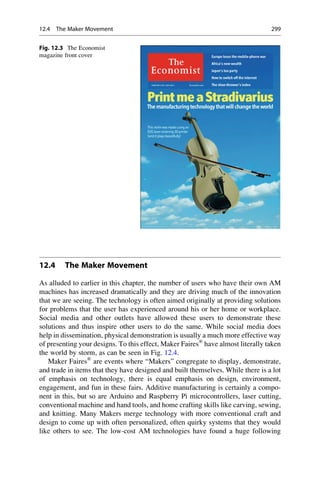
![within this Maker movement that is fuelling a large amount of innovation and even
spinning off into new commercial ventures.
Perhaps not surprisingly this Maker movement originated in the USA, originally
promoted by Make magazine [10] for the first event in California in 2006. The USA
has a long and distinguished culture of innovation, perhaps spawning from the
original frontier mentality of having to make do with whatever is around you, and
this can also be seen in terms of how innovation is an accepted part of everyday life
there. However, the concept of the fair is now a worldwide phenomenon with
dozens of events held yearly attracting thousands of exhibitors and hundreds of
thousands of attendees. The Maker Faire®
has become the spiritual home for the
Makerbot and other similar low-cost AM technologies, including the RepRap
designs [11], and for design sharing portals like Thingiverse.
A huge number of commercial entry-level machines can thank the RepRap
project for their origins. It would be almost impossible to identify every company,
there are so many with varying levels of success. Designs have evolved consider-
ably from the original RepRap machines, but the basic principle remains very much
the same, exploiting the hot-melt extrusion process that was facilitated by the FDM
patent expiry.
The Maker movement, along with the FabLab [12] and Idea to Product (I2P [13])
concepts, has done much to highlight the benefits of AM and associated
technologies to the general public. The FabLab and the I2P labs are walk-in
facilities aimed at providing an environment that encourages people to experiment
with accessible manufacturing technologies and develop their ideas. Often the costs
are at least partially absorbed by local authorities or donations. These are different
from what is referred to as hardware incubators, where the costs are sourced from an
investor network. All of these recognize in some way that there is a need to foster
the creative processes.
Fig 12.4 Maker Faire web page
300 12 The Impact of Low-Cost AM Systems](https://image.slidesharecdn.com/1-230308091212-68402451/85/1-Additive-manufacturing-pdf-317-320.jpg)
![Guidelines for Process Selection
13
Abstract
AM processes, like all materials processing, are constrained by material
properties, speed, cost, and accuracy. The performance capabilities of materials
and machines lag behind conventional manufacturing technology (e.g., injection
molding machinery), although the lag is decreasing. Speed and cost, in terms of
time to market, are where AM technology contributes, particularly for complex
or customized geometries.
13.1 Introduction
The initial purpose of rapid prototyping technology was to create parts as a means
of visual and tactile communication. Since those early days of rapid prototyping,
the applications of additive manufacturing processes have expanded considerably.
According to Wohlers and Associates [1], parts from AM machines are used for a
number of purposes, including:
• Visual aids
• Presentation models
• Functional models
• Fit and assembly
• Patterns for prototype tooling
• Patterns for metal castings
• Tooling components
• Direct digital/rapid manufacturing
AM processes, like all materials processing, are constrained by material
properties, speed, cost, and accuracy. The performance capabilities of materials
and machines lag behind conventional manufacturing technology (e.g., injection
molding machinery), although the lag is decreasing. Speed and cost, in terms of
# Springer Science+Business Media New York 2015
I. Gibson et al., Additive Manufacturing Technologies,
DOI 10.1007/978-1-4939-2113-3_13
303](https://image.slidesharecdn.com/1-230308091212-68402451/85/1-Additive-manufacturing-pdf-319-320.jpg)
![time to market, are where AM technology contributes, particularly for complex or
customized geometries.
With the growth of AM, there is going to be increasing demand for software that
supports making decisions regarding which machines to use and their capabilities
and limitations for a specific part design. In particular, software systems can help in
the decision-making process for capital investment of new technology, providing
accurate estimates of cost and time for quoting purposes, and assistance in process
planning.
This chapter deals with three typical problems involving AM that may benefit
from decision support:
1. Quotation support. Given a part, which machine and material should I use to
build?
2. Capital investment support. Given a design and industrial profile, what is the
best machine that I can buy to fulfill my requirements?
3. Process planning support. Given a part and a machine, how do I set it up to work
in the most efficient manner alongside my other operations and existing tasks?
Examples of systems designed to fulfill the first two problems are described in
detail. The third problem is much more difficult and is discussed briefly.
13.2 Selection Methods for a Part
13.2.1 Decision Theory
Decision theory has a rich history, evolving in the 1940s and 1950s from the field of
economics [2]. Although there are many approaches taken in the decision theory
field, the focus in this chapter will be only on the utility theory approach. Broadly
speaking, there are three elements of any decision [3]:
• Options—the items from which the decision maker is selecting
• Expectations—of possible outcomes for each option
• Preferences—how the decision maker values each outcome
Assume that the set of decision options is denoted as A ¼ {A1, A2,. . .,An}. In
engineering applications, one can think of outcomes as the performance of the
options as measured by a set of evaluation criteria. More specifically, in AM
selection, an outcome might consist of the time, cost, and surface finish of a part
built using a certain AM process, while the AM process itself is the option.
Expectations of outcomes are modeled as functions of the options, X ¼ g(A), and
may be modeled with associated uncertainties.
Preferences model the importance assigned to outcomes by the decision maker.
For example, a designer may prefer low cost and short turn-around times for a
concept model, while being willing to accept poor surface finish. In many ad hoc
304 13 Guidelines for Process Selection](https://image.slidesharecdn.com/1-230308091212-68402451/85/1-Additive-manufacturing-pdf-320-320.jpg)
![decision support methods, preferences are modeled as weights or importances,
which are represented as scalars. Typically, weights are specified so that they
sum to 1 (normalized). For simple problems, the decision maker may just choose
weights, while for more complex decisions, more sophisticated methods are used,
such as pair-wise comparison [4]. In utility theory, preferences are modeled as
utility functions on the expectations. Expectations are then modeled as expected
utility. The best alternative is the one with the greatest expected utility.
F. Mistree, J.K. Allen, and their coworkers have been developing the Decision
Support Problem (DSP) Technique over the last 20 years. The advantages of DSPs,
compared with other decision formulations, are that they provide a means for
mathematically modeling design decisions involving multiple objectives and
supporting human judgment in designing systems [5, 6]. The formulation and
solution of DSPs facilitate several types of decisions, including:
Selection—the indication of preference, based on multiple attributes, for one
among several alternatives, [7].
Compromise—the improvement of an alternative through modification [4, 6].
Coupled and hierarchical—decisions that are linked together, such as selection–
selection, compromise–compromise, or selection–compromise [6].
The selection problems being addressed in this chapter will be divided into two
related selection subproblems. First, it is necessary to generate feasible alternatives,
which, in this case, include materials and processes. Second, given those feasible
alternatives, a quantification process is applied that results in a rank-ordered list of
alternatives. The first subproblem is referred to as “Determining Feasibility,” while
the second is simply called “Selection.” Additional feasibility determination and
selection methods will be discussed in this section as well.
13.2.2 Approaches to Determining Feasibility
The problem of identifying suitable materials and AM machines with which to
fabricate a part is surprisingly complex. As noted previously, there are many
possible applications for an AM part. For each application, one should consider
the suitability of available materials, fabrication cost and time, surface finish and
accuracy requirements, part size, feature sizes, mechanical properties, resistance to
chemicals, and other application-specific considerations. To complicate matters,
the number and capability of commercial materials and machines continues to
increase. So, in order to solve AM machine and process chain selection problems,
one must navigate the wide variety of materials and machines, comparing one’s
needs to their capabilities, while ensuring that the most up-to-date information is
available.
To date, most approaches to determining feasibility have taken a knowledge-
based approach in order to deal with the qualitative information related to AM
process capability. One of the better developed approaches was presented by Deglin
and Bernard [8]. They presented a knowledge-based system for the generation,
selection, and process planning of production AM processes. The problem as they
13.2 Selection Methods for a Part 305](https://image.slidesharecdn.com/1-230308091212-68402451/85/1-Additive-manufacturing-pdf-321-320.jpg)
![defined it was: “To propose, from a detailed functional specification, different
alternatives of rapid manufacturing processes, which can be ordered and optimized
when considering a combination of different specification criteria (cost, quality,
delay, aspect, material, etc.).” Their approach utilized two reasoning methods, case-
based and the bottom-up generation of processes; the strengths of each
compensated for the other’s weaknesses. Their system was developed on the
KADVISER platform and utilized a relational database system with extensive
material, machine, and application information.
A group at the National University of Singapore (NUS) developed an AM
decision system that was integrated with a database system [9, 10]. Their selection
system was capable of identifying feasible material/machine combinations,
estimating manufacturing cost and time, and determining optimal part orientations.
From the feasible material/machines, the user can then select the most suitable
combination. Their approach to determining feasible materials and processes is
broadly similar to the work of Deglin and Bernard. The NUS group utilized five
databases, each organized in a hierarchical, object-oriented manner: three general
databases (materials, machines, and applications) and two part-specific databases
(geometric information and model specifications).
Several web-based AM selection systems are available. One was developed at
the Helsinki University of Technology (see http://ltk.hut.fi/RP-Selector/). Through
a series of questions, the selector acquires information about the part accuracy,
layer thickness, geometric features, material, and application requirements. The
user chooses one of 4–5 options for each question. Additionally, the user specifies
preferences for each requirement using a 5-element scale from insignificant to
average to important. When all 10–12 questions are answered, the user receives a
set of recommended AM machines that best satisfy their requirements.
The problem of determining process and material feasibility can be represented
by the Preliminary Selection Decision Support Problem (ps-DSP) [11]. The word
formulation of the ps-DSP is given in Fig. 13.1. This is a structured decision
formulation and corresponds to a formal decision method based on decision theory.
Qualitative comparisons among processes and materials, with respect to decision
criteria, are sufficient to identify feasible alternatives and eliminate infeasible ones.
After more quantitative information is known, more detailed evaluations of
alternatives can be made, as described in the next subsection.
Given: a set of concepts
Identify: The principal criteria influencing selection.
The relative importance of the criteria
Capture: Experience-based knowledge about the concepts with respect to a datum and the
established criteria.
Rank: The concepts in order of preference based on multiple criteria and their relative
importance.
Fig. 13.1 Preliminary selection decision support problem word formulation
306 13 Guidelines for Process Selection](https://image.slidesharecdn.com/1-230308091212-68402451/85/1-Additive-manufacturing-pdf-322-320.jpg)
![The key step in the ps-DSP is how to capture and apply experience-based
knowledge. One chooses a datum concept against which all other concepts are
compared. Qualitative comparisons are performed, where a concept is judged as
better, worse, or about the same (+1, 1, 0, respectively) as the datum with respect
to the principal criteria for the selection problem. Then, a weighted sum of
comparisons with the datum is computed. Typically, this procedure is repeated
for several additional choices of datums. In this manner, one gets a good under-
standing of the relative merits and deficiencies of each concept.
The ps-DSP has been applied to various engineering problems, most recently for
a problem to design an AM process to fabricate metal lattice structures [12].
13.2.3 Approaches to Selection
As stated earlier, there have been a number of approaches taken to support the
selection of AM processes for a part. Most aid selection, but only in a qualitative
manner, as described earlier. Several methods have been developed in academia
that are based on the large literature on decision theory. For an excellent introduc-
tion to this topic, see the book by Keeney and Raiffa [2]. In this section, the
selection DSP is covered in some detail and selection using utility theory is
summarized.
While the basic advantages of using DSPs of any type lie in providing context
and structure for engineering problems, regardless of complexity, they also facili-
tate the recording of viewpoints associated with these decisions, for completeness
and future reference, and evaluation of results through post solution sensitivity
analysis. The standard Selection Decision Support Problem (s-DSP) has been
applied to many engineering problems and has recently been applied to AM
selection [13]. The word formulation of the standard s-DSP is given in Fig. 13.2.
Note that the decision options for AM selection are feasible material-process
combinations. Expectations are determined by rating the options against the
attributes. Preferences are modeled using simple importance values. Rank ordering
of options is determined using a weighted-sum expression of importance and
attribute ratings. An extension to include utility theory has recently been accom-
plished, as described next.
For the Identify step, evaluation attributes are to be specified. For example,
accuracy, cost, build time, tensile strength, and feature detail (how small of a
feature can be created) are typical attributes. Scales denote how the attribute is to
Given: Set of AM processes/machines and materials (alternatives)
Identify: Set of evaluation attributes. Create scales and determine importances.
Rate: Each alternative relative to each attribute.
Rank: AM methods from most to least promising
Fig. 13.2 Word formulation of the selection decision support problem
13.2 Selection Methods for a Part 307](https://image.slidesharecdn.com/1-230308091212-68402451/85/1-Additive-manufacturing-pdf-323-320.jpg)
![be measured. For example, the cost scale is typically measured in dollars and is to
be minimized. Tensile strength is measured in MPa and is to be maximized. These
are examples of ratio scales, since they are measured using real numbers. Interval
scales, on the other hand, are measured using integers. Complexity capability is an
example attribute that could be measured using an interval scale from 1 to 10, where
10 represents the highest complexity. The decision maker should formulate interval
scales carefully so that many of the integers in the scale have clear definitions. In
addition to specifying scales, the decision maker should also specify minimum and
maximum values for each attribute. Finally, the decision maker is to specify
preferences using importance values or weights for each attribute.
For the Rate step of the s-DSP, each alternative AM process or machine should
be evaluated against each attribute. From the Identify step, each attribute, ai, has
minimum and maximum values specified, ai,min and ai,max, respectively. The
decision maker specifies a rating value for attribute aij for each alternative, j, that
lies between ai,min and ai,max. The final step is to normalize the ratings so that they
always take on values between 0 and 1. For cases where the attribute is to be
maximized, (13.1) is used to normalize each attribute rating, where rij is the
normalized rating for attribute i and alternative j. (13.2) is used to normalize
attribute ratings when the attribute is to be minimized.
rij ¼
aij aij,min
aij,max aij,min
ð13:1Þ
rij ¼
aij,max aij
aij,max aij,min
ð13:2Þ
After all attributes are rated, the total merit for each alternative is computed
using a weighted-sum formulation, as shown in (13.3). The Ii are the importances,
or weights. Note that the merit value Mi is always normalized between 0 and 1.
Mj ¼
X
j¼1
Iirij ð13:3Þ
After computing the merit of each alternative, the alternatives can be rank
ordered from the most favorable to the least. If two or more alternatives are close
to the highest rank, additional investigation should be undertaken to understand
under which conditions each alternative may be favored over the others. Addition-
ally, the alternatives could be developed further so that more information about
them is known. It is also helpful to run multiple sets of preferences (called
scenarios) to understand how emphasis on certain attributes can lead to alternatives
becoming favored.
Decision theory has a rich history, evolving in the 1940s and 1950s from the field
of economics [2]. In order to provide a rigorous, preference-consistent alternative to
the traditional merit function for considering alternatives with uncertain attribute
values, the area of utility theory is often applied. This requires the satisfaction of a
308 13 Guidelines for Process Selection](https://image.slidesharecdn.com/1-230308091212-68402451/85/1-Additive-manufacturing-pdf-324-320.jpg)
![set of axioms such as those proposed by von Neumann and Morgenstern [14], Luce
and Raiffa [15], or Savage [16], describing the preferences of rational individuals.
Once satisfied, there then exists a utility function with the desirable property of
assigning numerical utilities to all possible consequences.
In utility theory, preferences are modeled as utility functions on the
expectations. Mathematically, let alternative Ai result in outcome xi ∈ X with
probability pi, if outcomes are discrete. Otherwise, expectations on outcomes are
modeled using probability density functions, fi ¼ fi(xi). Utility is denoted u(x).
Expectations are then modeled as expected utility as shown in (13.4).
E u x
ð Þ
½ ¼
X
piu xi
ð Þ for discrete outcomes
E u x
ð Þ
½ ¼ u x
ð Þg x
ð Þ for continuous outcomes
ð13:4Þ
This leads to the primary decision rule of utility theory:
Select the alternative whose outcome has the largest expected utility.
Note that expected utility is a probabilistic quantity, not a certain quantity, so
there is always risk inherent in these decisions.
Utility functions are constructed by determining points that represent the deci-
sion maker’s preferences then fitting a utility curve to these points. The extreme
points indicate ideal and unacceptable values. These points are labeled as x* and x0,
respectively, and are assigned utilities of 1 and 0, respectively, in Fig. 13.3. The
remaining points are usually obtained by asking the decision maker a series of
questions (for more information, please consult a standard reference on utility
theory, e.g., [2]). Specifically, a decision maker is asked to identify his/her certainty
equivalent for a few 50–50 lotteries. A lottery is a hypothetical situation in which
the outcome of a decision is uncertain; it is used to assess a decision maker’s
preferences. A certainty equivalent is the level of an attribute for which the decision
maker would be indifferent between receiving that attribute level for certain and
receiving the results of a specified 50–50 lottery. For example, to obtain the value of
x0.5 in Fig. 13.3, the decision maker is asked to identify his/her certainty equivalent
to the lottery. Generally, at least five points are identified along the decision
maker’s utility curve. This preference assessment procedure must be repeated for
each of the attributes of interest. In the 5-point form, typical utility functions have
the form
u x
ð Þ ¼ c þ beax
: ð13:5Þ
1
0.75
0.5
0.25
X0 X0.25 X0.5 X0.75 X1
x
utility
Fig. 13.3 Utility curve from
five data points
13.2 Selection Methods for a Part 309](https://image.slidesharecdn.com/1-230308091212-68402451/85/1-Additive-manufacturing-pdf-325-320.jpg)
![By complementing the standard selection DSP with utility theory, an axiomatic
basis is provided for accurately reflecting the preferences of a designer for tradeoffs
and uncertainty associated with multiple attributes. The utility selection DSP has
been formulated and applied to several engineering problems, including AM
selection [5, 17]. Quite a few other researchers have applied utility theory to
engineering selection problems; one of the original works in this area is [18].
13.2.4 Selection Example
In this section, we present an example of a capital investment decision related to the
application of metal AM processes to the production manufacture of steel caster
wheels. This selection problem is very similar to a quotation problem, but includes
a range of part dimensions, not single dimension values for one part. In this
scenario, the caster wheel manufacturer is attempting to select an AM machine
that can be used for production of its small custom orders. It is infeasible to stock all
the combinations of wheels that they want to offer, thus they need to be able to
produce these quickly, while also keeping the price down for the customer. The
technologies under consideration are Direct Metal Deposition, Direct Metal Laser
Sintering, Electron Beam Melting, Laser Engineered Net Shaping, Selective Laser
Melting, and Selective Laser Sintering. A readily available stainless steel material
(whatever was commercially available for the process) was used for this example.
The processes will be numbered randomly (Processes 1–6) for the purposes of
presentation, since this example was developed in the mid-2000s [19] and, as a
result, the data are obsolete.
Before beginning the selection process, the uncertainty involved in the customi-
zation process was considered. Since these caster wheels will be customized, there
is a degree of geometric uncertainty involved.
A model of a caster wheel is displayed in the Fig. 13.4a, while its main
dimensions are shown in Fig. 13.4b. In this example, we have decided to only
allow customization of certain features. Only standard 12 mm diameter 100 mm
length bolts will be used for the inner bore, therefore, these dimensions will be
constrained. Customers will be allowed to customize all other features of the caster
wheel within allowable ranges for this model wheel, as displayed in Table 13.1.
The alternative AM technologies will be evaluated based on 7 attributes that
span a typical range of requirements, as shown in the following section. Scale type
refers to the method used to quantify the attribute. For example, ultimate tensile
strength is a ratio scale, meaning that it is represented by a real number, in this case
with units of MPa. Geometric complexity is an example of an interval scale, in this
case with ratings between 1 and 10, with 1 meaning the lowest complexity and
10 meaning the greatest amount of complexity.
310 13 Guidelines for Process Selection](https://image.slidesharecdn.com/1-230308091212-68402451/85/1-Additive-manufacturing-pdf-326-320.jpg)
![• Ultimate Tensile Strength (UTS): UTS is the maximum stress reached before a
material fracture. Ratio scale [MPa].
• Rockwell Hardness C (Hard): Hardness is commonly defined as the resistance of
a material to indentation. Ratio scale [HRc].
• Density (Dens.): The density refers to the final density of the part after all
processing steps. This density is proportional to the amount of voids found at
the surface. These voids cause a rough surface finish. Ratio scale [%].
• Detail Capability (DC): The detail capability is the smallest feature size the
technology can make. Ratio scale [mm].
• Geometric complexity (GC): The geometric complexity is the ability of the
technology to build complex parts. More specifically, in this case, it is used to
refer to the ability to produce overhangs. Interval scale (1–10).
• Build Time (Time): The build time refers to the time required to fabricate a part,
not including post-processing steps. Ratio scale [h].
• Part Cost (Cost): The part cost is the cost it takes to build one part with all costs
included. These costs include manufacturing cost, material cost, machine cost,
and operation cost. Ratio scale [$].
solid model of caster profile with dimensions
Core O.D.
Core I.W.
Bore O.D.
Bore I.D.
Core O.W.
Hub Length
Core I.D.
a
b
Fig. 13.4 Model of steel caster wheel
Table 13.1 Caster wheel
dimensions
Dimensions (mm)
Min Max
Core outer diameter 100 150
Core inner diameter 90 140
Bore outer diameter 38 58
Bore inner diameter 32 32
Hub length 64 64
Core outer width 38 125
Core inner width 12 32
13.2 Selection Methods for a Part 311](https://image.slidesharecdn.com/1-230308091212-68402451/85/1-Additive-manufacturing-pdf-327-320.jpg)
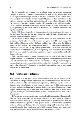

![Different users will require different things from an AM machine. Machines
vary in terms of cost, size, range of materials, accuracy of part, time of build, etc. It
is not surprising to know that the more expensive machines provide the wider range
of options and, therefore, it is important for someone looking to buy a new machine
to be able to understand the costs vs. the benefits so that it is possible to choose the
best machine to suit their needs.
Approaching a manufacturer or distributor of AM equipment is one way to get
information concerning the specification of their machine. Such companies are
obviously biased towards their own product and, therefore, it is going to be difficult
to obtain truly objective opinions. Conventions and exhibitions are a good way to
make comparisons, but it is not necessarily easy to identify the usability of
machines. Contacting existing users is sometimes difficult and time consuming,
but they can give very honest opinions. This approach works best if you are already
equipped with background information concerning your proposed use of the
technology.
When looking for advice about suitable selection methods or systems, it is useful
to consider the following points. One web-based system was developed to meet
these considerations [20]. An alternative approach will be presented in the next
section.
• The information in the system should be unbiased wherever possible.
• The method/system should provide support and advice rather than just a
quantified result.
• The method/system should provide an introduction to AM to equip the user with
background knowledge as well as advice on different AM technologies.
• A range of options should be given to the user in order to adjust requirements and
show how changes in requirements may affect the decision.
• The system should be linked to a comprehensive and up-to-date database of AM
machines.
• After the search process has completed, the system should give guidance on
where to look next for additional information.
The process of accessing the system should be as beneficial to the user as the
answers it gives. However, this is not as easy a task as one might first envisage. If it
were possible to decouple the attributes of the system from the user specification,
Table 13.3 Merit values
and rankings
Scenario 1 Scenario 2
Merit Rank Merit Rank
Proc 1 0.254 6 0.284 6
Proc 2 0.743 2 0.667 4
Proc 3 0.689 4 0.703 2
Proc 4 0.753 1 0.808 1
Proc 5 0.528 5 0.539 5
Proc 6 0.72 3 0.697 3
314 13 Guidelines for Process Selection](https://image.slidesharecdn.com/1-230308091212-68402451/85/1-Additive-manufacturing-pdf-330-320.jpg)
![then it would be a relatively simple task to select one machine against another. To
illustrate that this is not always possible, consider the following scenarios:
1. In a Powder Bed Fusion (PBF) machine, warm-up and cool down are important
stages during the build cycle that do not directly involve parts being fabricated.
This means that large parts do not take proportionally longer times to build
compared with smaller ones. Large builds are more efficient than small ones. In
Vat Photopolymerization (VP) and Material Extrusion (ME) machines, there is a
much stronger correlation between part size and build time. Small parts would
therefore take less time on a VP or ME machine than when using PBF, if
considered in isolation. Many users, however, batch process their builds and
the ability to vertically stack parts in a PBF machine makes it generally possible
to utilize the available space more efficiently. The warm-up and cool down
overheads are less important for larger builds and the time per layer is generally
quicker than most SL and ME machines. As a result of this discussion, it is not
easy to see which machine would be quicker without carefully analyzing the
entire process plan for using a new machine.
2. Generally, it costs less to buy a Dimension or other low-end ME machine
compared to a Binder Jetting (BJ) machine. There are technical differences
between these machines that make them suitable for different potential
applications. However, because they are in a similar price bracket, they are
often compared for similar applications. Dimension ME machines use a
cartridge-based material delivery system that requires a complete replacement
of the cartridge when empty. This makes material use much more expensive
when compared with the 3D Systems BJ (aka “ZCorp”) machine. For occasional
use, it is therefore perhaps better to use a Dimension machine when all factors
are equal. On the other hand, the more parts you build, the more cost-effective
the BJ machine becomes.
3. Identifying a new application or market can completely change the economics of
a machine. For example, in the metals area, directed energy deposition machines
(e.g., LENS, DMD) tend to be slower and have worse feature detail capability
than powder bed metal machines (e.g., SLM, EBM, DMLS). This has led to
many more machine sales for ARCAM, Renishaw, and EOS. However, some
companies identified a market for repairing molds and metal parts, which is very
difficult, if not impossible, with a powder bed machine.
These examples indicate that selection results depend to a large extent on the
user’s knowledge of AM capabilities and applications. Selection tools that include
expert systems may have an advantage over tools based on straightforward decision
methods alone. Expert systems attempt to embody the expertise resulting from
extensive use of AM technology into a software package that can assist the user in
overcoming at least some of the learning curve quickly and in a single stage. See
[20] for a more complete coverage of this idea.
13.3 Challenges of Selection 315](https://image.slidesharecdn.com/1-230308091212-68402451/85/1-Additive-manufacturing-pdf-331-320.jpg)
![13.4 Example System for Preliminary Selection
A preliminary selection tool was developed for AM, called AMSelect, that walks
the user through a series of questions to identify feasible processes and machines
[21]. Build times and costs are computed, but quantitative rating and rank-ordering
are not performed. More specifically, the software enables designers, managers, and
service bureau personnel to:
• Explore AM technologies for their application in a possible DDM project
• Identify candidate materials and processes
• Explore build times, build options, costs
• Explore manufacturing and life-cycle benefits of AM
• Select appropriate AM technologies for DDM applications
• Explore case studies, anticipate benefits
• Support Quotation and Capital Investment decisions
Figure 13.5 illustrates the logic underlying AMSelect. A database of machine
types and capabilities is read, which represents the set of machines that the software
will consider. The software supports a qualitative assessment of the suitability of
DDM for the application, then enables the user to explore the performance of
various AM machines. Build time and cost estimates are provided, which enable
the user to make a selection decision.
To use AMSelect, the user first enters information about the production project,
including production rate (parts per week), target part cost, how long the part is
expected to be in production, and the useful life of the part. After the user enters
Fig. 13.5 Flowchart of AMSelect operation
316 13 Guidelines for Process Selection](https://image.slidesharecdn.com/1-230308091212-68402451/85/1-Additive-manufacturing-pdf-332-320.jpg)
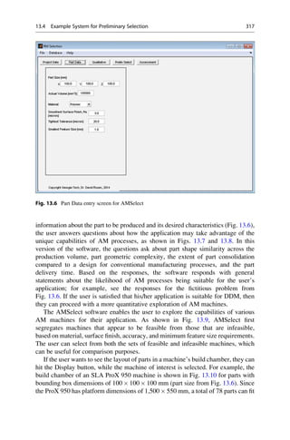
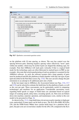
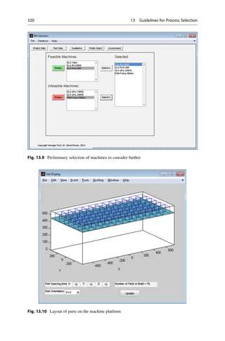
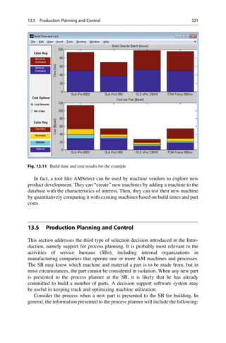
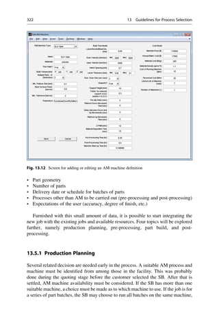
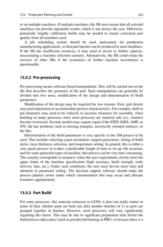
![significant delay between layers. In the latter case, it is obvious that the cumulative
number of layers should be as low as possible to minimize the overall build time for
many parts.
Another factor is part orientation. It is well known that because of anisotropic
properties caused by most AM processes, parts will generally build more effec-
tively in one orientation compared with another. This can cause difficulties when
organizing the batch production of parts. Orientation of parts so that they fit
efficiently within the work volume does not necessarily mean optimal build quality
and vice versa. For those machines that need to use support structures during the
build process, this represents an additional problem, both in terms of build time
(allocation of time to build the support structures for different orientations) and
post-processing time (removing the supports). Many researchers have discussed
these dilemmas [22].
What this generally means to a process planner is compromise. Compromise is
not unusual to a process planner; in fact, it is a typical characteristic, but the degree
of flexibility provided by many AM machines makes this a particularly interesting
problem. Just because an AM machine is being used constantly does not mean it is
being used efficiently.
13.5.4 Post-processing
All AM parts require a degree of post-processing. At the low end, this may require
removal of support structures or excess powder for those who merely want quick,
simple verification. At the high end, the AM process may be a very insignificant
time overhead in the overall process. Parts may require a large amount of skilled
manual work in terms of surface preparation and coating. Alternatively, the AM
part may be one stage in a complex rapid tooling process that requires numerous
manual and automated stages. All this can result from the same source machine. It
can even be an iterative process involving all of the above steps at different stages in
the development cycle based on the same part CAD data.
13.5.5 Summary
It is clear that only process planners who have a very detailed understanding of all
the roles that AM parts can play will be able to utilize the resources effectively and
efficiently. Even then it may be difficult to perform this task reliably given the large
number of variables involved. A software system to assist in this difficult task
would be a very valuable tool.
324 13 Guidelines for Process Selection](https://image.slidesharecdn.com/1-230308091212-68402451/85/1-Additive-manufacturing-pdf-340-320.jpg)


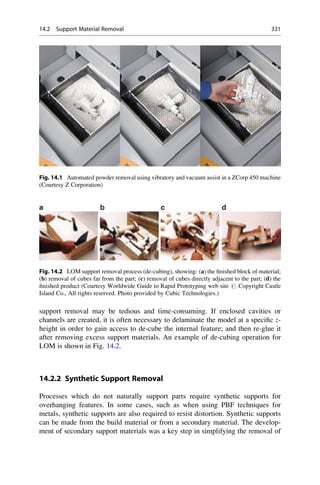
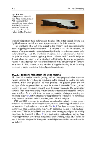
![14.2.2.2 Supports Made from Secondary Materials
A number of secondary support materials have been developed over the years in
order to alleviate the labor-intensive manual removal of support materials. Two of
the first technologies to use secondary support materials were the Cubital layer-
wise vat photopolymerization process and the Solidscape material jetting process.
Their use of wax support materials enabled the block of support/build to be placed
in a warm water bath; thus, melting or dissolving the wax yields the final parts.
Fig. 14.5 SLM dental
framework (# Emerald
Group Publishing Limited)
[1]
Fig. 14.4 Breakaway support removal for (a) an FDM part (courtesy of Jim Flowers) and (b) an
SLA part (Courtesy Worldwide Guide to Rapid Prototyping web site. # Copyright Castle Island
Co., All rights reserved. Photo provided by Cadem A.S., Turkey)
14.2 Support Material Removal 333](https://image.slidesharecdn.com/1-230308091212-68402451/85/1-Additive-manufacturing-pdf-348-320.jpg)
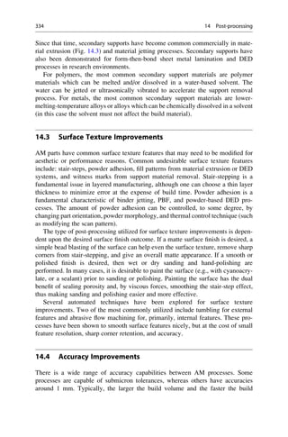
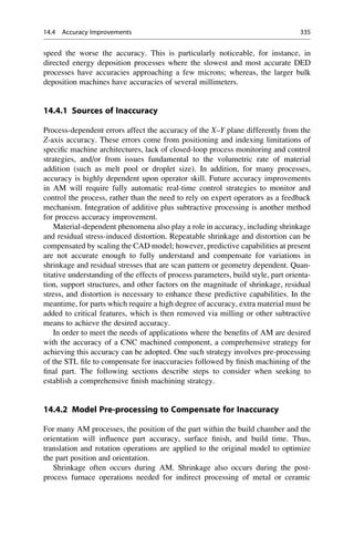
![green parts. Pre-process manipulation of the STL model will allow a scale factor to
be used to compensate for the average shrinkage of the process chain. However,
when compensating for average shrinkage, there will always be some features
which shrink slightly more or less than the average (shrinkage variation).
In order to compensate for shrinkage variation, if the highest shrinkage value is
used then ribs and similar features will always be at least as big as the desired
geometry. However, channels and holes will be too large. Thus, simply using the
largest shrinkage value is not an acceptable solution.
In order to make sure that there is enough material left on the surface to be
machined, adding “skin” to the original model is necessary. This skin addition, such
that there is material left to machine everywhere, can be referred to as making the
part “steel-safe.” Many studies have shown that shrinkage variations are geometry
dependent, even when using the same AM or furnace post-processing parameters.
Thus, compensating for shrinkage variation requires offsetting of the original model
to guarantee that even the features with the largest shrinkage levels and all channels
and holes are steel-safe.
There are two primary methods for adding a skin to the surface of a part. The first
is to offset the surfaces and then recalculate all of the surface intersections. This
methodology, though the most common, has many drawbacks for STL files made
up of triangular facets. In answer to these drawbacks, an algorithm developed for
offsetting all of the individual vertices of an STL file by using the normal vector
information for the connected triangles, then reconstructing the triangles by using
new vertex values, has been developed [2]. See Chap. 15 for more information on
STL files and software systems to manipulate them.
In an STL file, each vertex is typically shared by several triangles whose unit
normal vectors are different. When offsetting the vertices of a model, the new value
of each vertex is determined by the unit normal values of its connected triangles.
Suppose Voffset is the unit vector from the original position to the new position of
the vertex which is to be moved, and N1, N2, . . . Nn are the unit normal vectors of the
triangles which share that vertex; Voffset can be calculated by the weighted mean of
those unit normal vectors,
Voffset ¼
X
n
i¼1
WiNi ð14:1Þ
where Wi are coefficients whose values are determined to satisfy the equation,
Voffset N ¼ 1 i ¼ 1, 2, . . . n
ð Þ ð14:2Þ
After solving forVoffset;the new position Pnew of the vertex is given by the equation,
Pnew ¼ Porignal þ Voffset∗doffset ð14:3Þ
where doffset is the offset dimension set by the user.
336 14 Post-processing](https://image.slidesharecdn.com/1-230308091212-68402451/85/1-Additive-manufacturing-pdf-351-320.jpg)
![The above procedure is repeated until the new position values for all vertices are
calculated. The model is then reconstructed using the new triangle information.
Thus, to use this offset methodology, one need to only enter a doffset value that is
the same as the largest shrinkage variation anticipated. In practical terms, doffset
should be set equal to 2 or 3 times the absolute standard deviation of shrinkage
measured for a particular machine/material combination.
14.4.3 Machining Strategy
Machining strategy is very important for finishing AM parts and tools. Considering
both accuracy and machine efficiency, adaptive raster milling of the surface, plus
hole drilling and sharp edge contour machining can fulfill the needs of most parts.
14.4.3.1 Adaptive Raster Milling
When raster machining is used for milling operations, stepover distance between
adjacent toolpaths is a very important parameter that controls the machining
accuracy and surface quality. It is known that higher accuracy and surface quality
require a smaller stepover distance. Normally, the cusp height of material left after
the model is machined is used as a measurement of the surface quality.
Figure 14.6 shows a triangle face being machined with a ball endmill. The
relationship between cusp height h, cutter radius r, stepover distance d, and incline
angle α is given in the following equation:
d ¼ 2:0
ffiffiffiffiffiffiffiffiffiffiffiffiffiffiffiffiffiffiffiffiffiffiffiffiffiffi
r2 r h
ð Þ2
q
cos α ð14:4Þ
α is determined by the triangle surface normal and stepover direction. Suppose
Ntriangle is the unit normal vector of the triangle surface, and NStepover is the unit
vector along stepover direction, then
α
d
r
h
l
Fig. 14.6 Illustration for
determining stepover distance
(# Emerald Group
Publishing Limited) [3]
14.4 Accuracy Improvements 337](https://image.slidesharecdn.com/1-230308091212-68402451/85/1-Additive-manufacturing-pdf-352-320.jpg)
![cos
π
2
α
¼ sin α ¼ NTriangle NStepover
ð14:5Þ
From (14.4) and (14.5), the following equation for stepover distance is derived,
d ¼ 2:0
ffiffiffiffiffiffiffiffiffiffiffiffiffiffiffiffiffiffiffiffiffiffiffiffiffiffiffiffiffiffiffiffiffiffiffiffiffiffiffiffiffiffiffiffiffiffiffiffiffiffiffiffiffiffiffiffiffiffiffiffiffiffiffiffiffiffiffiffiffiffiffiffiffiffi
h 2r h
ð Þ 1 NTriangle NStepover
2
r
ð14:6Þ
When machining the model, the cutter radius and milling direction are the same for
all triangle surfaces. If given the user-set maximum cusp height h, d is only related
to the triangle normal vector. For surfaces with different normal vectors, the
stepover distance obtained will be different.
If using a constant stepover distance, in order to guarantee a particular machin-
ing tolerance, the minimum calculated d should be used for the entire part. How-
ever, using the minimum stepover distances will lead to longer programs and
machining times. Therefore, an adaptive stepover distance for milling operations
according to local geometry should be used to allow for both accuracy and machine
efficiency. This means that stepover distances are calculated dynamically for each
just-finished tool pass, using the maximum cusp height to determine the stepover
distance for the next tool pass.
An example of the use of this type of algorithm for tool-path generation is shown
in Fig. 14.7. As can be seen, for tool paths which pass through a region of high
angle, the tools paths are more closely spaced; whereas, for toolpaths that only cross
relatively flat regions, the tool paths are widely spaced.
14.4.3.2 Sharp Edge Contour Machining
Sharp edges are often the intersection curves between features and surfaces.
Normally, these edges define the critical dimensions. When using raster milling,
the edges parallel to the milling direction can be missed, causing large errors. As
shown in Fig. 14.8, when a stepover distance d is used to machine a part with slot
width W, even when the CNC machine is perfectly aligned (i.e., ignoring machine
positioning errors), the slot width error will be at least,
Werror ¼ 2d δ1 δ2 ð14:6Þ
where δ1, δ2 represent the offset between the actual and desired edge location.
When δ1, δ2 become 0, Werror ¼ 2d. This means that the possible maximum error
for a slot using raster milling is approximately two times the stepover distance.
For complicated edges not parallel to the milling direction, raster milling is
ineffective for creating smooth edges, as the edge will have a stair-step appearance,
with the step size equal to the local stepover distance, d. Thus, after raster milling, it
is advantageous to run a machining pass along the sharp edges (contours) of the part
[3]. In order to machine along sharp edges, all sharp edges must first be identified
from the STL model. The normal vector information of each triangle is used to
check the property of an edge. The angle between normal vectors of two
338 14 Post-processing](https://image.slidesharecdn.com/1-230308091212-68402451/85/1-Additive-manufacturing-pdf-353-320.jpg)
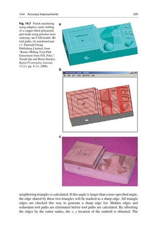
![z value is determined by calculating the intersection with the 3D model and finding
the corresponding maximum z value. Using this approach, sharp edges can be
identified and easily finish machined. Figure 14.9 shows the part from Fig. 14.7
with sharp edge contour paths highlighted.
14.4.3.3 Hole Drilling
Circular holes are common features in parts and tools. Using milling tools to create
holes is inefficient and the circularity of the holes is poor. Therefore, a machining
strategy of identifying and drilling holes is preferable. The most challenging aspect
is to recognize holes in an STL or AMF file, as the 3D geometry is represented by a
collection of unordered triangular planar facets (and thus all feature information
is lost).
The intersection curve between a hole and a surface is typically a closed loop. By
using this information, a hole recognition algorithm begins by identifying all closed
Fig. 14.8 Influence of
stepover distance on
dimensional accuracy (#
Emerald Group Publishing
Limited) [3]
Fig. 14.9 Sharp edge contours identified for milling
340 14 Post-processing](https://image.slidesharecdn.com/1-230308091212-68402451/85/1-Additive-manufacturing-pdf-355-320.jpg)
![loops made up of sharp edges from the model. These closed loops may not
necessarily be the intersection curves between holes and a surface, so a series of
hole-checking rules are used to remove the loops that do not correspond to drilled
holes. The remaining loops and their surface normal vectors are used to determine
the diameter, axis orientation, and depth for drilling. From this information, tool
paths can be automatically generated [3].
Thus, by pre-processing an STL file using a shrinkage and surface offset value,
and then post-processing the part using adaptive raster milling, contour machining,
and hole drilling, an accurate part can be made. In many cases, however, this type of
comprehensive strategy is not necessary. For instance, for a complex part where
only one or two features must be made accurately, the part could be pre-processed
using the average shrinkage value as a scaling factor and a skin can be added only to
the critical features. These critical features could then be manually machined after
AM part creation, leaving the other features as is. Thus, the finish machining
strategy adopted will depend greatly upon the application and part-specific design
requirements.
14.5 Aesthetic Improvements
Many times AM is used to make parts which will be displayed for aesthetic or
artistic reasons or used as marketing tools. In these and similar instances, the
aesthetics of the part is of critical importance for its end application.
Often the desired aesthetic improvement is solely related to surface finish. In this
case, the post-processing options discussed in Sect. 14.2 can be used. In some cases,
a difference in surface texture between one region and another may be desired (this
is often the case in jewelry). In this case, finishing of selected surfaces only is
required (such as for the cover art for this book).
In cases where the color of the AM part is not of sufficient quality, several
methods can be used to improve the part aesthetics. Some types of AM parts can be
effectively colored by simply dipping the part into a dye of the appropriate color.
This method is particularly effective for parts created from powder beds, as the
inherent porosity in these parts leads to effective absorption. If painting is required,
the part may need to be sealed prior to painting. Common automotive paints are
quite effective in these instances.
Another aesthetic enhancement (which also strengthens the part and improves
wear resistance) is chrome plating. Figure 14.10 shows a stereolithography part
before and after chrome plating. Several materials have been electroless coated to
AM parts, including Ni, Cu, and other coatings. In some cases, these coatings are
thick enough that, in addition to aesthetic improvements, the parts are robust
enough to use as tools for injection molding or as EDM electrodes.
14.5 Aesthetic Improvements 341](https://image.slidesharecdn.com/1-230308091212-68402451/85/1-Additive-manufacturing-pdf-356-320.jpg)

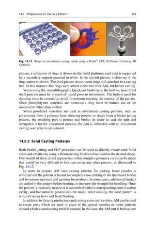
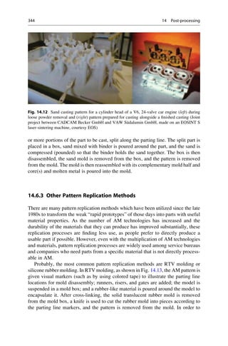
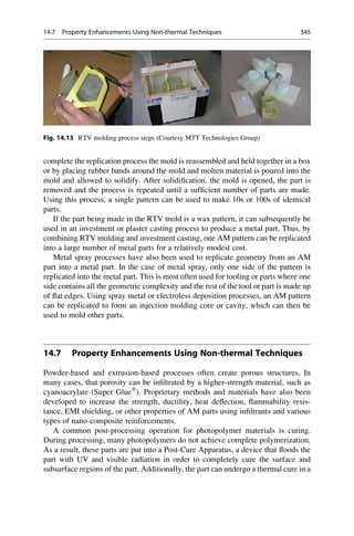
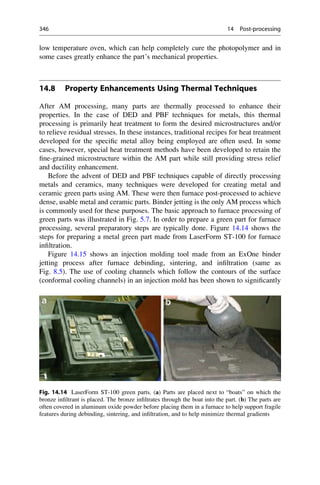
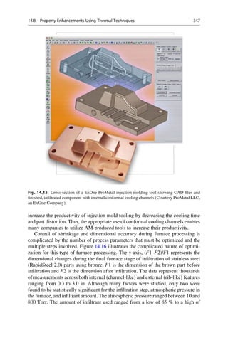
![110 %, where the percentage amount was based upon the theoretical amount of
material needed to fully fill all of the porosity in the part, based upon measurements
of the weight and the volume of the part just prior to infiltration.
It can be seen from Fig. 14.16 that the factor combinations with the lowest
overall shrinkage were not the factors with the lowest shrinkage variation. Factor
combination A had the lowest average shrinkage, while factor combination E had
the lowest shrinkage variation. As average shrinkage can be easily compensated
using a scaling factor, the optimum factor combination for highest accuracy and
precision would be factor combination E. If the accuracy strategy discussed in
Sect. 14.3 is followed, the skin offset doffset would be determined by identifying the
shrinkage variation for the entire process (green part fabrication using AM, plus
sintering and infiltration) using a similar approach and then setting doffset equal to
the maximum shrinkage variation at the desired confidence interval.
In addition to the thermal processes discussed earlier, a number of other
procedures have been developed over the years to combine AM with furnace
processing to produce metal or ceramic parts. One example approach utilized laser
sintering to produce porous parts with gas impermeable skins. By scanning only the
outside contours of a part during fabrication by SLS, a metal “can” filled with loose
powder is made. These parts are then post-processed to full density using hot
isostatic pressing (HIP). This in situ encapsulation results in no adverse container–
powder interactions (as they are made from the same bed of powder), reduced
pre-processing time, and fewer post-processing steps compared to conventional
HIP of canned parts. The SLS/HIP approach was successfully used to produce
complex 3D parts in Inconel 625 and Ti–6Al–4 V for aerospace applications [4].
Laser sintering has also been used to produce complex-shaped ZrB2/Cu com-
posite EDM electrodes. The approach involved (a) fabrication of a green part from
polymer coated ZrB2 powder using the laser sintering, (b) debinding and sintering
of the ZrB2, and (c) infiltration of the sintered, porous ZrB2 with liquid copper. This
manufacturing route was found to result in a more homogeneous structure com-
pared to a hot pressing route.
Fig. 14.16 Ninety-five
percent confidence intervals
for variation in shrinkage for
stainless steel (RapidSteel
2.0) infiltration by bronze
(Factor combinations are: (a)
10 Torr, 80 %; (b) 10 Torr,
95 %; (c) 10 Torr, 110 %; (d)
800 Torr, 80 %; (e) 800 Torr,
95 %; (f) 800 Torr, 110 %)
348 14 Post-processing](https://image.slidesharecdn.com/1-230308091212-68402451/85/1-Additive-manufacturing-pdf-363-320.jpg)

![This chapter will describe the fundamentals for creating output files for AM. It
will discuss the most common technique, which is to create the STL file format,
explaining how it works and typical problems associated with it. Some of the
numerous software tools for use with AM will be described and possible effects
of new concepts in AM on the development of associated software tools in the
future will be discussed. Finally, there will be a discussion concerning the Additive
Manufacturing File (AMF) format, which has been developed to address the needs
of future AM technology where more than just the geometric information may be
required.
15.2 Preparation of CAD Models: The STL File
The STL file is derived from the word STereoLithography, which was the first
commercial AM process, produced by the US company 3D Systems in the late
1980s [1], although some have suggested that STL should stand for
Stereolithography Tessellation Language. STL files are generated from 3D CAD
data within the CAD system. The output is a boundary representation that is
approximated by a mesh of triangles.
15.2.1 STL File Format, Binary/ASCII
STL files can be output as either binary or ASCII (text) format. The ASCII format is
less common (due to the larger file sizes) but easier to understand and is generally
used for illustration and teaching. Most AM systems run on PCs using Windows.
The STL file is normally labeled with a “.STL” extension that is case insensitive,
although some AM systems may require a different or more specific file definition.
These files only show approximations of the surface or solid entities and so any
information concerning the color, material, build layers, or history is ignored during
the conversion process. Furthermore, any points, lines, or curves used during the
construction of the surface or solid, and not explicitly used in that solid or surface,
will also be ignored.
An STL file consists of lists of triangular facets. Each triangular facet is uniquely
identified by a unit normal vector and three vertices or corners. The unit normal
vector is a line that is perpendicular to the triangle and has a length equal to 1.0.
This unit length could be in mm or inches and is stored using three numbers,
corresponding to its vector coordinates. The STL file itself holds no dimensions,
so the AM machine operator must know whether the dimensions are mm, inches, or
some other unit. Since each vertex also has three numbers, there are a total of
12 numbers to describe each triangle. The following file shows a simple ASCII STL
file that describes a right-angled, triangular pyramid structure, as shown in
Fig. 15.1.
Note that the file begins with an object name delimited as a solid. Triangles can
be in any order, each delimited as a facet. The facet line also includes the normal
352 15 Software Issues for Additive Manufacturing](https://image.slidesharecdn.com/1-230308091212-68402451/85/1-Additive-manufacturing-pdf-367-320.jpg)
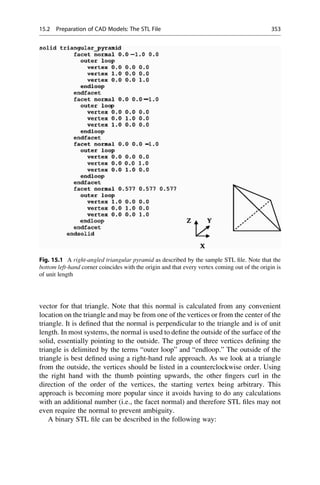
![– An 80-byte ASCII header that can be used to describe the part
– A 4 byte unsigned long integer that indicates the number of facets in the object
– A list of facet records, each 50 bytes long
The facet record will be presented in the following way:
– 3 floating values of 4 bytes each to describe the normal vector
– 3 floating values of 4 bytes each to describe the first vertex
– 3 floating values of 4 bytes each to describe the second vertex
– 3 floating values of 4 bytes each to describe the third vertex
– One unsigned integer of 2 bytes, that should be zero, used for checking
15.2.2 Creating STL Files from a CAD System
Nearly all geometric solid modeling CAD systems can generate STL files from a
valid, fully enclosed solid model. Most CAD systems can quickly tell the user if a
model is not a solid. This test is particularly necessary for systems that use surface
modeling techniques, where it can be possible to create an object that is not fully
closed off. Such systems would be used for graphics applications where there is a
need for powerful manipulation of surface detail (like with Autodesk AliasStudio
software [2] or Rhino from Robert McNeel Associates [3]) rather than for
engineering detailing. Solid modeling systems, like SolidWorks, may use surface
modeling as part of the construction process, but the final result is always a solid
that would not require such a test.
Most CAD systems use a “Save as” or “Export” function to convert the native
format into an STL file. There is typically some control over the size of the triangles
to be used in the model. Since STL uses planar surfaces to approximate curved
surfaces, then obviously the larger the triangles, the looser that approximation
becomes. Most CAD systems do not directly limit the size of the triangles since it
is also obvious that the smaller the triangle, the larger the resulting file for a given
object. An effective approach would be to minimize the offset between the triangle
and the surface that it is supposed to represent. A perfect cube with perfectly sharp
edges and points can be represented by 12 triangles, all with an offset of 0 between
the STL file and the original CAD model. However, few designs would be that
convenient and it is important to ensure a good balance between surface approxi-
mation and excessively large file. Figure 15.2 shows the effect of changing the
triangle offset parameter on an STL file. The exact value of the required offset
would largely depend on the resolution or accuracy of the AM process to be used. If
the offset is smaller than the basic resolution of the process, then making it smaller
will have no effect on the precision of the resulting model. Since many AM
processes operate around the 0.1 mm layer resolution, then a triangle offset of
0.05 mm or slightly lower will be acceptable for fabrication of most parts.
354 15 Software Issues for Additive Manufacturing](https://image.slidesharecdn.com/1-230308091212-68402451/85/1-Additive-manufacturing-pdf-369-320.jpg)
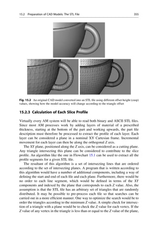
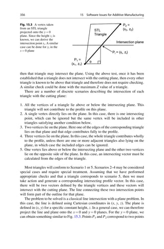
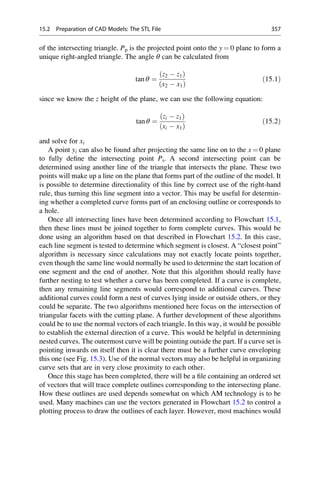
![also need to fill in these outlines to make a solid. Flowchart 15.3 uses an inside/
outside algorithm to determine when to switch on a filling mechanism to draw
scanning lines perpendicular to one of the planar axes. The assumption is that the
part is fully enclosed inside the build envelope and therefore the default fill is
switched off.
Start
Read in STL
Extract facet
data from STL
Scan facet data
Get vertices
no yes
All facets
scanned?
yes
no
Finish
Compare facet
with cutting
plane
Intersection?
Store
intersection line
of facet on plane
Flowchart 15.1 Algorithm for testing triangles and generating line intersections. The result will
be an unordered matrix of intersecting lines (adapted from [4])
358 15 Software Issues for Additive Manufacturing](https://image.slidesharecdn.com/1-230308091212-68402451/85/1-Additive-manufacturing-pdf-373-320.jpg)
![15.2.4 Technology-Specific Elements
Flowcharts 15.1, 15.2, and 15.3 are basic algorithms that are generic in nature.
These algorithms need to be refined to prevent errors and to tailor them to suit a
particular process. Other refinements may be employed to speed the slicing process
up by eliminating redundancy, for example.
As mentioned in previous chapters, many AM systems require parts built using
support structures. Supports are normally a loose-woven lattice pattern of material
placed below the region to be supported. Such a lattice pattern could be a simple
Start
Select a line
and store in
new line matrix
Measure
distance
between tail of
line and all
other lines
Have all lines
been checked?
Find minimum
distance and
its related line
Swap head and
tail of related
line
no
yes
Finish
yes
no
Does minimum
distance relate to head of
related line?
Store this line
in order in new
line matrix
Flowchart 15.2 Algorithm for ordering the line intersections into complete outlines. This
assumes there is only a single contour in each plane (adapted from [4])
15.2 Preparation of CAD Models: The STL File 359](https://image.slidesharecdn.com/1-230308091212-68402451/85/1-Additive-manufacturing-pdf-374-320.jpg)
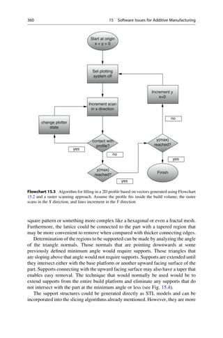
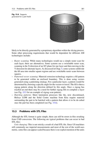
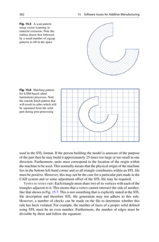
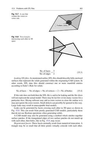
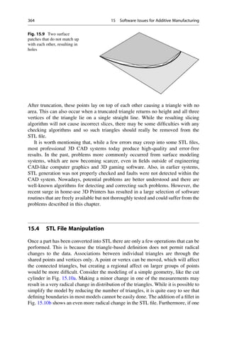
![were to attempt to move the oval that represents the cut surface, the triangles
representing the filet would no longer show a constant-radius curve.
Building models using AM is often done by people working in departments or
companies that are separate from the original designers. It may be that whoever is
building the model may not have direct access to the original CAD data. There may
therefore be a need to modify the STL data before the part is to be built. The
following sections discuss STL tools that are commonly used.
15.4.1 Viewers
There are a number of STL viewers available, often as a free download. An example
is STLview from Marcam [5] (see Fig. 15.11). Like many other systems, this
software allows limited access to the STL file, making it possible to view the
triangles, apply shading, show sections, etc. By purchasing the full software
version, other tools are possible, for example, allowing the user to measure the
part at various locations, annotate the part, display slice information, and detect
potential problems with the data. Often the free tools allow passive viewing of the
STL data, while the more advanced tools permit modification of the data, either by
rewriting the STL or supplying additional information with the STL data (like
measurement information, for example). Often these viewers are connected to part
building services and provided by the company as an incentive to use these services
and to help reduce errors in data transfer, either from incorrect STL conversion or
from wrong interpretation of the design intent.
15.4.2 STL Manipulation on the AM Machine
STL data for a part consist of a set of points defined in space, based on an arbitrarily
selected point of origin. This origin point may not be appropriate to the machine the
part is to be built on. Furthermore, even if the part is correctly defined within the
machine space, the user may wish to move the part to some other location or to
Fig. 15.10 STL files of a cut cylinder. Note that although the two models in (a) are very similar,
the location of the triangles is very different. Addition of a simple filet in (b) shows even greater
change in the STL file
15.4 STL File Manipulation 365](https://image.slidesharecdn.com/1-230308091212-68402451/85/1-Additive-manufacturing-pdf-380-320.jpg)
![make a duplicate to be built beside the original part. Other tasks, like scaling,
changing orientation, and merging with other STL files are all things that are
routinely done using the STL manipulation tools on the AM machine.
Creation of the support structures is also something that would normally be
expected to be done on the AM machine. This would normally be done automati-
cally and would be an operation applied to downward-facing triangles. Supports
would be extended to the base of the AM machine or to any upward facing triangle
placed directly below. Triangles that are only just veering away from the vertical
(e.g., less than 10
) may be ignored for some AM technologies. Note, for example,
the supports generated around the cup handle in Fig. 15.4.
With some AM operating systems there is little or no control over placement of
supports or manipulation of the model STL data. Considering Fig. 15.4 again, it
may be possible to build the handle feature without so many supports, or even with
no supports at all. A small amount of sagging around the handle may be evident, but
the user may prefer this to having to clean up the model to remove the support
material. If this kind of control is required by the user, it may be necessary to
purchase additional third party software, like the MAGICS and 3-matic systems
from Materialise [6].
Such third party software may also be used to undertake additional roles.
MAGICS, for example, has a number of modules useful to many AM technologies.
Other STL file manipulators may have similar modules:
– Checking the integrity of STL files based on the problems described above.
– Incorporating support structures including tapered features on the supports that
may make them easier to remove.
– Optimizing the use of AM machines, like ensuring the machine is efficiently
filled with parts, the amount of support structures is minimized, etc.
Fig. 15.11 The VisCAM viewer from Marcam that can be used to inspect STL models
366 15 Software Issues for Additive Manufacturing](https://image.slidesharecdn.com/1-230308091212-68402451/85/1-Additive-manufacturing-pdf-381-320.jpg)
![– Adding in features like serial numbers and identifying marks onto the parts to
ensure correct identification, easy assembly, etc.
– Remeshing STL files that may have been created using Reverse Engineering
software or other non-CAD-based systems. Such files may be excessively large
and can often be reduced in size without compromising the part accuracy.
– Segmenting large models or combining multiple STL files into a single model
data set.
– Performing Boolean tasks like subtracting model data from a tool insert blank
model to create a mold.
15.5 Beyond the STL File
The STL definition was created by 3D Systems right at the start of the development
history of AM technology and has served the industry well. However, there are
other ways in which files can be defined for creation of the slice. Furthermore, the
fact that the STL file only represents the surface geometry may cause problems for
parts that require some heterogeneous content. This section will discuss some of the
issues surrounding this area.
15.5.1 Direct Slicing of the CAD Model
Since generation of STL files can be tedious and error-prone, there may be some
benefit from using inbuilt CAD tools to directly generate slice data for the AM
machines. It is a trivial task for most 3D solid modeling CAD systems to calculate
the intersection of a plane with a model, thus extracting a slice. This slice data
would ordinarily need to be processed to suit the drive system of the AM technol-
ogy, but this can be handled in most CAD systems with the use of macros. Support
structures can be generated using standard geometry specifications and projected
onto the part from a virtual representation of the AM machine build platform.
Although this approach has never been a popular method for creating slice data,
it has been investigated as a research topic [7] and even developed to suit a
commercialized variant of the Stereolithography process by a German company
called Fockle Schwarz. The major barrier to using this approach is that every
CAD system must include a suite of different algorithms for direct slicing for a
variety of machines or technologies. This would be a cumbersome approach that
may require periodic updates of the technology as new machines become available.
There may be some benefit in the future in creating an integrated design and
manufacturing solution, especially for niche applications or for low-cost solutions.
However, at present it is more sensible to separate the development of the design
tools from that of the AM technology by using the STL format.
15.5 Beyond the STL File 367](https://image.slidesharecdn.com/1-230308091212-68402451/85/1-Additive-manufacturing-pdf-382-320.jpg)
![15.5.2 Color Models
Currently, several AM technologies are available on the market that can produce
parts with color variations, including full color output, including the color binder
jetting technology from 3D Systems, material jetting machines from 3D Systems
and Stratasys, and sheet lamination systems from Mcor Technologies. Colored
parts have proven to be very popular, and it is likely that other color AM machines
will make their way to the market. The conventional STL file contains no informa-
tion pertaining to the color of the part or any features thereon. Coloring of STL files
is possible and there are in fact color STL file definitions available [8], but you
would be limited by the fact that a single triangle can only be one specific color. It is
therefore much better to use the VRML painting options that allow you to assign
bitmap images to individual facets [8]. In such a way, it is possible to take
advantage of the color possibilities that the AM machine can give you.
15.5.3 Multiple Materials
Carrying on from the previous section, color is one of the simplest examples of
multiple material products that AM is capable of producing. As has been mentioned
in other chapters, parts can be made using AM from composite materials, with
varying levels of porosity or indeed with regions containing discretely different
materials. For many of these new AM technologies, STL is starting to become an
impediment. Since the STL definition is for surface data only, the assumption
therefore is that the solid material between these surfaces is homogeneous. As we
can see from the above this may not be the case. While there has been significant
thought applied to the problem of representations for heterogeneous solid modeling
[9], there is still much to be considered before we can arrive at a standard to
supersede STL for future AM technology, as discussed in Sect. 15.7.
15.5.4 Use of STL for Machining
STL is used for applications beyond just converting CAD to additive manufacturing
input. Reverse Engineering packages can also be used to convert point cloud data
directly into STL files without the need for CAD. Such technology connected
directly to AM could conceivably form the basis for a 3D Fax machine. Another
technology that can easily make use of STL files is subtractive manufacturing.
Subtractive manufacturing systems can readily make use of the surface data
represented in STL to determine the boundaries for machining. With some addi-
tional knowledge concerning the dimensions of the starting block of material, tool,
machining center, etc., it is possible to calculate machining strategies for creating a
3D surface model. As mentioned in earlier chapters, the likelihood is that it may not
be possible to fully machine complex geometries due to undercutting features,
internal features, etc. but there is no reason why STL files cannot be used to create
368 15 Software Issues for Additive Manufacturing](https://image.slidesharecdn.com/1-230308091212-68402451/85/1-Additive-manufacturing-pdf-383-320.jpg)
![Computer Aided Manufacturing (CAM) profiles for machining centers. Delft
Spline [10] has been using STL files to create CAM profiles for a number of
years now. Figure 15.12 shows the progression of a model through to a tool to
manufacture a final product using their DeskProto software. Another technology
that uses a hybrid of subtractive and additive processes to fabricate parts is the SRP
(Subtractive Rapid Prototyping) technique developed by Roland [11] for their
desktop milling machines. The creation of finish machining tool paths for AM
parts from STL files is also discussed in Chap. 14.
15.6 Additional Software to Assist AM
As well as directly controlling the manufacturing process, other software systems
may be helpful in running an effective and efficient AM-based facility.
Fig. 15.12 DeskProto software being used to derive machine tool paths from STL file data to
form a mold for creating the windscreen of a motorcycle
15.6 Additional Software to Assist AM 369](https://image.slidesharecdn.com/1-230308091212-68402451/85/1-Additive-manufacturing-pdf-384-320.jpg)
![15.6.1 Survey of Software Functions
Such software can include one or more of the following functions:
Simulation: Many operating systems can perform a simulation of the machines
operations in a build process, showing how the layers will be formed step by step in
accelerated time. This can allow the user to detect obvious errors in the slice files
and determine whether critical features can be built. This may be particularly
important for processes like material extrusion where the hatch patterns can have
a critical effect on thin wall features, for example. Some work has been carried out
to simulate AM systems to get a better impression of the final result, including
rendered images to give an understanding of the surface roughness for a given layer
thickness, for example [12].
Build-time estimation: AM is a highly automated process and the latest machines
are very reliable and can operate unattended for long periods of time. For effective
process planning it is very important to know when a build is going to be completed.
Knowing this will help in determining when operators will be required to change
over jobs. Good estimates will also help to balance builds; adding or subtracting a
part from the job batch may ensure that the machine cycle will complete within a
day-shift, for example, making it possible to keep machines running unattended at
night. Also, if you are running multiple machines, it would be helpful to stagger the
builds throughout the shift to optimize the manual work required. Early build-time
estimation software was extremely unreliable, performing rolling calculations of
the average build time per layer. Since the layer time is dependent on the part
geometry, such estimates could be very imprecise and vary wildly, especially at the
beginning of a build. Later software versions saw the benefit in having more precise
build-time estimations. A simplified build-time model is discussed in Chap. 16.
Machine setup: While every AM machine has an operating system that makes it
possible to set up a build, such systems can be very basic, particularly in terms of
manipulation of the STL files. Determining build parameters based on a specific
material is normally very comprehensive however.
Monitoring: This is a relatively new feature for most AM systems. Even though
nearly every AM machine will be connected either directly or indirectly to the
Internet, this has traditionally been for uploading of model files for building. Export
of information from the machine to the Internet or within an Intranet has not been
common except in the larger, more expensive machines. The simplest monitoring
systems would provide basic information concerning the status of the build and how
much longer before it is complete. However, more complex systems may tell you
about how much material is remaining, the current status parameters like
temperatures, laser powers, etc. and whether there is any need for manual interven-
tion through an alerting system. Some monitoring systems may also provide video
feedback of the build.
Planning: Having a simulation of the AM process running on a separate com-
puter may be helpful to those working in process planning. Process planners may be
able to determine what a build could look like, thus allowing the possibility of
planning for new jobs, variability analysis, or quoting.
370 15 Software Issues for Additive Manufacturing](https://image.slidesharecdn.com/1-230308091212-68402451/85/1-Additive-manufacturing-pdf-385-320.jpg)
![Once again such software may be available from the AM system vendor or from
a third party vendor. The advantage of third party software is that it is more likely to
be modified to suit the exact requirements of the user.
15.6.2 AM Process Simulations Using Finite Element Analysis
Finite element analysis (FEA) techniques are increasingly popular tools to predict
how the outcome of various manufacturing processes change with changing process
parameters, geometry and/or material. Commercial software packages such as
SYSWELD, COMSOL, MoldFlow, ANSYS, and DEFORM are used to predict
the outcomes of welding, forming, molding, casting, and other processes.
AM technologies are particularly difficult to simulate using predictive finite
element tools. For instance, the multiscale nature of metal powder bed fusion
approaches such as metal laser sintering and electron beam melting are incredibly
time consuming to accurately simulate using physics-based FEA. AM processes are
inherently multiscale in nature, and fine-scale finite element meshes that are 10 μm
or smaller in size are required to accurately capture the solidification physics
around the melt pool, while the overall part size can be 10,000 times larger than
the element size. In three dimensions, this means that if we apply a uniform 10 μm
mesh size, we would need 108
elements in the first layer and more than 1012
elements in total to capture the physics for a single part that fills much of a powder
bed. Since rapid movement of a point heat source is used to create parts, capturing
the physics requires a time step of 10 ms or less during laser/electron beam melting,
which for a complete build would require more than 1010
total time steps. To solve a
problem with this, number of elements for this many time steps on a relatively high-
speed supercomputer would take billions of years. Thus, to date all AM simulation
tools are limited to predictions of only a small fraction of a part, or very small,
simplified geometries.
Using existing FEA tools, several researchers are looking for ways to make
assumptions whereby they can cut and paste solutions from simplified geometries to
form a solution for large, complex geometries. This approach has the benefit of
faster solution time; however, for large, complex geometries these types of
predictions fail to accurately capture the effects of changing scan patterns, complex
accumulation of residual stresses, and localized thermal characteristics. In addition,
minor changes to input conditions can make the simplified solutions invalid. Thus a
simulation infrastructure which can quickly build up a “new” answer for any
arbitrary geometry, input condition, and scan pattern is the ultimate goal for a
predictive AM simulation tool.
Recently, researchers have begun using dynamic, multiscale moving meshes to
accelerate FEA analysis for AM [13]. These types of multiscale simulations are
many orders of magnitude faster than standard FEA simulations. However
multiscale simulations alone are still too slow to enable a complete part simulation,
even on the world’s fastest supercomputers. Thus a new computational approach
for AM is needed, which can extend FEA beyond its historical capabilities. 3DSIM,
15.6 Additional Software to Assist AM 371](https://image.slidesharecdn.com/1-230308091212-68402451/85/1-Additive-manufacturing-pdf-386-320.jpg)
![a new software start-up, is seeking to do that for the AM industry. 3DSIM software
tools include: (1) a new approach to formulating and solving multiscale moving
meshes, (2) a novel finite element-based Eigensolver which predicts thermal evo-
lution and residual stresses very quickly in regions of low thermal gradients, (3) an
insignificant number truncation Cholesky module which eliminates the “multipli-
cation by zero” calculations that occur when solving sparse finite element matrices,
and (4) an Eigenmodal approach to identifying periodicity in AM computations to
enable feed-forward “insertion” of solutions into regions where periodicity is
present and the solution is already known from a prior time step. These approaches
are reported to reduce the solution time for large-scale AM problems by orders of
magnitude. Taken together, these tools should make the full part problem solvable
in less than a day on a desktop GPU-based supercomputer when the algorithms are
fully implemented in a combined software infrastructure. If realized, the ability to
predict how process parameter and material changes affect part accuracy, distor-
tion, residual stress, microstructure, and properties would be a significant advance-
ment for the AM industry.
15.7 The Additive Manufacturing File Format
It has already been discussed that, while effective, there are numerous difficulties
surrounding the STL format. As AM technologies move forward to include multi-
ple materials, lattice structures, and textured surfaces, it is likely that an alternative
format will be required. The ASTM Committee F42 on Additive Manufacturing
Technologies released the ASTM 2915-12 AMF Standard Specification for AMF
Format 1.1 in May 2011 [14]. This file format is still very much under development,
but has already been implemented in some commercial and beta-stage software.
Considerably more complex than the STL format, AMF aims to embrace a whole
host of new part descriptions that have hindered the development of current AM
technologies. These include the following features:
Curved triangles: In STL, the surface normal lies on the same plane as the
triangle vertices that it is connected to. However, in AMF, the start location of the
normal vector does not have to lie on the same plane. If so, the corresponding
triangle must be curved. The definition of curvature is such that all triangle edges
meeting at that vertex are curved so that they are perpendicular to that normal and in
the plane defined by the normal and the original straight edge (i.e., if the original
triangle had straight edges rather than curved ones). By specifying the triangles in
this way, many fewer triangles need be used for a typical CAD model. This
addresses problems associated with large STL files resulting from complex geome-
try models for high-resolution systems. The curved triangle approach is still an
approximation since the degree of curvature cannot be too high. Overall accuracy is
however significantly improved in terms of cusp height deviation.
Color: Color can be assigned in a nested way so that the main body of the part
can be colored according to a function within the original design. Red, Green, and
Blue coloration can be applied along with a transparency value to vertices,
372 15 Software Issues for Additive Manufacturing](https://image.slidesharecdn.com/1-230308091212-68402451/85/1-Additive-manufacturing-pdf-387-320.jpg)
![3. Write out an ASCII STL file for a perfect cube, aligned with the Cartesian
coordinate frame, starting at (0, 0, 0) and all dimensions positive. Model the
same cube in a CAD system. Does it make the same STL file? What happens
when you make slight changes to the CAD design?
4. Why might it be possible that a part could inadvertently be built 25 times too
small or too large in any one direction?
5. Is it okay to ignore the vertex of a triangle that lies directly on an intersecting
cutting plane?
6. Prove to yourself with some simple examples that the number of faces divided
by the number of edges is 2/3.
7. Using the Wikipedia description of AMF [15] consider how you would code an
airplane wing model that has honeycomb internal lattice for lightweight and
some colored decorations on the outer skin. How might the part look using a
color ZPrinter compared to using an SL machine. What design considerations
would you still have to make to ensure the part is properly made on these
machines?
References
1. 3D Systems Inc (1989) Stereolithography interface specification. October 1989
2. Autodesk CAD software. usa.autodesk.com
3. Rhinoceros CAD software. http://www.rhino3d.com/
4. Vatani M, Rahimi AR et al (2009) An enhanced slicing algorithm using nearest distance
analysis for layer manufacturing. Proceedings of World Academy of Science, Engineering and
Technology, vol 37, pp 721–726, Jan 2009. ISSN: 2070-3740
5. Marcam, VisCAM software. http://www.marcam.de
6. Materialise, AM software systems. http://www.materialise.com/materialise/view/en/92074-
Magics.html
7. Jamieson R, Hacker H (1995) Direct slicing of CAD models for rapid prototyping. Rapid
Prototyping J 1(2):4–12, Pub. by Emerald, ISSN 1355-2546
8. Ling WM, Gibson I (2002) Specification of VRML in color rapid prototyping. Int J CAD/CAM
1(1):1–9
9. Siu YK, Tan ST (2002) Representation and CAD modeling of heterogeneous objects. Rapid
Prototyping J 8(2):70–75, ISSN 1355-2546
10. Delft Spline. http://www.spline.nl/dp/deskproto.html
11. Roland, desktop milling and subtractive RP. http://www.rolanddga.com/ASD/
12. Choi SH, Samavedam S (2001) Visualisation of rapid prototyping. Rapid Prototyping J 7
(2):99–114
13. Zeng K, Pal D, Patil N, Stucker B (2013) A new dynamic mesh method applied to the
simulation of selective laser melting. Twenty fourth Annual international solid freeform
fabrication symposium—an additive manufacturing conference, Austin, TX, August 2013
14. AMF, F2915-12 File Format, v1.1. http://www.astm.org/Standards/F2915.htm
15. Wikipedia AMF description. http://en.wikipedia.org/wiki/Additive_Manufacturing_File_
Format
374 15 Software Issues for Additive Manufacturing](https://image.slidesharecdn.com/1-230308091212-68402451/85/1-Additive-manufacturing-pdf-389-320.jpg)
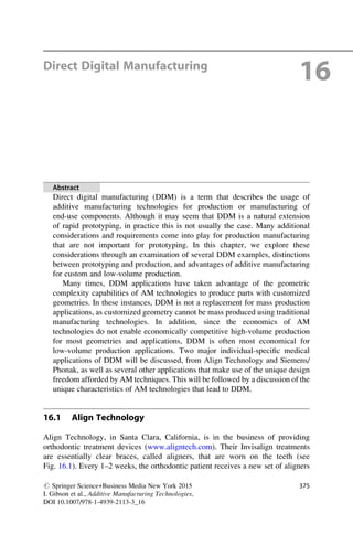
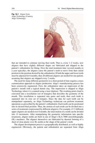
![Technology headquarters in California. Their data processing for the aligners is
performed in Costa Rica, translating customer-specific, doctor-prescribed tooth
movements into a set of aligner models. Each completed dataset is transferred
electronically to Align’s manufacturing facility in Juarez Mexico, where the dataset
is added into a build on one of their SL machines. After building the mold using VP
from the dataset, the molds are thermal formed. After thermal forming, they are
shipped back to Align and, from there, shipped to the orthodontist or the patient.
Between its founding in 1997 and March, 2009, over 44 million aligners have
been created (www.aligntech.com). At present, Align’s SL machines are able to
operate 24 h per day, producing approximately 100 aligner molds in one SLA-7000
build, with a total production capacity of 45,000–50,000 unique aligners per day
(~17 million per year) [1]. As each aligner is unique, they are truly “customized.”
And by any measure, 45,000 components per day is mass production and not
prototyping. Thus, Align Technology represents an excellent example of “mass
customization” using direct digital manufacturing (DDM), albeit in a tooling
application.
To achieve mass customization, Align needed to overcome the time-consuming
pre- and post-processing steps in SL usage. A customized version of 3D Systems
Lightyear control software was developed, called MakeTray; to automate most of
the build preparation. Aligner mold models are laid out, supports are generated,
process variables are set, and the models are sliced automatically. Typical post-
processing steps, including rinsing and post-curing can take hours. Instead, Align
developed several of its own post-processing technologies. They developed a
rinsing station that utilizes only warm water, instead of hazardous solvents. After
rinsing, conveyors transport the platforms to the special UV post-cure station that
Align developed. UV lamps provide intense energy that can post-cure an entire
platform in 2 min, instead of the 30–60 min that are typical in a Post-Cure
Apparatus unit. Platforms traverse the entire post-processing line in 20 min. Sup-
port structures are removed manually at present, although this step is targeted for
automation. The Align Technology example illustrates some of the growing pains
experienced when trying to apply technologies developed for prototyping to pro-
duction applications.
16.2 Siemens and Phonak
Siemens Hearing Instruments, Inc. (www.siemens-hearing.com) and Phonak
Hearing Systems are competitors in the hearing aid business. In the early 2000s,
they teamed up to investigate the feasibility of using polymer powder bed fusion
(PBF) technology in the production of shells for hearing aids [2]. A typical hearing
aid is shown in Fig. 16.2. The production of hearing aid shells (housings that fit into
the ear) required many manual steps. Each hearing aid must be shaped to fit into an
individual’s ear. Fitting problems cause up to 1 out of every 4 hearing aids to be
returned to the manufacturer, a rate that would be devastating in most other
industries.
16.2 Siemens and Phonak 377](https://image.slidesharecdn.com/1-230308091212-68402451/85/1-Additive-manufacturing-pdf-392-320.jpg)
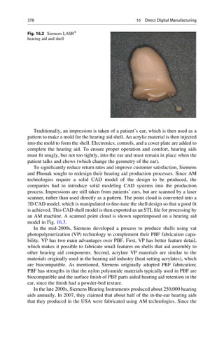
![introduction of AM-fabricated hearing aid shells, most hearing aid manufacturers in
the Western world have adopted AM in order to compete with Siemens and Phonak.
Recent surveys estimate that about 90 % of all custom in-the-ear hearing aid shells
are fabricated using AM, which totaled approximately two million AM fabricated
shells in 2012 [1]. Since the adoption of AM, hearing aid return rate has fallen
dramatically with improved design and manufacturing processes.
A number of technology advances have targeted this market. 3D Systems
developed a variant of its SLA Viper Si2 machine to manufacture shells, called
the SLA Viper HA. The machine contains two small vats, one with a red-tinted
resin and the other with a blue-tinted resin. The idea is to fabricate both the left and
right hearing aid shells for a patient in one build, where each shell is a different
color, enabling the patient to easily distinguish them. Of course, the resins can be
swapped with flesh-colored resin in both vats, if desired by a patient. EnvisionTEC
has also focused on this market, developing several VP machines that are designed
for hearing aid shells. Additionally, companies such as Rapid Shape, in Germany,
and Carima, in South Korea, have entered the market with mask projection VP
machines.
The hearing aid shell production is a great example of how companies can take
advantage of the shape complexity capability of RP technologies to economically
achieve mass customization. With improvements in scanning technology, it is
likely that patients’ ears can be scanned directly, eliminating the need for
impressions [3]. If desktop AM systems can be developed, it may even be possible
to fabricate custom hearing aids in the audiologist’s office, rather than having to
ship impressions or datasets to a central location!
Fig. 16.3 Hearing aid within
scanned point cloud
16.2 Siemens and Phonak 379](https://image.slidesharecdn.com/1-230308091212-68402451/85/1-Additive-manufacturing-pdf-394-320.jpg)
![16.3 Custom Footwear and Other DDM Examples
A British company called Prior 2 Lever (P2L) claims to be manufacturing the
world’s first custom soccer shoes for professional athletes. Polymer PBF is used to
fabricate the outsoles, including cleats, for individual customers [4]. The one-piece
leather uppers are also custom tailored. A model called the Assassin retailed in 2008
for £6,000 per pair; a photo is shown in Fig. 16.4. Research on PBF outsoles for
custom shoes started in the early 2000s at Loughborough University; Freedom of
Creation and others contributed to the development of this work. Early testing
demonstrated a significant reduction in peak pressures during walking and running
with personalized outsoles [5]. Custom sprinting shoes and triathlete shoes are also
being developed.
In 2013, Nike developed a line of football cleats called the Vapor Laser Talon.
The cleat plate was specially designed to improve player performance, particularly
for speed positions. It has an intricate, lattice design and was fabricating using PBF
in a proprietary polymer material.
The examples presented so far all relate to body-fitting, customized parts.
However, many other opportunities exist, even in the medical arena. Many
companies worldwide are investigating the use of PBF technologies for the creation
of orthopedic implants. For instance, Adler Ortho Group of Italy is using Arcam’s
EBM system to produce stock sizes of acetabular cups for hip implants made from
Ti–6Al–4V. The use of AM techniques enables a more compact design and a better
transition between the solid bearing surface and the porous bone-ingrowth portion
of the implant. Although a porous coating of titanium beads or hydroxyapatite on an
implant’s surface work well, they do not provide the optimum conditions for
osseointegration. The hierarchical structure capabilities of AM enable the creation
of a more optimal bone-ingrowth structure for osseointegration. As of early 2014,
more than 40,000 cups have been implanted and more than 90,000 implants have
been produced in series production by companies such as Adler Ortho and Lima
Corporate SpA. More generally, approximately 20 different AM medical implant
products have received FDA clearance for implantation in patients [1].
Fig. 16.4 Assassin model
soccer shoe. Courtesy prior
2 lever
380 16 Direct Digital Manufacturing](https://image.slidesharecdn.com/1-230308091212-68402451/85/1-Additive-manufacturing-pdf-395-320.jpg)
![Low-volume production is often economical via AM since hard tooling does not
need to be developed. This has led to the rapid adoption of DDM for low-volume
components across many industries. However, the most exciting aspects of DDM
are the opportunities to completely rethink how components can be shaped in order
to best fulfill their functions, as discussed in Chap. 13. Integrated designs can be
produced that combine several parts, eliminate assembly operations, improve
performance by designing parts to utilize material efficiently, eliminate shape
compromises driven by manufacturing limitations, and completely enable new
styles of products to be produced. This can be true for housewares, every-day
items, and even customized luxury items, as illustrated in Chap. 17 with respect
to houseware and fashion products. Each of these areas will be explored briefly in
this section. Many of the examples were taken, or cited, in recent Wohlers Reports
[1, 6].
Stratasys developed a new class of material extrusion (ME) machines in 2007,
the Fortus X00mc series. They introduced the Fortus 900mc in December and
reported that 32 parts on the machine were fabricated on their ME machines. This
is a novel example of how AM producers are using their own technologies in
low-volume production, and the savings that can be achieved by not having to
invest in tooling. Since introducing the 900mc, Stratasys has marketed several new
models, presumably using in-house fabricated parts on these models as well. This is
also true for other major AM manufacturers, including EOS and 3D Systems.
The aerospace industry has been the source of quite a few successful examples of
DDM. The F-18 fighter jet example from Chap. 17, where Boeing and Northrop
Grumman manufacture many nonstructural components using polymer PBF, is one
such case. In addition, SAAB Avitronics has used polymer PBF to manufacture
antenna RF boxes for an unmanned aircraft. Advantages of this approach over
conventional manufacturing processes include a more compact design, 45 % reduc-
tion in mass, and integral features. Paramount Industries, a division of 3D Systems,
produced PBF parts for a helicopter, including ventilation parts and electrical
enclosures, and structures for unmanned aerial vehicles. The parts were
manufactured on their EOSINT P 700 machine from EOS using the PA 2210 FR
material (flame retardant). Additionally, thousands of parts are flying on the space
shuttle, space station, and various military aircraft.
Many of the most promising commercial aircraft applications are delayed until
better flame retardant materials were certified for commercial use. Now, with flame
retardant PBF materials, Boeing has developed PBF components on commercial
737, 747 777, and 787 programs. In addition, large numbers of PBF components are
present on several military derivative aircrafts, such as the Airborne Early Warning
and Control (AEWC), C-40, AWACS, and P-8 aircraft. All told, tens of thousands
of parts are flying on at least eight different military and eight different civilian
models of Boeing aircraft. As another example, Northrop Grumman has identified
more than 1,400 parts on a single fighter aircraft platform that could be better made
using PBF than traditional methods if a suitable material with higher-temperature
properties were available.
16.3 Custom Footwear and Other DDM Examples 381](https://image.slidesharecdn.com/1-230308091212-68402451/85/1-Additive-manufacturing-pdf-396-320.jpg)
![Just as the development of computer graphics has often been driven by the gaming
industry, it is appearing equally likely that the further development of color DDM
technologies may also be driven by the market opportunities which are enabled by
the gaming industry. Quite a few online games allow players to create or customize
their own characters. Tools such as Maya are used to create/modify geometry,
colors, textures, etc. which are then uploaded to the game site (e.g., Dota 2 from
Valve). These same files can be packaged and sent to AM service providers, such as
Shapeways and Sculpteo, for printing color models of the custom characters. Make
Magazine ran a very informative article on this topic in 2013 [7].
In addition to the previous lines, many other DDM applications are emerging;
including in the medical and dental industries, which will be discussed further in
Chap. 15. Other examples are covered in Chaps. 2, 11 and 17.
16.4 DDM Drivers
It is useful to generalize from these examples and explore how the unique
capabilities of AM technologies may lead to new DDM applications. The factors
that enable DDM applications include:
• Unique Shapes: parts with customized shapes.
• Complex Shapes: improved performance.
• Lot Size of One: economical to fabricate customized parts.
• Fast Turnaround: save time and costs; increase customer satisfaction.
• Digital Manufacturing: precisely duplicate CAD model.
• Digital Record: have reusable dataset.
• Electronic “Spare Parts”: fabricate spare parts on demand, rather than holding
inventory.
• No Hard Tooling: no need to design, fabricate, and inventory tools; economical
low-volume production.
As indicated in the Align Technology and hearing aid examples, the capability to
create customized, unique geometries is an important factor for DDM. Many AM
processes are effective at fabricating platforms full of parts, essentially performing
mass customization of parts. For example, 100 aligner molds fit on one SLA-7000
platform. Each has a unique geometry. Approximately 25–30 hearing aid shells can
fit in the high-resolution region of an SLA Viper Si2 machine. Upwards of 4,000
hearing aid shells can be built in one PBF powder bed in one build. The medical
device industry is a leading—and growing—industry where DDM and rapid tooling
applications are needed due to the capability of fabricating patient-specific
geometries.
The capability of building parts with complex geometries is another benefit of
DDM. Features can be built into hearing aid shells that could not have been molded
in, due to constraints in removing the shells from their molds. In many cases, it is
possible to combine several parts into one DDM part due to AM’s complexity
16.4 DDM Drivers 383](https://image.slidesharecdn.com/1-230308091212-68402451/85/1-Additive-manufacturing-pdf-398-320.jpg)
![As mentioned several times, the advantages are numerous and significant to not
requiring tooling for part fabrication. Note that in cases such as Align Technology,
tooling is required, but the tooling itself is fabricated when and where needed, not
requiring tooling inventories. The elimination of tooling makes DDM economically
competitive across many applications for small lot size production.
16.5 Manufacturing Versus Prototyping
Production manufacturing environments and practices are much more rigorous than
prototyping environments and practices. Certification of equipment, materials, and
personnel, quality control, and logistics are all critical in a production environment.
Even small considerations like part packaging can be much different than in a
prototyping environment. Table 16.1 compares and contrasts prototyping and
production practices for several primary considerations [8].
Certification is critical in a production environment. Customers must have a
dependable source of manufactured parts with guaranteed properties. The DDM
company must carefully maintain their equipment, periodically calibrate the equip-
ment, and ensure it is always running within specifications. Processes must be
engineered and not left to the informal care of a small number of skilled technicians.
Experimentation on production parts is not acceptable. Meticulous records must be
kept for quality assurance and traceability concerns. Personnel must be fully
trained, cross-trained to ensure some redundancy, and certified to deliver quality
parts.
Most, if not all, DDM companies are ISO 9000 compliant or certified. ISO 9000
is an international standard for quality systems and practices. Most customers will
require such ISO 9000 practices so that they can depend on their suppliers. Many
books have been written on the ISO standards so, rather than go into extensive
detail here, readers should utilize these books to learn more about this topic [9].
As mentioned, personnel should be trained, certified, and periodically retrained
and/or recertified. Cross-training personnel on various processes and equipment
helps mitigate risks of personnel being unavailable at critical times. If multiple
shifts are run, these issues become more important, since the quality must be
consistent across all shifts.
Vertical integration is important, since many customers will want their suppliers
to be “one stop shops” for their needs. DDM companies may rely on their own
suppliers, so the supplier network may be tiered. It is up to the DDM company,
however, to identify their suppliers for specialty operations, such as bonding,
coating, and assembly, and ensure that their suppliers are certified.
The bottom line for a company wanting to break into the DDM industry is that
they must become a production manufacturing organization, with rigorous
practices. Having an informal, prototyping environment, even if they can produce
high-quality prototypes, is not sufficient for success in the current DDM industry.
Standard production business practices must be adopted.
16.5 Manufacturing Versus Prototyping 385](https://image.slidesharecdn.com/1-230308091212-68402451/85/1-Additive-manufacturing-pdf-400-320.jpg)
![Several industry standards, e.g., ISO 9000, have been available to assist
companies in adopting quality and certification best practices. Until recently, few
AM-specific standards were available, which meant that:
• Material data reported by various companies are not comparable.
• Technology users employ different process parameters to operate their equip-
ment according to their own preferences.
• There is little repeatability of results between suppliers or service bureaus.
• There are few specifications which can be referenced by end users to help them
ensure that a product is built as-desired.
In 2008, an international standards-development initiative was organized by the
Society of Manufacturing Engineering; ASTM International was selected to be the
organization that the AM community would work with to develop standards. The
first meeting of the ASTM F42 committee on standards for Additive Manufacturing
Technologies was held in May, 2009. At present, several standards have been
Table 16.1 Contrast between rapid prototyping and direct digital manufacturinga
Key
characteristic RP company DDM company
Certification
Equipment From equipment manufacturer Production machines and calibration
equipment
Personnel No formal testing, certification, or
training typical
On-going need for certification
Practices Trial-and-error, no formal
documentation of practices
Formal testing for each critical step,
periodic recertification
Quality Basic procedures; some inspection ISO 9000 compliance. Extensive,
thorough quality system needed
Manufacturing
System Basic system; controls and
documentation not essential
Developed system; controls and
documentation required
Planning Basic. Requires only modest part
assessment
Formal planning to ensure customer
requirements are met. Developed
process chains, no experimentation
Scheduling
and
delivery
Informally managed; critical jobs
can be expedited; usually only one
delivery date
Sophisticated scheduling, just-in-time
delivery
Personnel Informal training, on-the-job
training; certification not necessary;
redundancy not essential
Formal training for certification and
periodic recertification. Redundant
personnel needed for risk mitigation
Vertical
integration
Helpful From customer’s perspective, should
be a one-stop-shop. Qualified
suppliers must be lined up ahead of
time to enable integration
a
Much of this section was adapted from Brian Hasting’s presentation at the 2007 SME RAPID
Conference [8]
386 16 Direct Digital Manufacturing](https://image.slidesharecdn.com/1-230308091212-68402451/85/1-Additive-manufacturing-pdf-401-320.jpg)
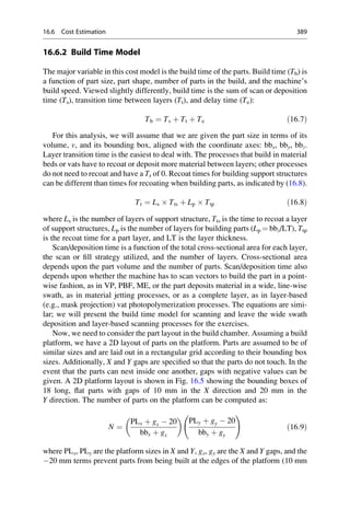
![buffer area along each platform edge). This analysis can be extended to 3D build
chambers for processes which enable stacking in the z direction.
The time to scan one part depends on the part cross-sectional area, the laser or
deposition head diameter d, the distance between scans h, and the average scan
speed ssavg. Cross-sectional area, Aavg, is approximated by using an area correction
factor γ [10], which corrects the area based on the ratio of the actual part volume to
the bounding box volume, vbb, γ ¼ v/vbb. The following correction has been shown
to give reasonable results in many cases.
Afn ¼ γ eα 1γ
ð Þ
ð16:10Þ
Aavg ¼ bbx bby Afn ð16:11Þ
where α is typically taken as 1.5.
For scanning processes, it is necessary to determine the total scan length per
layer. This can be accomplished by simply dividing the cross-sectional area by the
diameter of the laser beam or deposited filament. Alternatively, the scan length can
be determined by dividing the cross-sectional area by the hatch spacing (distance
between scans). We will use the latter approach, where the hatch spacing, hr, is
given as a percentage of the laser beam diameter. For support structures, we will
assume that the amount of support is a constant percentage, supfac, of the cross-
sectional area (assumed as about 30 %). If a process does not require supports, then
the constant percentage can be taken as 0. The final consideration is the number of
times a layer is scanned to fabricate a layer, denoted nst. For example, in
stereolithography, both X and Y scans are performed for each layer, while in
Fig. 16.5 SLA-7000 vat with 18 parts laid out on the platform
390 16 Direct Digital Manufacturing](https://image.slidesharecdn.com/1-230308091212-68402451/85/1-Additive-manufacturing-pdf-405-320.jpg)
![material extrusion, only one scan is performed to deposit material. Scan length for
one part and its support structure is determined using (16.12):
sl ¼ Aavg
nstLp
hr d
þ supfac
Ls
d
ð16:12Þ
The final step in determining scan/deposition time is to determine scan speed. This
is a function of how fast the laser or deposition head moves when depositing
material, sss, as well as when moving (jumping) between scans, ssj. In some
cases, jump speed is much higher than typical scan speeds. To complicate this
matter, many machines have a wide range of scan speeds that depend on several
part building details. For example, new VP machines have scan speeds that range
from 100 to 25,000 mm/s. For our purposes, we will assume a typical scan speed
that is half of the maximum speed. The average scan/deposition speed will be
corrected using the area correction factor determined earlier [10] as
ssavg ¼ sss γ þ ssj 1 γ
ð Þ ð16:13Þ
With the intermediate terms determined, we can compute the scan/deposition time
for all parts in the build as:
Ts ¼
N sl
3, 600 ssavg
ð16:14Þ
where the 3,600 in the denominator converts from seconds to hours.
The final term in the build time expression (16.7) is the delay time, Te. Many
processes have delays built into their operations, such as platform move time,
pre-recoat delay (Tpredelay), post-recoat delay (Tpostdelay), nozzle cleaning, sensor
recalibration, temperature set point delays (waiting for the layer to heat or cool to
within a specified range), and more. These delays are often user specified and
depend upon build details for a particular process. For example, in VP, if parts
have many fine features, longer pre-recoat delays may be used to allow the resin to
cure further, to strengthen the part, before subjecting fragile features to recoating
stresses. Additionally, some processes require a start-up time, for example, to heat
the build chamber or warm up a laser. This start-up time will be denoted Tstart. For
our purposes, delays will be given by (16.15), but it is important to realize that each
process and machine may have additional or different delay terms.
Te ¼ Lp Tpredelay þ Tpredelay
þ Tstart ð16:15Þ
With the cost and build time models presented, we now turn to the application of
these models to VP.
16.6 Cost Estimation 391](https://image.slidesharecdn.com/1-230308091212-68402451/85/1-Additive-manufacturing-pdf-406-320.jpg)

![presented. The chapter concludes with a discussion of design synthesis approaches
to optimize designs.
17.2 Design for Manufacturing and Assembly
Design for manufacturing and assembly can be defined as the practice of designing
products to reduce, and hopefully minimize, manufacturing and assembly
difficulties and costs. This makes perfectly good sense, as why would one want to
increase costs? However, DFM requires extensive knowledge of manufacturing and
assembly processes, supplier capabilities, material behavior, etc. DFM, although
simple conceptually, can be difficult and time consuming to apply. To achieve the
objectives of DFM, researchers and companies have developed a large number of
methods, tools, and practices. Our purpose in this chapter is not to cover the wide
spectrum of DFM advances; rather, it is to convey a sense of the variety of DFM
approaches so that we can compare and contrast DFAM with DFM.
Broadly speaking, DFM efforts can be classified into three categories:
• Industry practices, including reorganization of product development using
integrated product teams, concurrent engineering, and the like
• Collections of DFM rules and practices
• University research in DFM methods, tools, and environments
During the 1980s and 1990s, much of the product development industry
underwent significant changes in structuring product development organizations
[1]. Companies such as Boeing, Pratt Whitney, and Ford reorganized product
development into teams of designers, engineers, manufacturing personnel, and
possibly other groups; these teams could have hundreds or even thousands of
people. The idea was to ensure good communication among the team so that design
decisions could be made with adequate information about manufacturing processes,
factory floor capabilities, and customer requirements. Concurrently, manufacturing
engineers could understand decision rationale and start process planning and
tooling development to prepare for the in-progress designs. A significant driver of
this restructuring was to identify conflicts early in the product development process
and reduce the need for redesign or, even worse, retooling of manufacturing
processes after production starts.
The second category of DFM work, that of DFM rules and practices, is best
exemplified by the Handbook for Product Design for Manufacture [2]. The 1986
edition of this handbook was over 950 pages long, with detailed descriptions of
engineering materials, manufacturing processes, and rules-of-thumb. Extensive
examples of good and bad practices are offered for product design for many of
these manufacturing processes, such as molding, stamping, casting, forging,
machining, and assembly.
University research during the 1980s and 1990s started with the development of
tools and metrics for part manufacture and assembly. The Boothroyd and Dewhurst
17.2 Design for Manufacturing and Assembly 401](https://image.slidesharecdn.com/1-230308091212-68402451/85/1-Additive-manufacturing-pdf-415-320.jpg)
![toolkit is probably the most well-known example [3]. The main concept was to
develop simple tools for designers to evaluate the manufacturability of their
designs. For example, injection molding DFM tools were developed that asked
designers to identify how many undercuts were in a part, how much geometric
detail is in a part, how many tight tolerances were needed, and similar information.
From this information, the tool provided assessments of manufacturability
difficulties, costs estimates, and provided some suggestions about part redesign.
Similar tools and metrics were developed for many manufacturing and assembly
processes, based in part on the Handbook mentioned above, and similar collections
of information. Some of these tools and methods were manual, while others were
automated; some were integrated into CAD systems and performed automated
recognition of difficulties. For instance, Boothroy Dewhurst, Inc. markets a set of
software tools that help designers conceive and modify their design to achieve
lower-cost parts, taking into account the specific manufacturing process being
utilized. In addition, they sell software tools which help designers improve the
design of assembled components through identification of the key functional
requirements of an assembled component; leading the designer through a process
of design modifications with the aim of minimizing the number of parts and
assembly operations used to create that assembled component. The work in this
area is extensive; see for example, the ASME Journal of Mechanical Design and the
ASME International Design Engineering Technical Conferences proceedings since
the mid-1980s (see e.g., [4]).
The extensive efforts on DFM over many years are an indication of the difficulty
and pervasiveness of the issues surrounding DFM. In effect, DFM is about the
designer understanding the constraints imposed by manufacturing processes, then
designing products to minimize constraint violation. Some of these difficulties are
lessened when parts are manufactured by AM technologies, but some are not.
Integrated product development teams that practice concurrent engineering make
sense, regardless of intended manufacturing processes. Rules, methods, and tools
that assist designers in making good decisions about product manufacturability
have a significant role to play. However, the nature of the rules, methods, and tools
should change to assist designers in understanding the design freedom allowed by
AM and, potentially, aiding the designer in exploring the resulting open design
spaces, while ensuring that manufacturing constraints (yes, AM technologies do
have constraints) are not violated.
To illustrate the differences between DFM and DFAM, this section will con-
clude with two examples. The first involves typical injection molding
considerations, that of undercuts and feature detail. Consider the camera spool
part shown in Fig. 17.1 [5]. The various ribs and pockets are features that contribute
to the time and cost of machining the mold in which the spools will be molded. Such
feature detail is not relevant to AM processes since ribs can be added easily during
processing in an AM machine. A similar result relates to undercuts. This spool
design has at least one undercut, since it cannot be oriented in a mold consisting of
only two mold pieces (core and cavity), while enabling the mold halves to be
separated and the part removed. Most probably, the spool will be oriented so that
402 17 Design for Additive Manufacturing](https://image.slidesharecdn.com/1-230308091212-68402451/85/1-Additive-manufacturing-pdf-416-320.jpg)
![the mold closure direction is parallel to the walls of the ribs. In this manner, the core
and cavity mold halves form most of the spool features, including the ribs
(or pockets), the flanges near the ends, and the groove seen at the right end. In
this orientation, the hole in the right end cannot be formed using the core and/or
cavity. A third moving mold section, called a side action, is needed to form the hole.
In AM processes, it is not necessary to be so concerned about the relative position
and orientation of features, since, again, AM machines can fabricate features
regardless of their position in the part.
In design for assembly, two main considerations are often offered to reduce
assembly time, cost, and difficulties: minimize the number of parts and eliminate
fasteners. Both considerations translate directly to fewer assembly operations, the
primary driver for assembly costs [3]. To minimize parts and fasteners, integrated
part designs typically become much more complex and costly to manufacture.
Design for manufacture and design for assembly will often be repeated, iteratively,
until an optimal solution is found; one where the increasing manufacturing costs for
more complex components are no longer compensated by the assembly cost
savings.
The designs in Fig. 17.2 show two very different approaches to designing ducts
for aircraft [6, 7]. This example represents a design concept for conveying cooling
air to electronic units in military aircraft, but could apply to many different
applications. The first design is a typical approach using parts fabricated by
conventional manufacturing processes (stamping, sheet metal forming, assembly
using screws, etc.). In contrast, the approach on the right illustrates the benefits of
taking design for assembly guidelines to their extreme: the best way to reduce
assembly difficulties and costs is to eliminate assembly operations altogether! The
resulting design replaces 16 parts and fasteners with 1 part that exhibits integrated
flow vanes and other performance enhancing features. However, this integrated
design cannot be fabricated using conventional manufacturing techniques and is
only manufacturable using AM.
Fig. 17.1 Camera spool
example
17.2 Design for Manufacturing and Assembly 403](https://image.slidesharecdn.com/1-230308091212-68402451/85/1-Additive-manufacturing-pdf-417-320.jpg)
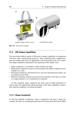
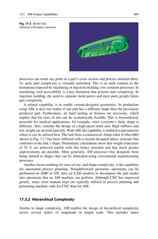
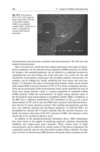
![achievable. Similarly, by varying either the materials present (when using a
multimaterial AM system) or the processing of the materials, this type of nano/
microstructure control is also possible in ME, material jetting, VP, and sheet
lamination AM technologies as well. These related possibilities are further explored
below with respect to material complexity.
The ability to change the mesostructure of a part is typically associated with the
application of cellular structures, such as honeycombs, foams, or lattices, to fill
certain regions of a geometry. This is often done to increase a part’s strength to
weight or stiffness to weight ratio. These structures are discussed in more detail in
Sect. 17.5.2.
When considered together, the ability to simultaneously control a part’s nano/
microstructure, mesostructure, and macrostructure simply by changing process
parameters and CAD data is a capability of AM which is unparalleled using
conventional manufacturing.
17.3.3 Functional Complexity
When building parts in an additive manner, one always has access to the inside of
the part. Two capabilities are enabled by this. First, by carefully controlling the
fabrication of each layer, it is possible to fabricate operational mechanisms in some
AM processes. By ensuring that clearances between links are adequate, revolute or
translational joints can be created. Second, components have been inserted into
parts being built in VP, ME, PBF, sheet lamination, and other AM machines,
enabling in situ assembly.
A wide variety of kinematic joints has been fabricated directly in VP, ME, and
PBF technologies, including vertical and horizontal prismatic, revolute, cylindrical,
spherical, and Hooke joints. Figure 17.5 shows one example of a pulley-driven,
snake-like robot with many revolute joints that was built as assembled in the
SLA-3500 machine at Georgia Tech.
Similar studies have been performed using material extrusion (ME) and PBF
processes. The research group at Rutgers University led by Dr. Mavroidis [8]
demonstrated that the same joint geometries could be fabricated by both ME and
PBF machines and similar clearances were needed in both machine types. In PBF,
Fig. 17.5 Pulley-driven
snake-like robot
17.3 AM Unique Capabilities 407](https://image.slidesharecdn.com/1-230308091212-68402451/85/1-Additive-manufacturing-pdf-421-320.jpg)
![loose powder must be removed from the joint locations to enable relative joint
motion. In ME, the usage of soluble support material ensures that joints can be
movable after post-processing in a suitable solvent.
In the construction of functional prototypes, it is often advantageous to embed
components into parts while building them in AM machines. This avoids post-
fabrication assembly and can greatly reduce the number of separate parts that have
to be fabricated and assembled.
For example, it is possible to fabricate VP devices with a wide range of
embedded components, including small metal parts (bolts, nuts, bushing), electric
motors, gears, silicon wafers, printed circuit boards, and strip sensors. Furthermore,
VP resins tend to adhere well to embedded components, reducing the need for
fasteners. Shown in Fig. 17.6 is a model of an SLA-250 machine that was built in
the SLA-250 at Georgia Tech [9]. This 150 150 260 mm model was built at 1:¼
scale, with seven inserted components, four sliding contact joints, and one rotating
contact joint. The recoating blade slides back-and-forth across the vat region,
driven by an electric motor and gear train. Similarly, the elevator and platform
translate vertically, driven by a second electric motor and leadscrew. The laser
pointer and galvanometers worked to draw patterns on the platform, but these three
components were assembled after the build, rather than subjecting them to being
dipped into the resin vat. Build time was approximately 75 h, including time to
pause the build and insert components.
Other researchers have also demonstrated the capability of building functional
devices, including the Mavroidis group and Dr. Cutkosky’s group at Stanford
University [10]. Device complexity is greatly facilitated when the capability to
Motor
Leadscrew part 2 Bushing 2
Bushing 1
Galvanometers
Laser
Nut
Leadscrew part 1
Motor for
recoating
mechanism
Left right sliding contact joints
of recoater assembly
Left right sliding contact
joints of elevator assembly
Rotating
contact joints
Rack for
recoating
mechanism
David Rosen Brent Stucker
Fig. 17.6 SLA-250 model built in an SLA-250 machine with 11 embedded components
408 17 Design for Additive Manufacturing](https://image.slidesharecdn.com/1-230308091212-68402451/85/1-Additive-manufacturing-pdf-422-320.jpg)
![fabricate kinematic joints is coupled with embedded inserts since functional
mechanisms can be fabricated entirely within the VP vat, greatly simplifying the
prototyping process.
Functional complexity can also be achieved by unique combination of AM
technologies to produce, for instance, 3D integrated electronics. Researchers in
the W.M. Keck Center for 3D Innovation at the University of Texas at El Paso have
demonstrated the ability to produce a number of working devices by novel
combinations of VP or ME and DW. Figure 17.7 illustrates the process plan for
fabrication of a magnetic flux sensor using VP and a nozzle-based DW process.
Researchers have demonstrated similar capabilities with ME, sheet lamination,
PBF, and other technologies as well.
17.3.4 Material Complexity
Since material is processed point to point in many of the AM technologies, the
opportunity is available to process the material differently at different points, as
illustrated above, causing different material properties in different regions of the
part. In addition, many AM technologies enable changing material composition
gradually or abruptly during the build process. New applications will emerge to
take advantage of these characteristics.
The concept of functionally graded materials, or heterogeneous materials, has
received considerable attention [11], but manufacturing useful parts from these
materials often has been problematic. Consider a turbine blade for a jet engine. The
Fig. 17.7 Fabrication of a magnetic flux sensor using VP and DW (courtesy of W.M. Keck Center
for 3D Innovation at The University of Texas at El Paso)
17.3 AM Unique Capabilities 409](https://image.slidesharecdn.com/1-230308091212-68402451/85/1-Additive-manufacturing-pdf-423-320.jpg)
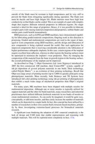
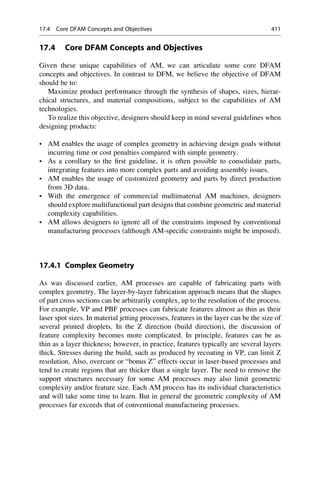
![17.4.2 Integrated Assemblies
The capability for complex geometry enables other practices. As was demonstrated
at the end of Sect. 17.2, several parts can be replaced with a single, more complex
part in many cases. Even when two or more components must be able to move with
respect to one another, such as in a ball-and-socket joint, AM can build these
components fully assembled. These capabilities enable the integration of features
from multiple parts, possibly yielding better performance. Additionally, a reduction
in the number of assembly operations can have a tremendous impact on production
costs and difficulties for products.
As is evident from conventional DFM practices, design changes to facilitate or
eliminate assembly operations can lead to much larger reductions in production
costs than changes to facilitate part manufacture [3]. This is true, at least in part, due
to the elimination of any assembly tooling that may have been required. Although
conventional DFM guidelines for part manufacturing are not relevant to AM, the
design-for-assembly guidelines remain relevant and perhaps even more important.
Other advantages exist for the consolidation of parts. For example, a reduction in
part count reduces product complexity from management and production
perspectives. Fewer parts need to be tracked, sourced, inspected, etc. The need
for spare or replacement parts decreases. Furthermore, the need to warehouse
tooling to fabricate the parts can be eliminated. In summary, part consolidation
can lead to significant savings across the entire enterprise.
17.4.3 Customized Geometry
Consistent with the capability of complex geometry, AM processes can fabricate
custom geometries. This has been demonstrated by a series of examples throughout
this book related to direct digital manufacturing and biomedical applications. A
good example is that of hearing aid shells (Sect. 16.2). Each shell must be
customized for an individual’s particular ear canal geometry. In VP or PBF
machines, hundreds or thousands of shells, each of a different geometry, can be
built at the same time in a single machine. Mass customization, instead of mass
production, can be realized quite readily. The lack of generic software tools for
mass customization, rather than limitations of the hardware, is the key limitation
when considering AM for mass customization.
17.4.4 Multifunctional Designs
Multifunctionality is simply the achievement of multiple functions, or purposes,
with a single part. This is commonly achieved when performing part consolidation,
but the capability of material complexity enables much more ambitious
explorations of design possibilities. For example, if a part needs to be stiff in one
location, but flexible in another, several AM processes could be used to fabricate
412 17 Design for Additive Manufacturing](https://image.slidesharecdn.com/1-230308091212-68402451/85/1-Additive-manufacturing-pdf-426-320.jpg)
![17.5.1 Part Consolidation and Redesign
The characteristics of geometric complexity and suitability for low-volume produc-
tion combine to yield substantial benefits in many cases for consolidating parts into
a smaller number of more complex parts that are then fabricated using an AM
process. This has several significant advantages over designs with multiple parts.
First, dedicated tooling for multiple parts is not required. Potential assembly
difficulties are avoided. Assembly tooling, such as fixtures, is not needed. Fasteners
can often be eliminated. Finally, it is often possible to design the consolidated parts
to perform better than the assemblies.
A well-known example that illustrates these advantages was shown in Fig. 17.2,
that of a prototypical duct for military aircraft [6, 7]. The design shows a typical
traditional design with many formed and rotomolded plastic parts, some formed
sheet-metal parts, and fasteners [12]. The example was from the pioneering work of
the Boeing Phantom Works Advanced Direct Digital Manufacturing group in
retrofitting F-18 fighter jets with dozens of parts produced using PBF. Many of
these parts replaced standard ducting components to deliver cooling air to electron-
ics modules. Significant part reductions, elimination of fasteners, and optimization
of shapes are illustrative of the advances made by Boeing. Through these methods,
many part manufacturing tools and assembly operations were eliminated.
A second example, from Loughborough University, illustrates the advantages of
reconceptualizing the design of a component based on the ability to avoid
limitations of conventional manufacturing processes. Figure 17.8 shows a front
plate design for a diesel engine [7]. The channels through which fuel or oil flow are
gun drilled. As a result, they are straight; furthermore, plugs need to be added to
plug up the holes through the housing that enabled the channels to be drilled. The
redesign shown in Fig. 17.8b was developed by designing the flow channels to
ensure efficient flows, then adding a minimal amount of additional material to
provide structural integrity. As a result, the part is smaller, lighter, and has better
performance than the original design.
Fig. 17.8 Diesel front plate example. (a) Original design. (b) Redesigned for additive
manufacturing
414 17 Design for Additive Manufacturing](https://image.slidesharecdn.com/1-230308091212-68402451/85/1-Additive-manufacturing-pdf-428-320.jpg)
![17.5.2 Hierarchical Structures
The basic idea of hierarchical structures is that features at one size scale can have
smaller features added to them, and each of those smaller features can have smaller
features added, etc. Tailored nano/microstructures are one example. Textures added
to surfaces of parts are another example. In addition, cellular materials (materials
with voids), including foams, honeycombs, and lattice structures, are a third
example of hierarchical feature. To illustrate the benefits of designing with hierar-
chical flexibility, we will focus on cellular materials in this section.
The concept of designed cellular materials is motivated by the desire to put
material only where it is needed for a specific application. From a mechanical
engineering viewpoint, a key advantage offered by cellular materials is high
strength accompanied by a relatively low mass. These materials can provide good
energy absorption characteristics and good thermal and acoustic insulation
properties as well [13]. When the characteristic lengths of the cells are in the
range of 0.1–10 mm, we refer to these materials as mesostructured materials.
Mesostructured materials that are not produced using stochastic processes (e.g.,
foaming) are called designed cellular materials.
In the past 15 years, the area of lattice materials has received considerable
attention due to their inherent advantages over foams in providing light, stiff, and
strong materials [14]. Lattice structures tend to have geometry variations in three
dimensions; as is illustrated in Fig. 17.9. As pointed out in [15], the strength of
foams scales as ρ1.5
, whereas lattice structure strength scales as ρ, where ρ is the
volumetric density of the material. As a result, lattices with a ρ ¼ 0.1 are about three
times stronger per unit weight than a typical foam. The strength differences lie in
the nature of material deformation: the foam is governed by cell wall bending,
while lattice elements stretch and compress. The examples shown in Fig. 17.9
utilize the octet-truss (shown on the left), but many other lattice structures have
been developed and studied (e.g., kagome, Kelvin foam) [16, 17].
cylinder with 2 layers of truss
structure made in SL
1
1
1
0.5
0.5
0.5
octet-truss
u
v
d
a
b c
w
0
0
0
skin with single layer of lattice structure
Fig. 17.9 Octet-truss unit cell and example parts with octet-truss mesostructures
17.5 Exploring Design Freedoms 415](https://image.slidesharecdn.com/1-230308091212-68402451/85/1-Additive-manufacturing-pdf-429-320.jpg)
![The parts shown in Fig. 17.9b, c illustrate one method of developing stiff,
lightweight structures, that of using a thin part wall, or skin, and stiffening it with
cellular structure. Another method could involve filling a volume with the cellular
structures. Using either approach often results in part designs with thousands of
shape elements (beams, struts, walls, etc.). Most commercial CAD systems cannot
perform geometric modeling operations on designs with more than 1,000–2,000
elements. As a result, the design in Fig. 17.9c, which has almost 18,000 shape
elements, cannot be modeled using conventional CAD software. Instead, new CAD
technologies must be developed that are capable of modeling such complex
geometries [18]; this is the subject of Sect. 17.6.
Several groups designed unmanned aerial vehicles (UAV) components by
applying various cellular structure design approaches. Figure 17.10 shows a hand-
held UAV, the Streetflyer from AVID LLC, that was redesigned to utilize lattice
structure reinforcement. The original design of the UAV utilized carbon fiber skins
Fig. 17.10 Lattice structure-based UAV design. (a) lattice structure designs for fuselage and
wings. (b) assembled UAV ready for test flight
416 17 Design for Additive Manufacturing](https://image.slidesharecdn.com/1-230308091212-68402451/85/1-Additive-manufacturing-pdf-430-320.jpg)
![for the fuselage and wings, but required many assembly operations to add stiffeners,
fastening features, and mounting features to the components. In contrast, by
designing for AM, the lattice structure-based design had such features and stiffeners
designed in. Experts at Paramount Industries, a 3D Systems company, fabricated
the fuselage and wings in Duraform using PBF. Test flights demonstrated that the
PBF-fabricated UAV performed well and, even though the UAV was not
optimized, its performance approached that of the carbon fiber production version.
17.5.3 Industrial Design Applications
Some very intriguing approaches to product design have been demonstrated that
take advantage of the shape complexity capabilities of AM, as well as some
material characteristics. A leader in this field was a small company in The
Netherlands called Freedom of Creation (FOC), founded by Janne Kytannen,
which was purchased by 3D Systems in the early 2010s. See: http://www.
freedomofcreation.com.
FOC began operations in the late 1990s. Their first commercial products were
lamp shades fabricated in VP and PBF [20], an example of which is shown in
Fig. 17.11a. They have since developed many families of lampshade designs. In
2003, they partnered with Materialise to market lampshades, which retail for 300 to
6,000 euros (as of 2009).
Many other classes of products have been developed, including chairs and
stools, handbags, bowls, trays, and other specialty items. See Fig. 17.11b, c for
examples of other products. Also, they have partnered with large and small
organizations to develop special “give-aways” for major occasions, many of
which were designed to be manufactured via AM.
In the early 2000s, they developed the concept of manufacturing textiles. Their
early designs were of chain-mail construction, manufactured in PBF. Since then,
they have developed several lines of products using similar concepts, including
handbags, other types of bags, and even shower scrubs.
More recently, quite a few other companies have demonstrated very innovative
designs of housewares, clothing, fashion accessories, and even shoes. Fashion
shows have focused on AM-fabricated clothes, parts of clothing, and accessories.
Some examples from 2014 include Anouk Wipprecht’s electrified 3D printed
dresses, hats/headpieces by Gabriela Ligenza, Ray Civello, and Stephen Ma, and
dresses and accessories from Iris Van Herpen.
Another source of inspiration comes from browsing the virtual storefronts on
shapeways.com and ponoko.com, where individual entrepreneurs and small
companies can offer custom designs. Everything from jewelry to candle holders
to bird houses can be found on these sites. Methods of manufacturing the designs
offered on each storefront need to be provided and many times the only methods are
through AM. Some sites provide design guidelines, suggestions, or even specially
developed CAD tools.
17.5 Exploring Design Freedoms 417](https://image.slidesharecdn.com/1-230308091212-68402451/85/1-Additive-manufacturing-pdf-431-320.jpg)
![planning and other analysis activities. Potentially, this issue will slow the adoption
of AM technologies for use in production manufacture. More specifically, the
challenges for CAD can be stated as:
• Geometric complexity—need to support models with tens and hundreds of
thousands of features.
• Physically based material representations—material compositions and
distributions must be represented and must be physically meaningful.
• Physically based property representations—desired distributions of physical and
mechanical properties must be represented and tested for their physical basis.
One example of the geometric complexity issue is illustrated by the prototype
textile application, from Loughborough University and Freedom of Creation,
shown in Fig. 17.12 [21]. On the left is a “chain mail”-like configuration of many
small rings. On the right is an example garment fabricated on a PBF machine in a
Duraform material. The researchers desired to fold up the CAD model of the
garment so that it occupied a very small region in the machine’s build platform,
which would maximize the throughput of the PBF machine for production
purposes. The Loughborough researchers had great difficulty modeling the collec-
tion of thousands of rings that comprise the garment in a commercial solid-
modeling CAD system. Instead they developed their own CAD system for textile
and similar structured surface applications over several years. However, having to
develop custom CAD systems for specific applications will be a significant barrier
to widespread adoption of AM.
Two CAD challenges can be illustrated by some simple examples. The Stratasys
Connex 500 material jetting machine can deposit several different materials while
building one part. To drive the machine, Stratasys needed to develop a new
Fig. 17.12 Example of textiles produced using PBF
17.6 CAD Tools for AM 419](https://image.slidesharecdn.com/1-230308091212-68402451/85/1-Additive-manufacturing-pdf-433-320.jpg)
![software tool that allows users to specify materials in different regions of STL files.
It would be far better to be able to specify material composition in the original CAD
system, so that vendor or machine-specific tools are not needed. The second
example was a research project from the Fraunhofer Institute for Manufacturing
and Advanced Materials (IFAM) in Bremen, Germany [22]. They developed a
two-binder system for 3D Printing technology, where one binder is traditional and
one is carbon laden. Their goal was to produce gradient strength steel parts by
depositing the carbon according to a desired distribution of hardness. The model of
hardness will be converted into a representation of carbon distribution, which will
be converted into carbon-laden binder deposition commands for the 3DP system.
After building, the part will be heat treated to diffuse the carbon into the steel. As a
result, this application illustrates the need to represent distributions of mechanical
properties (hardness) and material composition (carbon, steel), and relate these to
processing conditions. The IFAM researchers developed a software system for this
application.
17.6.2 Solid-Modeling CAD Systems
Parametric, solid-modeling CAD systems are used throughout much of the world
for mechanical product development and are used in university education and
research. Such systems, such as ProEngineer, Unigraphics, SolidEdge, CATIA,
and SolidWorks, are very good for representing shapes of most engineered parts.
Their feature-based modeling approaches enable fast design of parts with many
types of typical shape elements. Assembly modeling capabilities provide means for
automatically positioning parts within assemblies and for enforcing assembly
relationships when part sizes are changed.
Commercial CAD systems typically have a hybrid CSG-BRep (constructive
solid geometry—boundary representation) internal representation of part geometry
and topology. With the CSG part of the representation, part construction history is
maintained as a sequence of feature creation, operation, and modification processes.
With the BRep part of the representation, part surfaces are represented directly and
exactly. Adjacencies among all points, curves, surfaces, and solids are maintained.
A tremendous amount of information is represented, all of which has its purposes
for providing design interactions, fast graphics, mass properties, and interfaces to
other CAD/CAM/CAE tools.
For parts with dozens or hundreds of surfaces, commercial CAD systems run
with interactive speeds, for most types of design operations, on typical personal
computers. When more than 1,000 surfaces or parts are modeled, the CAD systems
tend to run very slowly and use hundreds of MB or several GB of memory. For the
textile part, Fig. 17.12, thousands of rings comprise the garment. However, they
have the same simple shape, that of a torus. A different type of application is that of
hierarchical structures, where feature sizes span several orders of magnitude. An
example is that of a multimaterial mold with conformal cooling channels, where the
cooling channels have small fins or other protrusions to enhance heat transfer. The
420 17 Design for Additive Manufacturing](https://image.slidesharecdn.com/1-230308091212-68402451/85/1-Additive-manufacturing-pdf-434-320.jpg)
![fins or protrusions may have sizes of 0.01 mm, while the channels may be 10 mm in
diameter, and the mold may be 400 mm long. The central region of the mold may
use a high conductivity, high toughness material composition, whereas the surface
of the mold may have a high hardness material composition, where a conformal,
gradient transition occurs within a region near the surface of the mold. As a result,
the mold model may have many thousands of small features and must also represent
a gradient material composition that is derived from knowledge of the geometric
features. In addition, the range of size scales may cause problems in managing
internal tolerances in the CAD system. Current CAD systems are incapable of
representing the thousands of features or the graded material composition o f this
mold example.
In summary, two main geometry-related capabilities are needed to support many
emerging design applications, particularly when AM manufacturing processes will
be utilized:
• Representation of tens or hundreds of thousands of features, surfaces, and parts.
• Managing features, materials, surfaces, and parts across size ranges of 4–6
orders of magnitude.
The ISO STEP standard provides a data exchange representation for solid
geometry, material composition, and some other properties. However, it is intended
for exchanging product information among CAD, CAM, and CAE systems, not for
product development and manufacturing purposes. That is, the STEP representation
was not developed for use within modeling and processing applications. A good
assessment of its usefulness in representing parts with heterogeneous materials for
AM manufacturing is given in reference [11], although at present the standards
community is revisiting the potential usage of STEP for AM.
As mentioned above, the first challenge for CAD systems is geometric complex-
ity. The second challenge for CAD systems is to directly represent materials, to
specify a part’s material composition. As a result, CAD models cannot be used to
represent parts with multiple materials or composite materials. Material composi-
tion representations are needed for parts with graded interfaces, functionally graded
materials, and even simpler cases of particle or fiber filler materials. Furthermore,
CAD models can only provide geometric information for other applications, such as
manufacturing or analysis, not complex multiple material information, which limits
their usefulness. This type of limitation is clear when one considers the ink-jet
printing examples mentioned so far (e.g., Stratasys multimaterial printer, IFAM
carbon-laden inks). In the IFAM case, the addition of carbon to steel deals with the
relatively well understood area of carbon steels. In other applications, novel
material combinations that are less understood may be of interest. Two main issues
arise, including the need to:
• Represent desired material compositions at appropriate size scales.
• Determine the extent to which desired material compositions are achievable.
17.6 CAD Tools for AM 421](https://image.slidesharecdn.com/1-230308091212-68402451/85/1-Additive-manufacturing-pdf-435-320.jpg)
![Without a high fidelity representation of materials, it will not be possible to
directly fabricate parts using emerging AM processes. Furthermore, DFM practices
will be difficult to support. Together, these limitations may prevent the adoption of
AM processes for applications where fast response to orders is needed.
The third challenge, that of representing physically based property distributions,
is perhaps the most challenging. The IFAM example of relating desired hardness to
carbon content is a relatively simple case. More generally, the geometry, materials,
processing, and property information for a design must be represented and
integrated. Without such integrated CAD models, it will be very difficult to design
parts with desired properties. Analysis and manufacturing applications will not be
enabled. The capability of utilizing AM processes to their fullest extent will not be
realized. In summary, two main issues are evident:
• Process–structure–property relationships for materials must be integrated into
geometric representations of CAD models.
• CAD system capabilities must be developed that enable designers to synthesize a
part, its material composition, and its manufacturing methods to meet
specifications.
17.6.3 Promising CAD Technologies
The challenges raised in the previous subsection are difficult and go against the
directions of decades of CAD research and development. Some CAD technologies
on the horizon, however, have promise in meeting these challenges. Two broad
categories of technologies will be presented here, implicit modeling and multiscale
modeling. Additional technologies can be combined to yield a CAD system that can
be used to design components for a wide variety of purposes and with a wide variety
of material compositions and geometric complexities.
17.6.3.1 Proposed DFAM System
Figure 17.13 shows one proposed DFAM system [19]. To the right in the figure, the
designer can construct a DFAM synthesis problem, using an existing problem
template if desired. For different problem types, different solution methods and
algorithms will be available. Analysis codes, including FEA, boundary element,
and specialty codes, will be integrated to determine design behavior. In the middle,
the heterogeneous solid modeler (HSM) is illustrated that consists of implicit and
multiscale modeling technologies. Heterogeneous solid modeling denotes that
material and other property information will be modeled along with geometry.
Libraries of materials and mesostructures enable rapid construction of design
models. To the left, the manufacturing modules are shown. Both process planning
and simulation modules are important in this system. After planning a
manufacturing process, the idea is that the process will be simulated on the current
design to determine the as-manufactured shapes, sizes, mesostructures, and
422 17 Design for Additive Manufacturing](https://image.slidesharecdn.com/1-230308091212-68402451/85/1-Additive-manufacturing-pdf-436-320.jpg)
![microstructures. The as-manufactured model will then be analyzed to determine
whether or not it actually meets design objectives.
The proposed geometric representation is a combination of implicit,
nonmanifold, and parametric modeling, with the capability of generating BRep
when needed. Implicit modeling is used to represent overall part geometry, while
nonmanifold modeling is used to represent shape skeletons. Parametric modeling is
necessary when decomposing the overall part geometry into cellular structures;
each cell type will be represented as a parametric model.
17.6.3.2 Implicit Modeling
Implicit modeling has many advantages over conventional BRep, CSG, cellular
decomposition, and hybrid approaches, including its conciseness, ability to model
with any analytic surface models, and its avoidance of complex geometric and
topological representations [23]. The primary disadvantage is that an explicit
boundary representation is not maintained, making visualization and other
evaluations more difficult than with some representation types. For HSM, addi-
tional advantages are apparent. Implicit modeling offers a unified approach for
representing geometry, materials, and distributions of any physical quantity. A
common solution method can be used to solve for material compositions, analysis
results (e.g., deflections, stresses, temperatures), and for spatial decompositions if
they can be modeled as boundary value problems [24]. Furthermore, it provides a
method for decomposing geometry and other properties to arbitrary resolutions
which is useful for generating visualizations and manufacturing process plans.
In conventional CAD systems, parametric curves and surfaces are the primary
geometric entities used in modeling typical engineered parts. For example, cubic
curves are prevalent in geometric modeling; a typical 2D curve would be given by
parametric equations such as
Implicit
Solid
Modeler
Materials,
Microstructure,
Mesostructure
Manufacturing
Process
Planner
Manufacturing
Simulator
DFAM
Solution
Methods
Analysis
Codes
Materials
Mfg Processes Mesostructures DFAM
Templates
Process
Planning
Determine
as-manufactured
shapes, properties
1
3
2
4
Fig. 17.13 DFAM system and overall structure
17.6 CAD Tools for AM 423](https://image.slidesharecdn.com/1-230308091212-68402451/85/1-Additive-manufacturing-pdf-437-320.jpg)
![x u
ð Þ ¼ au3
þ bu2
þ cu þ d
y u
ð Þ ¼ eu3
þ fu2
þ gu þ h
ð17:1Þ
These equations would have been simplified from their formulation as Bezier,
b-spline, or NURBS (nonuniform, rational b-splines) curves [25]. In contrast,
implicit functions are functions that are set equal to zero. Often, it is not possible
to solve for one or more of the variables explicitly through algebraic manipulation.
Rather, numerical methods must often be used to solve implicit equations. Fre-
quently, sampling is used to visualize implicit functions or to solve them. More
specifically, the general form of an implicit equation of three variables (assumed to
be Cartesian coordinates) is presented along with the equation for a circle in
implicit form:
z x; y
ð Þ ¼ 0
z x; y
ð Þ ¼
1
2r
x xc
ð Þ2
þ y yc
ð Þ2
r2
h i ð17:2Þ
where xc, yc are the x and y coordinates of the circle center and r is its radius.
Shapiro and coworkers have advanced the application of the theory of
R-functions to show how engineering analyses [24] and material composition
[26] can be performed using implicit modeling approaches. The advantage of
their approach is the unifying nature of implicit modeling to model geometry,
material composition, and distributions of any physically meaningful quantity
throughout a part. Furthermore, from these models of property distributions, they
can perform analyses using methods akin to the Boundary Element Method (BEM).
As an example, consider the 2D rectangular part shown in Fig. 17.14 with
rectangular and circular holes. The implicit equations that model the boundaries
of the part are presented in (17.3a–17.3d). Equations (17.3a and 17.3b) models the
x-extents and y-extents of the part, while (17.3c) and (17.3d) models the rectangular
hole and (17.3e) models the circular hole (r ¼ 0.6, xc ¼ yc ¼ 0.1). Note that the
equation for each boundary feature is 0-valued at the boundary, is positive in the
part interior, and is negative in the part exterior. These equations were formulated
using R-functions [26].
w1 x
ð Þ ¼
4 x2
4
ð17:3aÞ
w2 y
ð Þ ¼
8 þ 2y y2
9
ð17:3bÞ
w3 x
ð Þ ¼ x2
0:25 ð17:3cÞ
w4 y
ð Þ ¼ 2 y 3
ð Þ2
0:125 ð17:3dÞ
424 17 Design for Additive Manufacturing](https://image.slidesharecdn.com/1-230308091212-68402451/85/1-Additive-manufacturing-pdf-438-320.jpg)
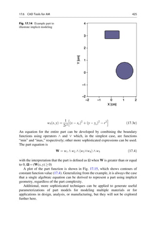
![17.7 Synthesis Methods
The capabilities of AM processes have inspired many people to try to design
structures so that they have minimum weight, without regard to geometric com-
plexity. Quite a few researchers are investigating methods for synthesizing light
weight structures, with the intention of fabricating the resulting structures using
AM. The work has been extended in some cases to the design of compliant
mechanisms, that is, one-piece structures that move. In this section, we provide a
brief survey of some recent research in this area. A brief exploration of optimization
methods will be covered, with an emphasis on the emerging area of topology
optimization that promises to aid designers in efficiently exploring novel structures.
17.7.1 Theoretically Optimal Lightweight Structures
Several years ago, researchers rediscovered the pioneering work of AGM Michell
in the early 1900s who developed the mathematical conditions under which struc-
ture weight becomes minimized [27]. He proved that structures can have minimum
weight if their members are purely tension-compression members (i.e., are trusses)
and derived the rules for truss layout. A typical Michell truss is shown in Fig. 17.16
for a common loaded plate structural problem. Note that the solution has a “wagon
wheel” structure.
Fig. 17.15 Contours of
implicit part equation
426 17 Design for Additive Manufacturing](https://image.slidesharecdn.com/1-230308091212-68402451/85/1-Additive-manufacturing-pdf-440-320.jpg)
![In general, it is difficult to compute optimal Michell truss layouts for any but the
simplest 2D cases. Some researchers have developed numerical procedures for
computing approximate solutions. At least one research group has proposed to
fabricate Michell trusses using AM processes and has investigated multiple mate-
rial solution cases [28]. For proposed synthesis algorithms for large complex
problems, Michell trusses provide an excellent baseline against which solutions
for more complicated problems can be compared.
17.7.2 Optimization Methods
In our context, optimization methods seek to improve the design of an artifact by
adjusting values of design variables in order to achieve desired objectives, typically
related to structural performance or weight, as well as possible without violating
constraints. A variety of optimization problem formulations has been developed
that vary based on type of objectives and scope of the problem. Good textbooks [29]
and many research papers have been written on the subject. The three main types of
optimization problems that have been explored for design for AM include, in order
of increasing complexity and scope:
• Size optimization—where values of dimensions are determined
• Shape optimization—where shapes of part surfaces are changed
• Topology optimization—where distributions of material are explored
In size optimization, the values of selected dimensions are determined that best
achieve the objectives while satisfying any constraints. For typical structural
optimization applications, objectives could include the minimization of maximum
stress, strain energy, deflection, or part volume or weight. One or more of these
quantities may also be modeled as constraints. For many mechanical parts, a small
number of size dimensions will be part of the optimization problem. However, for
cellular structures, such as lattices, the number of design variables could number in
the tens or hundreds of thousands.
Fig. 17.16 Michell truss layout (b) for simple loaded plate example (a)
17.7 Synthesis Methods 427](https://image.slidesharecdn.com/1-230308091212-68402451/85/1-Additive-manufacturing-pdf-441-320.jpg)
![Shape optimization is a generalization of size optimization. Typically the shape
of bounding curves or surfaces is optimized to achieve similar objectives and
constraints. As such, the positions of control vertices for curves or surfaces are
often used as the design variables. Shape and size optimization are frequently
combined in order to optimize structures that have free-form shapes, as well as
standard shapes (e.g., cylinders) with dimensions.
In topology optimization, the overall shape, arrangement of shape elements, and
connectivity of the design domain are determined. Again, part volume or compli-
ance is minimized, subject to constraints on, for example, volume, compliance,
stress, strain energy, and possibly additional considerations. The primary
differences between topology optimization and shape or size optimization are in
the starting geometric configuration and the choice of variables, which can lead to
very significant improvements in structural performance. The recent interest in
topology optimization as a design method for AM warrants a closer look into this
technology.
17.7.3 Topology Optimization
Topology optimization (TO) methods determine the overall configuration of shape
elements in a design problem. Often, TO results are used as inputs to subsequent
size or shape optimization problems. As structural optimization methods, finite
element analyses are performed typically during each iteration of the optimization
method, which means that TO can be computationally demanding. Furthermore,
TO solutions should result in structures that are nearly fully stressed, or have
constant strain energy, throughout the structure geometry based on the specified
loading conditions. Two main approaches have been developed for TO problems:
truss-based and volume-based density methods.
17.7.3.1 Truss-Based Methods
In the truss-based approach, a mesh of struts among a set of nodes is defined in a
volume of interest, where sometimes the mesh represents a complete graph (e.g.,
ground truss) and sometimes it is based on unit cells. Topology optimization
proceeds to identify which struts are most important for the problem, determine
their size (e.g., diameter), and remove struts with small sizes. Result quality is often
a strong function of the starting mesh of struts. Results will resemble the lattice
structures presented earlier, with variations in strut diameters evident.
In the first variations of truss-based methods, a ground truss was defined over a
grid of nodes, with each node connected to every other node by a truss element.
Each element’s diameter was used as the design variable. As optimization proceeds,
those elements whose diameters become small are deleted from the design.
Although the methods worked well, they tended to be computationally expensive.
Recently, more sophisticated methods have been developed that utilize a different
problem formulation, involving background meshes and analytical derivatives for
computation of sensitivities, for truss optimization methods [30]. Good results have
428 17 Design for Additive Manufacturing](https://image.slidesharecdn.com/1-230308091212-68402451/85/1-Additive-manufacturing-pdf-442-320.jpg)
![been achieved when both truss element size and position are used as design
variables. Variations of these approaches have demonstrated the capability of
achieving risk-based or reliability-related objectives [31].
Other synthesis methods utilize heuristic optimization methods in an attempt to
greatly reduce the number of design variables in the optimization problem. For
example, the Size Matching and Scaling (SMS) method starts with a conformal
lattice structure (Sect. 17.5.2) but only requires two design variables, the minimum
and maximum strut diameters, to optimize the structure [18]. The method works by
performing a finite element analysis (FEA) on a solid body of the design. A
conformal lattice structure is constructed that fits within the solid body. Local strain
or stress values from the FEA results are used to scale struts in the lattice structure
resulting in a set of relative strut size values. Size optimization is performed on the
lattice structure to determine the values of the minimum and maximum strut
diameters, using frame elements to model the lattice structure. Application of the
SMS method to a simplified UAV fuselage design problem is illustrated in
Fig. 17.17. Note that regions of high stress result in thick struts.
17.7.3.2 Volume-Based Density Methods
The second main approach is based on determining the appropriate material density
in a set of voxels that comprise a spatial domain. The density-based TO method that
is most common, and is used in the commercial software packages, is known as the
SIMP (Solid Isotropic Material with Penalization) method. The starting geometry
for the problem is a rectilinear block that is composed of a set of voxels. Each voxel
has a density value which is used as its design variable. A density value of
1 indicates that the material is fully dense, while a value of 0 indicates that no
material is present. Intermediate values indicate that the material need not be fully
solid to support the local stress state in that voxel. Solutions are preferred that have
voxels that are either fully dense or near 0 density, since typically partially dense
materials are difficult to manufacture. Density values are used to scale voxel
stiffness values in the FEA models that are used during the TO process.
The typical topology optimization problem is formulated as [32]:
Side View
Bottom View
a
b
Fig. 17.17 SMS method results on UAV fuselage design problem
17.7 Synthesis Methods 429](https://image.slidesharecdn.com/1-230308091212-68402451/85/1-Additive-manufacturing-pdf-443-320.jpg)