Digital image filtering method .

1. SPATIAL FILTERING

2. NEIGHBOURHOOD OPERATIONS
• simply operate on a larger neighbourhood of pixels than point
operations
• Neighbourhoods  mostly a rectangle around a central pixel
• Any size rectangle and any shape filter are possible
Origin x
y Image f (x, y)
(x, y)
Neighbourhood

3. NEIGHBOURHOOD OPERATIONS
• Some simple neighbourhood operations :
• Min: Set the pixel value to the minimum in the neighbourhood
• Max: Set the pixel value to the maximum in the neighbourhood
• Median: The median value of a set of numbers is the midpoint value in that
set (e.g. from the set [1, 7, 15, 18, 24] 15 is the median). Sometimes the
median works better than the average

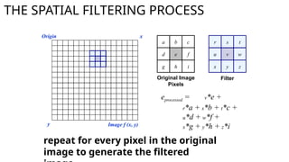
4. THE SPATIAL FILTERING PROCESS
r s t
u v w
x y z
Origin x
y Image f (x, y)
eprocessed = v*e +
r*a + s*b + t*c +
u*d + w*f +
x*g + y*h + z*i
Filter
a b c
d e f
g h i
Original Image
Pixels
repeat for every pixel in the original
image to generate the filtered

5. THE SPATIAL FILTERING
 

 




a
a
s
b
b
t
t
y
s
x
f
t
s
w
y
x
g )
,
(
)
,
(
)
,
(

6. THE SPATIAL FILTERING - SMOOTHING
One of the simplest spatial filtering operations we can
perform is a smoothing operation
– Simply average all of the pixels in a neighbourhood around a
central value
– Especially useful
in removing noise
from images
– Also useful for
highlighting
details
Simple
averaging
filter

7. THE SPATIAL FILTERING - SMOOTHING
1
/9
1
/9
1
/9
1
/9
1
/9
1
/9
1
/9
1
/9
1
/9
Image f (x, y)
e = 1
/9*106 +
1
/9*104 + 1
/9*100 + 1
/9*108 +
1
/9*99 + 1
/9*98 +
1
/9*95 + 1
/9*90 + 1
/9*85
= 98.3333
Filter
1
/9
1
/9
1
/9
1
/9
1
/9
1
/9
1
/9
1
/9
1
/9
104 100 108
99 106 98
95 90 85
Original Image
Pixels
*
Origin

8. Smoothing Example
The image at the top left
is an original image of
size 500*500 pixels
The subsequent images
show the image after
filtering with an averaging
filter of increasing sizes
– 3, 5, 9, 15 and 35
Notice how detail begins
to disappear

9. Weighted Smoothing Filters
More effective smoothing filters by allowing different
pixels in the neighbourhood different weights in the
averaging function
– Pixels closer to the
central pixel are more
important
– Often referred to as a
weighted averaging
Weighted
averaging filter
Distance =1
px
Distance =1.4 px

10. Weighted Smoothing Filters
More effective smoothing filters by allowing different
pixels in the neighbourhood different weights in the
averaging function
– Pixels closer to the
central pixel are more
important
– Often referred to as a
weighted averaging
Weighted
averaging filter
Distance =1
px
Distance =1.4 px

11. Weighted Smoothing Filters
Filtering is often used to remove noise from images
Sometimes a median filter works better than an averaging
filter
Original Image
With Noise
Image After
Averaging Filter
Image After
Median Filter
Still noisy

12. Filtering At The EDGES
At the edges of an image we are missing pixels to form a
neighbourhood
Origin x
y Image f (x, y)
e
e
e
e
e e
e
?

13. Filtering At The EDGES
Pad the image
Typically with either all white or all black pixels (ZERO PADDING)

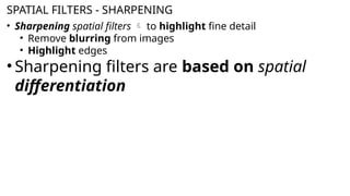
14. SPATIAL FILTERS - SHARPENING
• Sharpening spatial filters  to highlight fine detail
• Remove blurring from images
• Highlight edges
• Sharpening filters are based on spatial
differentiation

15. SPATIAL FILTERS - SHARPENING
• Differentiation measures the rate of change of a function
• It’s just the difference between subsequent values and
measures the rate of change of the function
• The formula for the 1st order derivative of a function is as
follows:
)
(
)
1
( x
f
x
f
x
f






16. SPATIAL FILTERS - SHARPENING
• The formula for the 2nd
order derivative of a function is
as follows:
•Simply takes into account the values
both before and after the current
value
)
(
2
)
1
(
)
1
(
2
2
x
f
x
f
x
f
x
f








17. SPATIAL FILTERS - SHARPENING
The 2nd
order derivative is more useful for image enhancement
than the 1st
derivative
Stronger response to fine detail
Simpler implementation
)
(
2
)
1
(
)
1
(
2
2
x
f
x
f
x
f
x
f








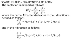
18. SPATIAL FILTERS – SHARPENING-LAPLACIAN
The Laplacian is defined as follows:
where the partial 2nd
order derivative in the x direction is
defined as follows:
and in the y direction as follows:
y
f
x
f
f 2
2
2
2
2







)
,
(
2
)
,
1
(
)
,
1
(
2
2
y
x
f
y
x
f
y
x
f
x
f







)
,
(
2
)
1
,
(
)
1
,
(
2
2
y
x
f
y
x
f
y
x
f
y
f








19. SPATIAL FILTERS – SHARPENING-LAPLACIAN
So, the Laplacian can be given as follows:
We can easily build a filter based on this:
? ? ?
? ? ?
? ? ?

20. SPATIAL FILTERS – SHARPENING-LAPLACIAN
So, the Laplacian can be given as follows:
We can easily build a filter based on this:
0 1 0
1 -4 1
0 1 0
f(x+1,y)
f(x+1,y-1)

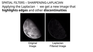
21. SPATIAL FILTERS – SHARPENING-LAPLACIAN
Applying the Laplacian  we get a new image that
highlights edges and other discontinuities

22. SPATIAL FILTERS – SHARPENING-LAPLACIAN
The result of a Laplacian filtering is not an enhanced image
Subtract the Laplacian result from the original image
to obtain a sharpened enhanced image
f
y
x
f
y
x
g 2
)
,
(
)
,
( 



23. SPATIAL FILTERS – SHARPENING-LAPLACIAN
f
y
x
f
y
x
g 2
)
,
(
)
,
( 


EDGES AND
DETAILS ARE MUCH
MORE OBVIOUS!

24. SPATIAL FILTERS – SHARPENING-LAPLACIAN
f
y
x
f
y
x
g 2
)
,
(
)
,
( 


EDGES AND
DETAILS ARE MUCH
MORE OBVIOUS!
ORIGINAL IMAGE
(blurry)
SHARPENED IMAGE BY
LAPLACIAN

25. SPATIAL FILTERS – SHARPENING-LAPLACIAN
• The entire enhancement  a single filtering operation

26. SPATIAL FILTERS – SHARPENING-LAPLACIAN
• The entire enhancement  a single filtering operation
0 -1 0
-1 5 -1
0 -1 0
A new filter that sharpens the image in one
step

27. 1st
ORDER DERIVATE OPERATORS - SOBEL
-1 0 1
-2 0 2
-1 0 1
EDGE DETECTION!
They are sensitive to noise in the
image, which can lead to false
edge detection.
•The positive values (+1
and +2) on the right
side give more weight
to pixels with higher
intensity, emphasizing
transitions from dark
to bright as we move
horizontally.
•Similarly, the negative
values (-1 and -2) on the
left side emphasize
transitions from
bright to dark.
-1 -2 -1
0 0 0
1 2 1

28. 1st
ORDER DERIVATE OPERATORS - SOBEL
Gy for the pixel in row 2, column 2 is 315.
Gx for the pixel in row 2, column 2 is 315.

29. 1st
ORDER DERIVATE OPERATORS - SOBEL
magnitude(G) =
magnitude(G) =
magnitude(G) ≈ 445

30. WHAT IF A PIXEL VALUE EXCEEDS 255?
445 0 255
200 0 0
210 155 255
=[(445-0)/(445-0)](255-0) + 0 = 255
255 0 146
115 0 0
120 89 146