Download to read offline
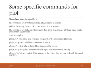
![Vectors
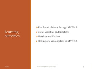
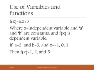
Vectors are classified as in two types:
Row vector: they are list of numbers separated by either commas or
spaces. The number of entries is known as the length of the vector and
the entries are often referred as “elements” or “components” of the
vector.
>>v=[1 3, sqrt(5)]
Column vector: to create a column vector type the left square bracket[
and then enter the element with a semicolon between them.
>>cv=[1; 2; 3; 4]
4/5/2016 DR. MOHAMMED DANISH/UNIKL-MICET 9](https://image.slidesharecdn.com/01-chaptermatlabintro-200405102204/85/01-Chapter-MATLAB-introduction-9-320.jpg)

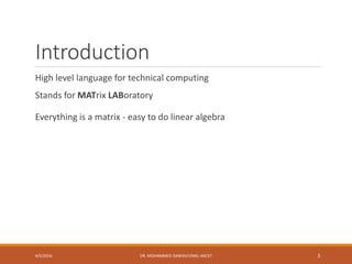
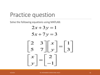
![Example plot
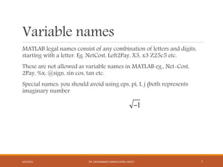
Year 1988 1989 1990 1991 1992 1993 1994
Sales
(millions)
8 12 20 22 18 24 27
To plot this data, the list of years is assigned to one vector (namely yr),
and the corresponding sales data is assigned to a second vector (named sle). The
command window where the vectors are created and the plot command is used is
shown below:
>> yr=[1988:1:1994];
>> sle=[8 12 20 22 18 24 27];
>> plot(yr,sle,'--r*','linewidth',2,'markersize',12)
4/5/2016 DR. MOHAMMED DANISH/UNIKL-MICET 15](https://image.slidesharecdn.com/01-chaptermatlabintro-200405102204/85/01-Chapter-MATLAB-introduction-15-320.jpg)


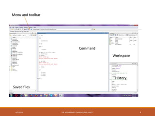
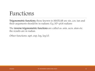
This document is a chapter on using MATLAB for problem solving. It discusses MATLAB's capabilities for simple calculations using variables and functions, working with matrices and vectors, plotting and visualization, and solving systems of linear equations. The chapter provides examples of MATLAB code for these tasks and concludes with a practice problem asking the reader to solve a system of equations using MATLAB.


![7.__Developing_a_Research_Proposal[1].pptx](https://cdn.slidesharecdn.com/ss_thumbnails/7-260131073037-df92dd7d-thumbnail.jpg?width=640&height=640&fit=bounds)


![Hacking-Uncovered-How-People-Get-Hacked-and-How-to-Stay-Safe[1].pptx](https://cdn.slidesharecdn.com/ss_thumbnails/hacking-uncovered-how-people-get-hacked-and-how-to-stay-safe1-260130170011-4883a9c7-thumbnail.jpg?width=640&height=640&fit=bounds)
![제 23회 보아즈(BOAZ) 빅데이터 컨퍼런스 - [MBOAX] : ABSA를 활용한 소비자 반응 분석 기반 운영 효율화 대시보드 설계](https://cdn.slidesharecdn.com/ss_thumbnails/3-1boaz23rdconferencemboax-260203102709-9d519923-thumbnail.jpg?width=640&height=640&fit=bounds)


