SlideShare a Scribd company logo
Question:

I need to do the following and have a problem figuring out what function to use
and how to use it: If Bob T is in 6 classes with 6 different grades in a room of 30
students with different first and last names and the names are put in aphbettical
order (Bobs name will not be in the same row each time) How would I only collect
the grades of Bob T? I have tried to use filter and dsum but failed given some
conditions. I really appreciate it if you can be of any help.


Answer:

It sounds like you need to use the VLOOKUP function.


Let's assume that the names of the students are found in Column A and the Grades in Column B.


In this case, you function will look like this:


=VLOOKUP("Bob T",$B1:$B100,2,FALSE)

With the vlookup formula, it doesn't matter on which row the data is.


This will retrieve the grade in one class. Adapt this formula for the rest of the classes and you should be
good to go.


Tags: VLOOKUP


Question:

how do I create a condition for date cells to change color when todays date is 30
days away from date in cell and past the date in the cell?

Answer:

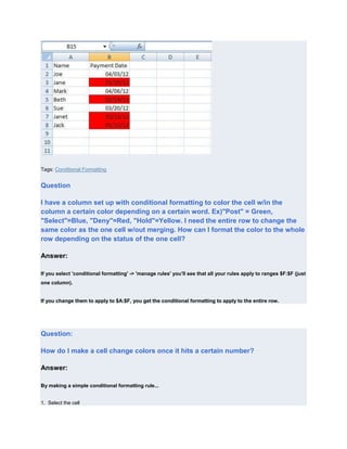
I assume your data looks something like this:
To highlight the cells that are 30 days or more before today's date, you should select cell B2 and use the
following conditional formatting rule:


Then, copy the rule to the other cells using the brush tool (format painter) and you will get this result:
Tags: Conditional Formatting


Question

I have a column set up with conditional formatting to color the cell w/in the
column a certain color depending on a certain word. Ex)"Post" = Green,
"Select"=Blue, "Deny"=Red, "Hold"=Yellow. I need the entire row to change the
same color as the one cell w/out merging. How can I format the color to the whole
row depending on the status of the one cell?

Answer:

If you select 'conditional formatting' -> 'manage rules' you'll see that all your rules apply to ranges $F:$F (just
one column).


If you change them to apply to $A:$F, you get the conditional formatting to apply to the entire row.


Question:

How do I make a cell change colors once it hits a certain number?

Answer:

By making a simple conditional formatting rule...


1. Select the cell
2. From the Home ribbon select 'Conditiional Formatting'


3. Then select 'Highlight Cell Rules'


4. Then select 'Greater than'


5. Then enter your number (minus one).


6. Select how you want to higlight the cell and...


7. Press OK


And you're good to go.


Tags: Conditional Formatting


Question:

how to rank value with name result? for example: I have player name in A1:A5,
score in B1:B5, and I want to have rank based on higher score with player name
on it.

Answer:

Put the following formula in cell C1


=RANK(B1,$B$1:$B$5)


Then copy the formula to cells C2:C5.


And finaly, sort the table on column C.


Tags: RANK


Question:

I have a list of state abbreviations and in the column next to it I need to have the
time zones that correspond. How can I have the time zone column prepopulate
after I enter the state abbreviation?

Answer:
You should use the VLOOKUP function.


The following image shows a list of state abbreviations and corresponding time zones.


The sheet automatically translates the state abbreviation in cell D4 to the time zone in E4 by using the
following VLOOKUP formula


=VLOOKUP(D4,$A$1:$B$17,2,FALSE)


Its important to note that the range the VLOOKUP function uses is an absolute reference. You almost always
need to use absolute reference when defining the lookup array because while the formula is likely to be
copied and the lookup value reference may change, the lookup array range almost never changes.


Tags: VLOOKUP


                                       Not what
                                  you're looking for?
Response time: 3 minutes


Question:

I have created a vlookup that when copied gives me different results than the
manually entered formula. When I manually enter the formula, it works perfect;
this is a document with 2000+ rows so manually entering the formula is not an
option. I have never encountered this before. Any suggestions?

Answer:

It sounds like a relative reference problem. This happens a lot with VLOOKUPs.


Your formula probably looks something like this:


=VLOOKUP(E2,A2:C9,2,FALSE)


If you copy this formula one cell down it will look like this:


=VLOOKUP(E3,A3:C10,2,FALSE)


Note that E2 changed to E3 which is good, you want the formula to lookup the value in the next row But...


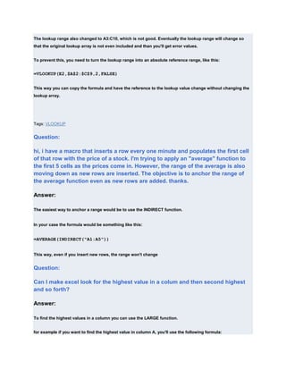
The lookup range also changed to A3:C10, which is not good. Eventually the lookup range will change so
that the original lookup array is not even included and than you'll get error values.


To prevent this, you need to turn the lookup range into an absolute reference range, like this:


=VLOOKUP(E2,$A$2:$C$9,2,FALSE)


This way you can copy the formula and have the reference to the lookup value change without changing the
lookup array.


Tags: VLOOKUP
Question:

I have 5 columns and 50000 rows, i want data from all 5 columns into the 6th
column in the format of SQL Insert query; e.g. insert into table1
values('a1','b1','c1', 'd1','e1') for the first row. and want to repeat the same for all
rows in the excel.

Answer:

Well this is a simple task of concatenating strings. The following formula will do the trick:


="Insert into table1 values('" & A1 & "','"& B1 & "','" & C1 & "','" & D1
& "','" & E1 & "')"

Once you have this formula in Cell F1, copy it to Cells F2:F50000 and the formula will automatically adjust to
create the right insert statements for you.


The Excel Power function


The power function is used (as you have probably guessed) to raise a number to a power.


For instance, the formula:


=Power(10,2) is 10*10 (can be written 102) which equals 100


=Power (2,3) is actually 2*2*2 (or 23), which equals 8

Note


Excel also includes the operator '^' for the Power() function.


So instead of writing:


=Power(10,2)


You can write:


=10^2
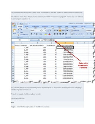
The power function can be used in many ways, but perhaps it's most well known use is with compound interest rate.


The following sheet shows the return on investment on a $5000 investment carrying a 5% interest rate over different
investment periods (column C).


You calculate the return on investment by raising the interest rate by the power of the time period then multiplying it
with the original investment sum.


This will translate to the following Excel formula:


=A2*POWER(B2,C2)


Note


To get a feel of the Power() function try the following exercise:
Open a new sheet and simulate the growth rate of an imaginary virus. The rules of the game are very simple. Each
generation the virus splits into 2 new viruses.


Put the number 2 in cell A1


Put the number of generations (start with 5) in cell A2


And put the formula =Power(A1,A2) in B2


B2 will show you how many viruses there are after 5 generations.


Now play with the number of generations and see how the results change.


Excel ROUNDUP, ROUNDDOWN and ROUND functions


In the previous example we calculated the return on investment by using the power function. If you look at the results
of the calculation on column D, you'll see that they show 5 digits after the decimal point.
While showing numbers after the decimal point is certainly more precise, it also makes reading the sheet much
harder because of all those extra numbers.


One of the ways to eliminate (or reduce) the digits after the decimal point is to use the ROUNDUP(), ROUNDDOWN()
and ROUND() functions.


As you probably gathered from its name, the ROUNDUP() function will round any given number up to the next round
number.


What's interesting is that ROUNDUP() also lets round up to a specific number of decimal points. That's done by
passing the number of decimal points you want to round up to as the second parameter (0 meaning to round up to
the closest whole number, 1 meaning there will be one digit after the decimal point, and so on).


For Example:


=ROUNDUP(18.23,0) will return 19
While


=ROUNDUP(18.23,1) will return 18.3


The ROUNDDOWN() acts exactly the same way as the ROUNDUP() function except it will round the number down to
the previous round number (with a specified number of digits).


For Example:


=ROUNDDOWN(18.23,0) will return 18


And


=ROUNDDOWN(18.23,1) will return 18.2


The ROUND() function will round to the closest number (given a specific number of digits).


For example:


=ROUND(18.23,0) will return 18


While


=ROUND(18.51,0) will return 19


Note


What do you think will the function =ROUND(18.5,0) return?


Will it return 19 or will it return 18?


Open Excel and check if your answer was correct.


Excel CEILING and FLOOR functions


The FLOOR() and CEILING() function are similar to the ROUND functions but serve a slightly different purpose.
The CEILING function receives two parameters (let's call them A and B) and returns the multiple of B that's both
closest to and larger than A.


For instance


=CEILING(10,3)


Will return 12 since 12 is the closest multiple of 3 which is also larger than 10.


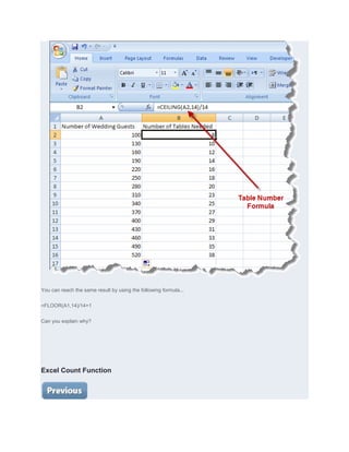
Imagine you wanted to calculate how many tables you should arrange for your wedding.


You know how many people you plan to invite to the wedding. And you know that each table seats 14 people.


The following formula will reveal the answer in a blink:


=CEILING(A1,14)/14


Enter the number of invitees into cell A1 and you've got your answer.
You can reach the same result by using the following formula...


=FLOOR(A1,14)/14+1


Can you explain why?


Excel Count Function
Counting is one of the things Excel does best. And if you probe the help files you'll find 5 different counting functions.


But let's turn to the basic COUNT() function.


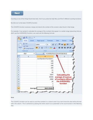
The COUNT() function receives a range and returns the number of the numeric value found in that range.


For example, if we wanted to calculate the average of the numbers that appear in a certain range (assuming that we
didn't use the AVERAGE() function), we could use the following formula:


Note


The COUNT() function can be used to count the numbers in a column even if you don't know the what will be the last
cell in the column. This is achieved by passing the entire column as a parameter to the count function in the following
way:
=COUNT(A:A)


I need to create a formula that shows when a value from a drop down list is
selected it will pre-populate in other cells information from another list

Answer:

You'll need to use the VLOOKUP function. In the following screen shot you can see that the Job field is auto-
filled after the name of the employee is selected form the drop down list.


This is the formula used to achieve this:


=VLOOKUP(B10,B3:C7,2,FALSE)

Question:

I need to do the following and have a problem figuring out what function to use
and how to use it: If Bob T is in 6 classes with 6 different grades in a room of 30
students with different first and last names and the names are put in aphbettical
order (Bobs name will not be in the same row each time) How would I only collect
the grades of Bob T? I have tried to use filter and dsum but failed given some
conditions. I really appreciate it if you can be of any help.


Answer:

It sounds like you need to use the VLOOKUP function.


Let's assume that the names of the students are found in Column A and the Grades in Column B.


In this case, you function will look like this:


=VLOOKUP("Bob T",$B1:$B100,2,FALSE)

With the vlookup formula, it doesn't matter on which row the data is.


This will retrieve the grade in one class. Adapt this formula for the rest of the classes and you should be
good to go.


Tags: VLOOKUP


Question:

I'm trying to work out percentage increases but when one of the cells has 0 in it
its giving me DIV/0 error How do i stop this?

Answer:

To avoid showing the DIV/0 error you should use the ISERROR() function like this:


=IF(ISERROR(A1/B1),"",A1/B1)


The function above will an empty value when the division formula returns an error.


Tags: IF ISERROR
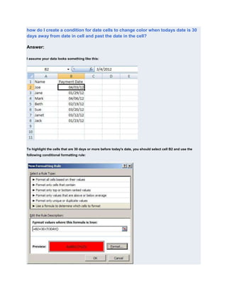
how do I create a condition for date cells to change color when todays date is 30
days away from date in cell and past the date in the cell?

Answer:

I assume your data looks something like this:


To highlight the cells that are 30 days or more before today's date, you should select cell B2 and use the
following conditional formatting rule:
Then, copy the rule to the other cells using the brush tool (format painter) and you will get this result:


Question:

I would like to have my data in excel automatically sort every time I open it to the
preference I have pre-set. I would rather this instead of always having to select
my data, hit data, sort, and etc. How would I do this?

Answer:

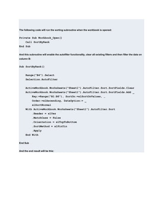
This can be done by using a VBA macro. For example, if you have the following data:
The following code will run the sorting subroutine when the workbook is opened:


Private Sub Workbook_Open()
      Call SortByRank
End Sub


And this subroutine will enable the autofilter functionality, clear all existing filters and then filter the data on
column B:


Sub SortByRank()


      Range("B4").Select
      Selection.AutoFilter


      ActiveWorkbook.Worksheets("Sheet1").AutoFilter.Sort.SortFields.Clear
      ActiveWorkbook.Worksheets("Sheet1").AutoFilter.Sort.SortFields.Add _
            Key:=Range("B1:B6"), SortOn:=xlSortOnValues, _
            Order:=xlAscending, DataOption:= _
            xlSortNormal
      With ActiveWorkbook.Worksheets("Sheet1").AutoFilter.Sort
            .Header = xlYes
            .MatchCase = False
            .Orientation = xlTopToBottom
            .SortMethod = xlPinYin
            .Apply
      End With


End Sub


And the end result will be this:
Tags: VBA


Question:

I have created a vlookup that when copied gives me different results than the
manually entered formula. When I manually enter the formula, it works perfect;
this is a document with 2000+ rows so manually entering the formula is not an
option. I have never encountered this before. Any suggestions?

Answer:

It sounds like a relative reference problem. This happens a lot with VLOOKUPs.


Your formula probably looks something like this:


=VLOOKUP(E2,A2:C9,2,FALSE)


If you copy this formula one cell down it will look like this:


=VLOOKUP(E3,A3:C10,2,FALSE)


Note that E2 changed to E3 which is good, you want the formula to lookup the value in the next row But...
The lookup range also changed to A3:C10, which is not good. Eventually the lookup range will change so
that the original lookup array is not even included and than you'll get error values.


To prevent this, you need to turn the lookup range into an absolute reference range, like this:


=VLOOKUP(E2,$A$2:$C$9,2,FALSE)


This way you can copy the formula and have the reference to the lookup value change without changing the
lookup array.


Tags: VLOOKUP


Question:

hi, i have a macro that inserts a row every one minute and populates the first cell
of that row with the price of a stock. I'm trying to apply an "average" function to
the first 5 cells as the prices come in. However, the range of the average is also
moving down as new rows are inserted. The objective is to anchor the range of
the average function even as new rows are added. thanks.

Answer:

The easiest way to anchor a range would be to use the INDIRECT function.


In your case the formula would be something like this:


=AVERAGE(INDIRECT("A1:A5"))


This way, even if you insert new rows, the range won't change


Question:

Can I make excel look for the highest value in a colum and then second highest
and so forth?

Answer:

To find the highest values in a column you can use the LARGE function.


for example if you want to find the highest value in column A, you'll use the following formula:
=LARGE(A:A,1)

To find the second highest value, just change the 1 in the previous formula to 2., like so:


=LARGE(A:A,2)


Tags: LARGE


Question:

How do I sum cells greater than a value even if there is a zero cell in between two
cells greater than the value.

Answer:

To sum cells that are greater than a value you should use the SUMIF() function.


For example, the following formula will sum all the values that are greater than 100 on column A


=SUMIF(A:A,">100")


And it doesn't matter if there is a cell that contains zero or any other value in that range.


Tags: SUMIF


I am trying to extract out a name within a cell. For example: 613490 Chong
Susanna,5087321900 In the above cell, I want to pull out just the name.

Answer:

Luckily, your string contains a space before the name and a comma after it. This makes it easy to find where
the name starts and it's length so you can 'cut' it out with the MID() function.


The following formula will extract the name for you:


=MID(A1,FIND(" ",A1)+1,FIND(",",A1)-FIND(" ",A1)-1)

Tags: MID FIND


How can I average cells but only ones with numbers greater than 0?

Answer:
By using the AVERAGEIF function


The following formula will return the average of all the cells that are bigger than 0 in range A1:A7 :


=AVERAGEIF(A1:A7,">0")

More Related Content

What's hot

Types of functions 05272011
Types of functions 05272011Types of functions 05272011
Types of functions 05272011
Boyet Aluan
 
Ch01 se
Ch01 seCh01 se
Ch01 se
parulian
 
Algebraic functions powerpoint
Algebraic functions powerpointAlgebraic functions powerpoint
Algebraic functions powerpoint
Caron White
 
Unit 3.1
Unit 3.1Unit 3.1
Unit 3.1
Mark Ryder
 
Maths iii quick review by Dr Asish K Mukhopadhyay
Maths iii quick review by Dr Asish K MukhopadhyayMaths iii quick review by Dr Asish K Mukhopadhyay
Maths iii quick review by Dr Asish K Mukhopadhyay
Dr. Asish K Mukhopadhyay
 
Goldie chapter 4 function
Goldie chapter 4 functionGoldie chapter 4 function
Goldie chapter 4 function
Sarah Sue Calbio
 
Unit 2.6
Unit 2.6Unit 2.6
Unit 2.6
Mark Ryder
 
bisection method
bisection methodbisection method
bisection method
Muhammad Usama
 
Nams- Roots of equations by numerical methods
Nams- Roots of equations by numerical methodsNams- Roots of equations by numerical methods
Nams- Roots of equations by numerical methods
Ruchi Maurya
 
An Introduction To Array Functions
An Introduction To Array FunctionsAn Introduction To Array Functions
An Introduction To Array Functions
posterro
 
Ch06 se
Ch06 seCh06 se
Ch06 se
parulian
 
Python Programming
Python Programming Python Programming
Python Programming
Sreedhar Chowdam
 
Finding All Real Zeros Of A Polynomial With Examples
Finding All Real Zeros Of A Polynomial With ExamplesFinding All Real Zeros Of A Polynomial With Examples
Finding All Real Zeros Of A Polynomial With Examples
Kristen T
 
Inroduction
InroductionInroduction
Inroduction
Phoebe Ann Marco
 
Unit 2.3
Unit 2.3Unit 2.3
Unit 2.3
Mark Ryder
 
6.3 evaluating-and-graphing-polynomila-functions
6.3 evaluating-and-graphing-polynomila-functions6.3 evaluating-and-graphing-polynomila-functions
6.3 evaluating-and-graphing-polynomila-functions
morrobea
 
Unit .3
Unit .3Unit .3
Unit .3
Mark Ryder
 
Function notation by sadiq
Function notation by sadiqFunction notation by sadiq
Function notation by sadiq
Sadiq Hussain
 
03 Chapter MATLAB finite precision arithmatic
03 Chapter MATLAB finite precision arithmatic03 Chapter MATLAB finite precision arithmatic
03 Chapter MATLAB finite precision arithmatic
Dr. Mohammed Danish
 

What's hot (19)

Types of functions 05272011
Types of functions 05272011Types of functions 05272011
Types of functions 05272011
 
Ch01 se
Ch01 seCh01 se
Ch01 se
 
Algebraic functions powerpoint
Algebraic functions powerpointAlgebraic functions powerpoint
Algebraic functions powerpoint
 
Unit 3.1
Unit 3.1Unit 3.1
Unit 3.1
 
Maths iii quick review by Dr Asish K Mukhopadhyay
Maths iii quick review by Dr Asish K MukhopadhyayMaths iii quick review by Dr Asish K Mukhopadhyay
Maths iii quick review by Dr Asish K Mukhopadhyay
 
Goldie chapter 4 function
Goldie chapter 4 functionGoldie chapter 4 function
Goldie chapter 4 function
 
Unit 2.6
Unit 2.6Unit 2.6
Unit 2.6
 
bisection method
bisection methodbisection method
bisection method
 
Nams- Roots of equations by numerical methods
Nams- Roots of equations by numerical methodsNams- Roots of equations by numerical methods
Nams- Roots of equations by numerical methods
 
An Introduction To Array Functions
An Introduction To Array FunctionsAn Introduction To Array Functions
An Introduction To Array Functions
 
Ch06 se
Ch06 seCh06 se
Ch06 se
 
Python Programming
Python Programming Python Programming
Python Programming
 
Finding All Real Zeros Of A Polynomial With Examples
Finding All Real Zeros Of A Polynomial With ExamplesFinding All Real Zeros Of A Polynomial With Examples
Finding All Real Zeros Of A Polynomial With Examples
 
Inroduction
InroductionInroduction
Inroduction
 
Unit 2.3
Unit 2.3Unit 2.3
Unit 2.3
 
6.3 evaluating-and-graphing-polynomila-functions
6.3 evaluating-and-graphing-polynomila-functions6.3 evaluating-and-graphing-polynomila-functions
6.3 evaluating-and-graphing-polynomila-functions
 
Unit .3
Unit .3Unit .3
Unit .3
 
Function notation by sadiq
Function notation by sadiqFunction notation by sadiq
Function notation by sadiq
 
03 Chapter MATLAB finite precision arithmatic
03 Chapter MATLAB finite precision arithmatic03 Chapter MATLAB finite precision arithmatic
03 Chapter MATLAB finite precision arithmatic
 

Similar to Excel formulas

Ms excel commands
Ms excel commandsMs excel commands
Ms excel commands
DiyaVerma14
 
Top 20 microsoft excel formulas you must know
Top 20 microsoft excel formulas you must knowTop 20 microsoft excel formulas you must know
Top 20 microsoft excel formulas you must know
AlexHenderson59
 
Libre Office Calc Lesson 4: Understanding Functions
Libre Office Calc Lesson 4: Understanding FunctionsLibre Office Calc Lesson 4: Understanding Functions
Libre Office Calc Lesson 4: Understanding Functions
Smart Chicago Collaborative
 
Excel basics for everyday use-the more advanced stuff
Excel basics for everyday use-the more advanced stuffExcel basics for everyday use-the more advanced stuff
Excel basics for everyday use-the more advanced stuff
Kevin McLogan
 
Excel Function Training
Excel Function TrainingExcel Function Training
Excel Function Training
kapileshwar kumar
 
Excel basics for everyday use part three
Excel basics for everyday use part threeExcel basics for everyday use part three
Excel basics for everyday use part three
Kevin McLogan
 
Introduction to micro soft Training ms Excel.ppt
Introduction to micro soft Training ms Excel.pptIntroduction to micro soft Training ms Excel.ppt
Introduction to micro soft Training ms Excel.ppt
dejene3
 
In Section 1 on the Data page, complete each column of the spreads.docx
In Section 1 on the Data page, complete each column of the spreads.docxIn Section 1 on the Data page, complete each column of the spreads.docx
In Section 1 on the Data page, complete each column of the spreads.docx
sleeperharwell
 
Excel formula
Excel formulaExcel formula
Manual for Troubleshooting Formulas & Functions in Excel
Manual for Troubleshooting Formulas & Functions in ExcelManual for Troubleshooting Formulas & Functions in Excel
Manual for Troubleshooting Formulas & Functions in Excel
Christopher Ward
 
Excel.useful fns
Excel.useful fnsExcel.useful fns
Excel.useful fns
Rahul Singhal
 
Excel training
Excel trainingExcel training
Excel training
Alexandru Gologan
 
cheatsheet from DataCamp.pdf
cheatsheet from DataCamp.pdfcheatsheet from DataCamp.pdf
cheatsheet from DataCamp.pdf
Rakesh Nimhan
 
Get more from excel
Get more from excelGet more from excel
Get more from excel
Gopal Sridharan
 
Creating Formulas in Excel
Creating Formulas in ExcelCreating Formulas in Excel
Creating Formulas in Excel
Kim Estes
 
Excel 2007- Enter Formulas
Excel 2007- Enter FormulasExcel 2007- Enter Formulas
Excel 2007- Enter Formulas
Oklahoma Dept. Mental Health
 
3 inner plumbing Excel tips
3 inner plumbing Excel tips3 inner plumbing Excel tips
3 inner plumbing Excel tips
Martin van Wunnik
 
Excell%20basic%20training(3) 143
Excell%20basic%20training(3) 143Excell%20basic%20training(3) 143
Excell%20basic%20training(3) 143
Ramesh Meti
 
Microsoft Excel Advanced Features
Microsoft Excel Advanced FeaturesMicrosoft Excel Advanced Features
Microsoft Excel Advanced Features
AkashMeghwar2
 
Functions and formulas of ms excel
Functions and formulas of ms excelFunctions and formulas of ms excel
Functions and formulas of ms excel
madhuparna bhowmik
 

Similar to Excel formulas (20)

Ms excel commands
Ms excel commandsMs excel commands
Ms excel commands
 
Top 20 microsoft excel formulas you must know
Top 20 microsoft excel formulas you must knowTop 20 microsoft excel formulas you must know
Top 20 microsoft excel formulas you must know
 
Libre Office Calc Lesson 4: Understanding Functions
Libre Office Calc Lesson 4: Understanding FunctionsLibre Office Calc Lesson 4: Understanding Functions
Libre Office Calc Lesson 4: Understanding Functions
 
Excel basics for everyday use-the more advanced stuff
Excel basics for everyday use-the more advanced stuffExcel basics for everyday use-the more advanced stuff
Excel basics for everyday use-the more advanced stuff
 
Excel Function Training
Excel Function TrainingExcel Function Training
Excel Function Training
 
Excel basics for everyday use part three
Excel basics for everyday use part threeExcel basics for everyday use part three
Excel basics for everyday use part three
 
Introduction to micro soft Training ms Excel.ppt
Introduction to micro soft Training ms Excel.pptIntroduction to micro soft Training ms Excel.ppt
Introduction to micro soft Training ms Excel.ppt
 
In Section 1 on the Data page, complete each column of the spreads.docx
In Section 1 on the Data page, complete each column of the spreads.docxIn Section 1 on the Data page, complete each column of the spreads.docx
In Section 1 on the Data page, complete each column of the spreads.docx
 
Excel formula
Excel formulaExcel formula
Excel formula
 
Manual for Troubleshooting Formulas & Functions in Excel
Manual for Troubleshooting Formulas & Functions in ExcelManual for Troubleshooting Formulas & Functions in Excel
Manual for Troubleshooting Formulas & Functions in Excel
 
Excel.useful fns
Excel.useful fnsExcel.useful fns
Excel.useful fns
 
Excel training
Excel trainingExcel training
Excel training
 
cheatsheet from DataCamp.pdf
cheatsheet from DataCamp.pdfcheatsheet from DataCamp.pdf
cheatsheet from DataCamp.pdf
 
Get more from excel
Get more from excelGet more from excel
Get more from excel
 
Creating Formulas in Excel
Creating Formulas in ExcelCreating Formulas in Excel
Creating Formulas in Excel
 
Excel 2007- Enter Formulas
Excel 2007- Enter FormulasExcel 2007- Enter Formulas
Excel 2007- Enter Formulas
 
3 inner plumbing Excel tips
3 inner plumbing Excel tips3 inner plumbing Excel tips
3 inner plumbing Excel tips
 
Excell%20basic%20training(3) 143
Excell%20basic%20training(3) 143Excell%20basic%20training(3) 143
Excell%20basic%20training(3) 143
 
Microsoft Excel Advanced Features
Microsoft Excel Advanced FeaturesMicrosoft Excel Advanced Features
Microsoft Excel Advanced Features
 
Functions and formulas of ms excel
Functions and formulas of ms excelFunctions and formulas of ms excel
Functions and formulas of ms excel
 

Excel formulas

  • 1. Question: I need to do the following and have a problem figuring out what function to use and how to use it: If Bob T is in 6 classes with 6 different grades in a room of 30 students with different first and last names and the names are put in aphbettical order (Bobs name will not be in the same row each time) How would I only collect the grades of Bob T? I have tried to use filter and dsum but failed given some conditions. I really appreciate it if you can be of any help. Answer: It sounds like you need to use the VLOOKUP function. Let's assume that the names of the students are found in Column A and the Grades in Column B. In this case, you function will look like this: =VLOOKUP("Bob T",$B1:$B100,2,FALSE) With the vlookup formula, it doesn't matter on which row the data is. This will retrieve the grade in one class. Adapt this formula for the rest of the classes and you should be good to go. Tags: VLOOKUP Question: how do I create a condition for date cells to change color when todays date is 30 days away from date in cell and past the date in the cell? Answer: I assume your data looks something like this:
  • 2. To highlight the cells that are 30 days or more before today's date, you should select cell B2 and use the following conditional formatting rule: Then, copy the rule to the other cells using the brush tool (format painter) and you will get this result:
  • 3. Tags: Conditional Formatting Question I have a column set up with conditional formatting to color the cell w/in the column a certain color depending on a certain word. Ex)"Post" = Green, "Select"=Blue, "Deny"=Red, "Hold"=Yellow. I need the entire row to change the same color as the one cell w/out merging. How can I format the color to the whole row depending on the status of the one cell? Answer: If you select 'conditional formatting' -> 'manage rules' you'll see that all your rules apply to ranges $F:$F (just one column). If you change them to apply to $A:$F, you get the conditional formatting to apply to the entire row. Question: How do I make a cell change colors once it hits a certain number? Answer: By making a simple conditional formatting rule... 1. Select the cell
  • 4. 2. From the Home ribbon select 'Conditiional Formatting' 3. Then select 'Highlight Cell Rules' 4. Then select 'Greater than' 5. Then enter your number (minus one). 6. Select how you want to higlight the cell and... 7. Press OK And you're good to go. Tags: Conditional Formatting Question: how to rank value with name result? for example: I have player name in A1:A5, score in B1:B5, and I want to have rank based on higher score with player name on it. Answer: Put the following formula in cell C1 =RANK(B1,$B$1:$B$5) Then copy the formula to cells C2:C5. And finaly, sort the table on column C. Tags: RANK Question: I have a list of state abbreviations and in the column next to it I need to have the time zones that correspond. How can I have the time zone column prepopulate after I enter the state abbreviation? Answer:
  • 5. You should use the VLOOKUP function. The following image shows a list of state abbreviations and corresponding time zones. The sheet automatically translates the state abbreviation in cell D4 to the time zone in E4 by using the following VLOOKUP formula =VLOOKUP(D4,$A$1:$B$17,2,FALSE) Its important to note that the range the VLOOKUP function uses is an absolute reference. You almost always need to use absolute reference when defining the lookup array because while the formula is likely to be copied and the lookup value reference may change, the lookup array range almost never changes. Tags: VLOOKUP Not what you're looking for?
  • 6. Response time: 3 minutes Question: I have created a vlookup that when copied gives me different results than the manually entered formula. When I manually enter the formula, it works perfect; this is a document with 2000+ rows so manually entering the formula is not an option. I have never encountered this before. Any suggestions? Answer: It sounds like a relative reference problem. This happens a lot with VLOOKUPs. Your formula probably looks something like this: =VLOOKUP(E2,A2:C9,2,FALSE) If you copy this formula one cell down it will look like this: =VLOOKUP(E3,A3:C10,2,FALSE) Note that E2 changed to E3 which is good, you want the formula to lookup the value in the next row But... The lookup range also changed to A3:C10, which is not good. Eventually the lookup range will change so that the original lookup array is not even included and than you'll get error values. To prevent this, you need to turn the lookup range into an absolute reference range, like this: =VLOOKUP(E2,$A$2:$C$9,2,FALSE) This way you can copy the formula and have the reference to the lookup value change without changing the lookup array. Tags: VLOOKUP
  • 7. Question: I have 5 columns and 50000 rows, i want data from all 5 columns into the 6th column in the format of SQL Insert query; e.g. insert into table1 values('a1','b1','c1', 'd1','e1') for the first row. and want to repeat the same for all rows in the excel. Answer: Well this is a simple task of concatenating strings. The following formula will do the trick: ="Insert into table1 values('" & A1 & "','"& B1 & "','" & C1 & "','" & D1 & "','" & E1 & "')" Once you have this formula in Cell F1, copy it to Cells F2:F50000 and the formula will automatically adjust to create the right insert statements for you. The Excel Power function The power function is used (as you have probably guessed) to raise a number to a power. For instance, the formula: =Power(10,2) is 10*10 (can be written 102) which equals 100 =Power (2,3) is actually 2*2*2 (or 23), which equals 8 Note Excel also includes the operator '^' for the Power() function. So instead of writing: =Power(10,2) You can write: =10^2
  • 8. The power function can be used in many ways, but perhaps it's most well known use is with compound interest rate. The following sheet shows the return on investment on a $5000 investment carrying a 5% interest rate over different investment periods (column C). You calculate the return on investment by raising the interest rate by the power of the time period then multiplying it with the original investment sum. This will translate to the following Excel formula: =A2*POWER(B2,C2) Note To get a feel of the Power() function try the following exercise:
  • 9. Open a new sheet and simulate the growth rate of an imaginary virus. The rules of the game are very simple. Each generation the virus splits into 2 new viruses. Put the number 2 in cell A1 Put the number of generations (start with 5) in cell A2 And put the formula =Power(A1,A2) in B2 B2 will show you how many viruses there are after 5 generations. Now play with the number of generations and see how the results change. Excel ROUNDUP, ROUNDDOWN and ROUND functions In the previous example we calculated the return on investment by using the power function. If you look at the results of the calculation on column D, you'll see that they show 5 digits after the decimal point.
  • 10. While showing numbers after the decimal point is certainly more precise, it also makes reading the sheet much harder because of all those extra numbers. One of the ways to eliminate (or reduce) the digits after the decimal point is to use the ROUNDUP(), ROUNDDOWN() and ROUND() functions. As you probably gathered from its name, the ROUNDUP() function will round any given number up to the next round number. What's interesting is that ROUNDUP() also lets round up to a specific number of decimal points. That's done by passing the number of decimal points you want to round up to as the second parameter (0 meaning to round up to the closest whole number, 1 meaning there will be one digit after the decimal point, and so on). For Example: =ROUNDUP(18.23,0) will return 19
  • 11. While =ROUNDUP(18.23,1) will return 18.3 The ROUNDDOWN() acts exactly the same way as the ROUNDUP() function except it will round the number down to the previous round number (with a specified number of digits). For Example: =ROUNDDOWN(18.23,0) will return 18 And =ROUNDDOWN(18.23,1) will return 18.2 The ROUND() function will round to the closest number (given a specific number of digits). For example: =ROUND(18.23,0) will return 18 While =ROUND(18.51,0) will return 19 Note What do you think will the function =ROUND(18.5,0) return? Will it return 19 or will it return 18? Open Excel and check if your answer was correct. Excel CEILING and FLOOR functions The FLOOR() and CEILING() function are similar to the ROUND functions but serve a slightly different purpose.
  • 12. The CEILING function receives two parameters (let's call them A and B) and returns the multiple of B that's both closest to and larger than A. For instance =CEILING(10,3) Will return 12 since 12 is the closest multiple of 3 which is also larger than 10. Imagine you wanted to calculate how many tables you should arrange for your wedding. You know how many people you plan to invite to the wedding. And you know that each table seats 14 people. The following formula will reveal the answer in a blink: =CEILING(A1,14)/14 Enter the number of invitees into cell A1 and you've got your answer.
  • 13. You can reach the same result by using the following formula... =FLOOR(A1,14)/14+1 Can you explain why? Excel Count Function
  • 14. Counting is one of the things Excel does best. And if you probe the help files you'll find 5 different counting functions. But let's turn to the basic COUNT() function. The COUNT() function receives a range and returns the number of the numeric value found in that range. For example, if we wanted to calculate the average of the numbers that appear in a certain range (assuming that we didn't use the AVERAGE() function), we could use the following formula: Note The COUNT() function can be used to count the numbers in a column even if you don't know the what will be the last cell in the column. This is achieved by passing the entire column as a parameter to the count function in the following way:
  • 15. =COUNT(A:A) I need to create a formula that shows when a value from a drop down list is selected it will pre-populate in other cells information from another list Answer: You'll need to use the VLOOKUP function. In the following screen shot you can see that the Job field is auto- filled after the name of the employee is selected form the drop down list. This is the formula used to achieve this: =VLOOKUP(B10,B3:C7,2,FALSE) Question: I need to do the following and have a problem figuring out what function to use and how to use it: If Bob T is in 6 classes with 6 different grades in a room of 30 students with different first and last names and the names are put in aphbettical order (Bobs name will not be in the same row each time) How would I only collect
  • 16. the grades of Bob T? I have tried to use filter and dsum but failed given some conditions. I really appreciate it if you can be of any help. Answer: It sounds like you need to use the VLOOKUP function. Let's assume that the names of the students are found in Column A and the Grades in Column B. In this case, you function will look like this: =VLOOKUP("Bob T",$B1:$B100,2,FALSE) With the vlookup formula, it doesn't matter on which row the data is. This will retrieve the grade in one class. Adapt this formula for the rest of the classes and you should be good to go. Tags: VLOOKUP Question: I'm trying to work out percentage increases but when one of the cells has 0 in it its giving me DIV/0 error How do i stop this? Answer: To avoid showing the DIV/0 error you should use the ISERROR() function like this: =IF(ISERROR(A1/B1),"",A1/B1) The function above will an empty value when the division formula returns an error. Tags: IF ISERROR
  • 17. how do I create a condition for date cells to change color when todays date is 30 days away from date in cell and past the date in the cell? Answer: I assume your data looks something like this: To highlight the cells that are 30 days or more before today's date, you should select cell B2 and use the following conditional formatting rule:
  • 18. Then, copy the rule to the other cells using the brush tool (format painter) and you will get this result: Question: I would like to have my data in excel automatically sort every time I open it to the preference I have pre-set. I would rather this instead of always having to select my data, hit data, sort, and etc. How would I do this? Answer: This can be done by using a VBA macro. For example, if you have the following data:
  • 19. The following code will run the sorting subroutine when the workbook is opened: Private Sub Workbook_Open() Call SortByRank End Sub And this subroutine will enable the autofilter functionality, clear all existing filters and then filter the data on column B: Sub SortByRank() Range("B4").Select Selection.AutoFilter ActiveWorkbook.Worksheets("Sheet1").AutoFilter.Sort.SortFields.Clear ActiveWorkbook.Worksheets("Sheet1").AutoFilter.Sort.SortFields.Add _ Key:=Range("B1:B6"), SortOn:=xlSortOnValues, _ Order:=xlAscending, DataOption:= _ xlSortNormal With ActiveWorkbook.Worksheets("Sheet1").AutoFilter.Sort .Header = xlYes .MatchCase = False .Orientation = xlTopToBottom .SortMethod = xlPinYin .Apply End With End Sub And the end result will be this:
  • 20. Tags: VBA Question: I have created a vlookup that when copied gives me different results than the manually entered formula. When I manually enter the formula, it works perfect; this is a document with 2000+ rows so manually entering the formula is not an option. I have never encountered this before. Any suggestions? Answer: It sounds like a relative reference problem. This happens a lot with VLOOKUPs. Your formula probably looks something like this: =VLOOKUP(E2,A2:C9,2,FALSE) If you copy this formula one cell down it will look like this: =VLOOKUP(E3,A3:C10,2,FALSE) Note that E2 changed to E3 which is good, you want the formula to lookup the value in the next row But...
  • 21. The lookup range also changed to A3:C10, which is not good. Eventually the lookup range will change so that the original lookup array is not even included and than you'll get error values. To prevent this, you need to turn the lookup range into an absolute reference range, like this: =VLOOKUP(E2,$A$2:$C$9,2,FALSE) This way you can copy the formula and have the reference to the lookup value change without changing the lookup array. Tags: VLOOKUP Question: hi, i have a macro that inserts a row every one minute and populates the first cell of that row with the price of a stock. I'm trying to apply an "average" function to the first 5 cells as the prices come in. However, the range of the average is also moving down as new rows are inserted. The objective is to anchor the range of the average function even as new rows are added. thanks. Answer: The easiest way to anchor a range would be to use the INDIRECT function. In your case the formula would be something like this: =AVERAGE(INDIRECT("A1:A5")) This way, even if you insert new rows, the range won't change Question: Can I make excel look for the highest value in a colum and then second highest and so forth? Answer: To find the highest values in a column you can use the LARGE function. for example if you want to find the highest value in column A, you'll use the following formula:
  • 22. =LARGE(A:A,1) To find the second highest value, just change the 1 in the previous formula to 2., like so: =LARGE(A:A,2) Tags: LARGE Question: How do I sum cells greater than a value even if there is a zero cell in between two cells greater than the value. Answer: To sum cells that are greater than a value you should use the SUMIF() function. For example, the following formula will sum all the values that are greater than 100 on column A =SUMIF(A:A,">100") And it doesn't matter if there is a cell that contains zero or any other value in that range. Tags: SUMIF I am trying to extract out a name within a cell. For example: 613490 Chong Susanna,5087321900 In the above cell, I want to pull out just the name. Answer: Luckily, your string contains a space before the name and a comma after it. This makes it easy to find where the name starts and it's length so you can 'cut' it out with the MID() function. The following formula will extract the name for you: =MID(A1,FIND(" ",A1)+1,FIND(",",A1)-FIND(" ",A1)-1) Tags: MID FIND How can I average cells but only ones with numbers greater than 0? Answer:
  • 23. By using the AVERAGEIF function The following formula will return the average of all the cells that are bigger than 0 in range A1:A7 : =AVERAGEIF(A1:A7,">0")