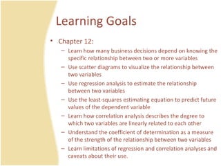
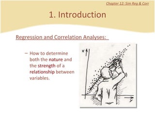
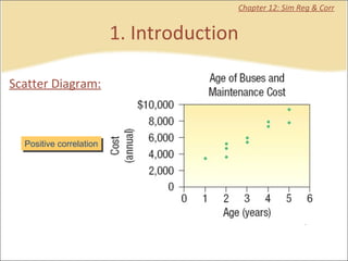
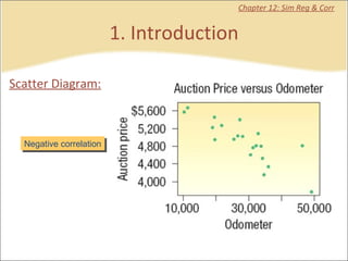
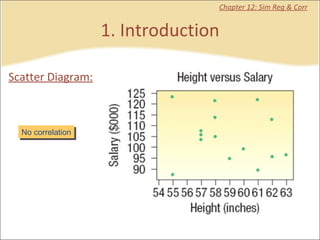
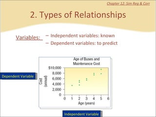
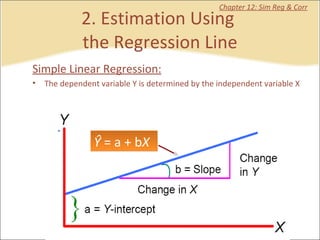
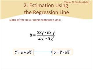
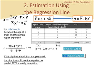
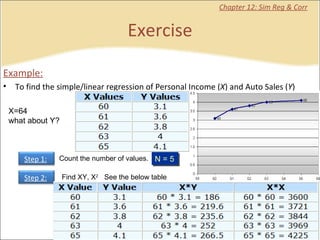
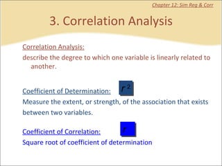
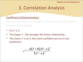
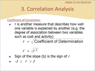
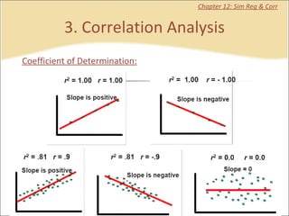
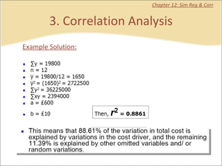
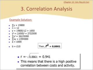
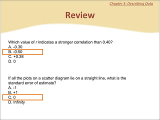
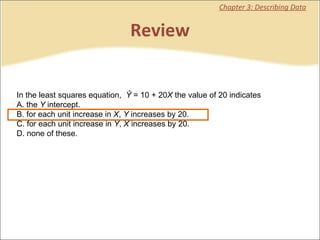
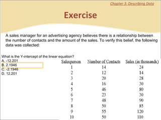
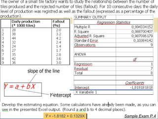
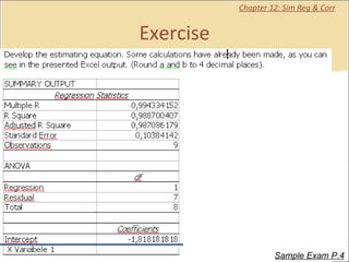
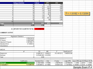
This document provides a summary of key concepts from chapters on simple regression and correlation analysis. It defines regression analysis as determining the nature and strength of relationships between variables. Scatter plots are used to visualize these relationships. The regression line estimates the relationship between an independent and dependent variable. Correlation analysis describes the degree of linear relationship between variables using the coefficient of determination and coefficient of correlation. Examples are provided to demonstrate calculating the regression equation and correlation coefficient.
This document contains summaries and examples of key concepts in regression analysis and correlation from Chapter 12, including:
- Regression analysis is used to estimate relationships between variables and predict future values of dependent variables based on independent variables.
- Correlation analysis describes the strength of the linear relationship between two variables from 0 to 1.
- The least squares method is used to fit a regression line that minimizes the squared errors between observed and predicted values.
This document summarizes key concepts from Chapter 5 of Jamri AB on correlation and simple linear regression. It introduces correlation as a measure of the strength of the linear relationship between two variables. It discusses scatter diagrams, the coefficient of correlation (r), and Pearson's product-moment correlation coefficient and Spearman's rank correlation coefficient as methods to calculate r. It also covers the coefficient of determination (r^2), linear regression analysis to predict relationships, and calculating the regression equation coefficients a and b. Examples are provided to demonstrate calculating r and the regression equation from sets of data.
The document provides information about regression analysis and calculating the coefficient of determination. It includes:
1) Instructions on how to perform a regression analysis using a calculator to find the least squares regression line, correlation coefficient, and residual plot from sample data.
2) An explanation of the coefficient of determination as a measure of how much variability in the variable y can be explained by its linear relationship with variable x.
3) A calculation example finding the coefficient of determination to be 0.83 for a dataset relating height and shoe size, meaning approximately 83% of the variation in shoe size can be explained by height.
This document discusses correlation and regression. Correlation describes the strength and direction of a linear relationship between two variables, while regression allows predicting a dependent variable from an independent variable. It provides examples of calculating the correlation coefficient r to determine the strength and direction of relationships between variables like education and self-esteem or family income and number of children. The regression equation describes the linear regression line and can be used to predict values of the dependent variable from known values of the independent variable.
The document discusses the least squares regression method for determining the line of best fit for a dataset. It explains that the least squares method finds the line that minimizes the sum of the squares of the distances between the observed responses in the dataset and the responses predicted by the linear approximation. The document provides steps to calculate the line of best fit, including calculating the slope and y-intercept. It also includes an example of applying the least squares method to find the line of best fit for a dataset relating t-shirt prices and number of t-shirts sold.
This document provides an overview of simple linear regression analysis. It discusses estimating regression coefficients using the least squares method, interpreting the regression equation, assessing model fit using measures like the standard error of the estimate and coefficient of determination, testing hypotheses about regression coefficients, and using the regression model to make predictions.
This document discusses correlation and regression analysis. It defines correlation as a mutual relationship between two or more variables, and identifies positive, negative, simple, partial and multiple correlation. Regression is defined as determining the statistical relationship between a dependent variable and one or more independent variables. Methods for calculating correlation coefficients like Pearson's r and Spearman's rank correlation coefficient are presented. Steps for determining the regression equation and calculating the slope and intercept are also outlined.
This document discusses linear regression and its use in modeling real-world problems. It defines linear regression as finding the linear function that best fits a set of data points. The document provides an example of using a graphing calculator to perform linear regression on price and weight data for emeralds. The calculator outputs an equation for the line of best fit as y = 5475x - 1042.9, providing a simple mathematical model to describe the relationship between an emerald's price and weight.
Regression analysis is used to model relationships between variables. Simple linear regression involves modeling the relationship between a single independent variable and dependent variable. The regression equation estimates the dependent variable (y) as a linear function of the independent variable (x). The parameters β0 and β1 are estimated using the method of least squares. The coefficient of determination (r2) measures how well the regression line fits the data. Additional tests like the t-test, confidence intervals, and F-test are used to test if the independent variable significantly predicts the dependent variable. While these tests can indicate a statistically significant relationship, they do not prove causation.
This document provides information about regression analysis and linear regression. It defines regression analysis as using relationships between quantitative variables to predict a dependent variable from independent variables. Linear regression finds the best fitting straight line relationship between variables. The simple linear regression equation is given as Y = a + bX, where a and b are estimated parameters calculated from sample data. An example is worked through, showing how to calculate the regression equation from data, graph the relationship, and use the equation to estimate values.
This document provides an introduction to correlation and regression analysis. It defines correlation as a measure of the association between two variables and regression as using one variable to predict another. The key aspects covered are:
- Calculating correlation using Pearson's correlation coefficient r to measure the strength and direction of association between variables.
- Performing simple linear regression to find the "line of best fit" to predict a dependent variable from an independent variable.
- Using a TI-83 calculator to graphically display scatter plots of data and calculate the regression equation and correlation coefficient.
This document provides an introduction to basic statistics and regression analysis. It defines regression as relating to or predicting one variable based on another. Regression analysis is useful for economics and business. The document outlines the objectives of understanding simple linear regression, regression coefficients, and merits and demerits of regression analysis. It describes types of regression including simple and multiple regression. Key concepts explained in more detail include regression lines, regression equations, regression coefficients, and the difference between correlation and regression. Examples are provided to demonstrate calculating regression equations using different methods.
This document discusses Spearman's rank correlation coefficient, a non-parametric measure of statistical dependence between two variables. It does not assume a normal distribution like other correlation coefficients. The Spearman coefficient is calculated by ranking the values of each variable separately and then calculating the difference between their ranks, summing the squared differences, and dividing by the number of samples. The document provides an example calculation of the Spearman coefficient between two variables and its interpretation.
- The class outline covers regression analysis, including determining the R-squared value and interpreting regression output from Excel.
- Regression models the relationship between a dependent variable (sales) and independent variables (price and other factors) using estimated coefficients.
- The R-squared value measures the explanatory power of the regression model, with higher values indicating more of the variation in the dependent variable is explained by the independent variables.
- Excel can be used to perform the regression analysis and output statistics including coefficients, F-statistics from the ANOVA table, and p-values to interpret the significance of each coefficient.
The document discusses simple linear regression and correlation. It explains how to calculate the slope and intercept of a regression line by using a scatterplot of two variables to visualize their relationship. It then shows how to compute Pearson's correlation coefficient r to quantify the strength of the linear relationship, with r closer to 1 indicating a stronger correlation. The example computes the slope, intercept, r, and tests if the correlation is statistically significant for a sample dataset about soda consumption and bathroom trips.
Ordinary least squares linear regressionElkana Rorio
Ordinary Least Squares Linear Regression is commonly used but often misunderstood and misapplied. It works by minimizing the sum of squared errors between predictions and actual values in the training data to determine coefficients for the linear regression equation. However, it is very sensitive to outliers in the data which can dramatically affect the determined coefficients and reduce prediction accuracy. Alternative regression techniques like least absolute deviations are more robust to outliers but less computationally efficient. Preprocessing data to remove or de-emphasize outliers can help address these issues with Ordinary Least Squares regression.
1) The document discusses simple linear regression using a scatter diagram and data from a study of employees' years of working experience and income.
2) It presents the scatter diagram and shows how to draw a trend line to roughly estimate dependent variable (income) values from the independent variable (years experience).
3) Equations for the least squares linear regression line are provided, including how to calculate the standard error of estimate, which is interpreted as the standard deviation around the regression line.
The document provides an overview of regression analysis techniques including linear regression and logistic regression. It defines regression as a statistical technique to model relationships between variables, with the goal of prediction or forecasting. Linear regression finds the best fitting straight line to model relationships between a continuous dependent variable and one or more independent variables. Logistic regression is used for classification problems where the dependent variable is categorical. The document explains the key differences between linear and logistic regression techniques.
This document provides an overview of ratios, proportions, and their properties. It defines a ratio as a comparison of quantities represented using ":" and explains how to obtain a ratio by dividing the first quantity by the second. It describes the terms in a ratio and properties such as ratios being pure numbers without units. Proportions are defined as the equality of two ratios, with the four terms being the extremes and means. Direct proportion is explained as two quantities increasing or decreasing proportionally together, while inverse proportion is two quantities changing proportionally in opposite directions.
Simple Linear Regression: Step-By-StepDan Wellisch
This presentation was made to our meetup group found here.: https://www.meetup.com/Chicago-Technology-For-Value-Based-Healthcare-Meetup/ on 9/26/2017. Our group is focused on technology applied to healthcare in order to create better healthcare.
This document provides an overview of regression analysis and two-way tables. It defines key concepts such as regression lines, correlation, residuals, and marginal and conditional distributions. Regression finds the linear relationship between two variables to make predictions. The least squares regression line minimizes the vertical distance between the data points and the line. Correlation and the coefficient of determination r2 measure how well the regression line fits the data. Two-way tables summarize the relationship between two categorical variables through marginal and conditional distributions.
This document discusses correlation and linear regression. It defines correlation as a measure of the linear association between two variables. The strength of the correlation is quantified from 0 (no association) to 1 (perfect association). Regression analysis predicts the value of a dependent variable based on independent variables. Simple linear regression fits a linear equation to the data of the form Y=β0 + β1X + ε, where β0 is the Y-intercept and β1 is the slope of the regression line. The coefficient of determination, R-squared, indicates how much of the variation in the dependent variable is explained by the independent variable.
This chapter introduces simple linear regression. Simple linear regression finds the linear relationship between a dependent variable (Y) and a single independent variable (X). It estimates the regression coefficients (intercept and slope) that best predict Y from X using the least squares method. The chapter provides an example of predicting house prices from square footage. It explains how to interpret the regression coefficients and make predictions. Key outputs like the coefficient of determination (r-squared), standard error, and assumptions of the regression model are also introduced. Residual analysis is discussed as a way to check if the assumptions are met.
The document provides information on correlation and linear regression. It defines correlation as the association between two variables and discusses how the correlation coefficient r measures the strength of this linear association. It then discusses:
- Computing r from sample data
- Testing the hypothesis that r = 0 using a t-test
- Computing the linear regression equation and coefficient of determination
- Using the regression equation to make predictions when there is a significant linear correlation
Two examples are then provided to demonstrate computing r from data, testing for a significant correlation, finding the regression equation, and making a prediction.
The document discusses simple linear regression. It defines key terms like regression equation, regression line, slope, intercept, residuals, and residual plot. It provides examples of using sample data to generate a regression equation and evaluating that regression model. Specifically, it shows generating a regression equation from bivariate data, checking assumptions visually through scatter plots and residual plots, and interpreting the slope as the marginal change in the response variable from a one unit change in the explanatory variable.
Regression Analysis is simplified in this presentation. Starting with simple linear to multiple regression analysis, it covers all the statistics and interpretation of various diagnostic plots. Besides, how to verify regression assumptions and some advance concepts of choosing best models makes the slides more useful SAS program codes of two examples are also included.
This document provides an overview of key concepts in regression analysis, including simple and multiple linear regression models. It outlines 10 learning objectives for the chapter, which cover topics like developing regression equations from sample data, interpreting regression outputs, assessing model fit, and addressing violations of regression assumptions. The document also includes sample regression calculations and residual plots for a case study on predicting home renovation sales from area payroll levels.
Exploring Support Vector Regression - Signals and Systems ProjectSurya Chandra
Our team competed in a Kaggle competition to predict the bike share use as a part of their capital bike share program in Washington DC using a powerful function approximation technique called support vector regression.
This document summarizes an analysis of using Support Vector Regression (SVR) to predict bike rental data from a bike sharing program in Washington D.C. It begins with an introduction to SVR and the bike rental prediction competition. It then shows that linear regression performs poorly on this non-linear problem. The document explains how SVR maps data into higher dimensions using kernel functions to allow for non-linear fits. It concludes by outlining the derivation of the SVR method using kernel functions to simplify calculations for the regression.
Please Subscribe to this Channel for more solutions and lectures
http://www.youtube.com/onlineteaching
Chapter 10: Correlation and Regression
10.2: Regression
The document compares linear regression using gradient descent and normal equations on two datasets. For the FRIED dataset, gradient descent without regularization had the best results. Adding higher degree polynomials and variable multiplications increased the model complexity but led to overfitting. For the ABALONE dataset, gradient descent with lambda=0.03 performed best. Normal equations was faster for the smaller ABALONE dataset but slower for the larger FRIED dataset due to its cubic runtime complexity. Increasing the model complexity provided better fits to the training data but risked overfitting.
This document discusses correlation and regression analysis. It begins by outlining the chapter's objectives and providing an introduction to investigating relationships between variables using statistical analysis. The document then presents examples of collecting data to study potential relationships between variables like stone dimensions, human heights and weights, and sprint and long jump performances. It introduces various statistical measures for quantifying relationships in data, including covariance, Pearson's product moment correlation coefficient, and Spearman's rank correlation coefficient. Examples are provided to demonstrate calculating and interpreting these statistics. Limitations of correlation analysis are also noted.
1. This document discusses linear regression and correlation through analyzing the relationship between two variables.
2. It introduces the concepts of scatter plots, lines of best fit, slope, and the correlation coefficient.
3. Key steps in linear regression are determining the linear equation that best models the data using least squares regression and interpreting the slope and strength of correlation.
The document provides additional information on correlation analysis. It discusses various examples of correlation between variables like sugar consumption and activity level. It explains the characteristics of a relationship such as the direction, form, and degree of correlation. Correlations can be used for prediction, validity, and reliability. The document also discusses the difference between correlation and causation. It then provides examples to test the reader's understanding of correlation through multiple choice questions. Finally, it covers topics like probable error, coefficient of correlation, coefficient of determination, Spearman's rank correlation method, and concurrent deviation method for calculating correlation.
- Regression analysis is used to study the relationship between variables and predict how the value of one variable changes with the other. It is one of the most commonly used tools for business analysis.
- Simple linear regression analyzes the relationship between one independent variable and one dependent variable. The regression equation estimates the dependent variable as a linear function of the independent variable.
- Least squares regression fits a line to the data by minimizing the sum of the squared residuals, providing estimates of the slope and y-intercept coefficients in the regression equation.
This chapter discusses regression models, including simple and multiple linear regression. It covers developing regression equations from sample data, measuring the fit of regression models, and assumptions of regression analysis. Key aspects covered include using scatter plots to examine relationships between variables, calculating the slope, intercept, coefficient of determination, and correlation coefficient, and performing hypothesis tests to determine if regression models are statistically significant. The chapter objectives are to help students understand and appropriately apply simple, multiple, and nonlinear regression techniques.
The document defines correlation and regression, and describes how to calculate them. Correlation measures the strength and direction of a linear relationship between two random variables on a scale from -1 to 1. Regression finds the linear relationship between a random variable and a fixed variable to make predictions. The document provides examples of calculating correlation using Pearson's r and determining the regression line and equation from sample data.
This document provides information about determinants of square matrices:
- It defines the determinant of a matrix as a scalar value associated with the matrix. Determinants are computed using minors and cofactors.
- Properties of determinants are described, such as how determinants change with row/column operations or identical rows/columns.
- Examples are provided to demonstrate computing determinants by expanding along rows or columns and using cofactors and minors.
- Applications of determinants include finding the area of triangles and solving systems of linear equations.
This chapter discusses building multiple regression models. It covers nonlinear variables in regression, qualitative variables and how to use them, and different model building techniques like stepwise regression, forward selection and backward elimination. The chapter aims to help students analyze and interpret nonlinear models, understand dummy variables, and learn how to build and evaluate multiple regression models and detect influential observations. It provides examples of solving regression problems and interpreting their results.
Bba 3274 qm week 6 part 1 regression modelsStephen Ong
This document provides an overview and outline of regression models and forecasting techniques. It discusses simple and multiple linear regression analysis, how to measure the fit of regression models, assumptions of regression models, and testing models for significance. The goals are to help students understand relationships between variables, predict variable values, develop regression equations from sample data, and properly apply and interpret regression analysis.
This document discusses using simple linear regression to describe relationships between variables in data. It explains that regression finds the linear equation that best describes how a dependent variable (y) changes with an independent variable (x). The equation is the line that minimizes the sum of the squared residuals (deviations from the observed data points). Examples are given of regression analyses conducted to estimate the cost of computer networks based on number of computers, estimate real estate values based on house size, and forecast housing starts based on mortgage rates.
1. The document discusses matrices and determinants. It defines different types of matrices such as rectangular, square, diagonal, scalar, row, column, identity, zero, upper triangular, and lower triangular matrices.
2. It explains how to calculate determinants of matrices. The determinant of a 1x1 matrix is the single element. The determinant of a 2x2 matrix is calculated using a formula. Determinants of higher order matrices are calculated by expanding along rows or columns.
3. It introduces concepts of minors, cofactors, and explains how the value of a determinant can be written in terms of its minors and cofactors. It also lists some properties and operations for determinants.
1. The document discusses matrices and determinants, including types of matrices like rectangular, square, diagonal, and scalar matrices.
2. It defines determinants and provides rules for computing determinants of matrices of order 2 and 3 by expanding along rows or columns.
3. Key concepts covered include minors, cofactors, properties of determinants like how row operations affect the determinant value, and examples of computing determinants.
Regression is a statistical technique used to model relationships between variables. The key steps are to identify variables, select a dependent variable to predict, examine relationships visually, and find a way to predict the dependent variable using other variables. Correlation coefficients measure the strength of relationships between 0-1. Positive relationships have variables moving in the same direction, while negative relationships have them moving in opposite directions. Non-linear regression can model curvilinear relationships using quadratic terms. Logistic regression is used for categorical dependent variables.
This document defines correlation and correlation analysis. It provides examples of how to construct scatter plots to explore relationships between two variables. Positive correlation is shown by points sloping upwards to the right on a scatter plot, while negative correlation is shown by points sloping downwards to the right. The Pearson correlation coefficient measures the strength and direction of linear relationships between variables and ranges from -1 to 1. A value close to 0 indicates a weak relationship, while values close to 1 or -1 indicate a strong positive or negative relationship, respectively. Hypothesis tests can determine if observed correlation coefficients are statistically significant. Nonparametric methods like the Spearman rank correlation can be used if the data is not interval scaled.
The document provides an overview of topics to be covered in Chapter 16 on time series and forecasting, including using trend equations to forecast future periods and develop seasonally adjusted forecasts, determining and interpreting seasonal indexes, and deseasonalizing data using a seasonal index. It also includes examples of calculating seasonal indices and adjusting sales data to remove seasonal variation. The document is a lecture outline and review for a class on international business taught by Dr. Ning Ding at Hanze University of Applied Sciences Groningen.
Here are the steps to solve this problem:
1) Code the year as t = 1 for 1999, t = 2 for 2000, etc.
2) Calculate the sums: Σt = 15, ΣY = 211.9, Σt2 = 30, ΣtY = 332.5
3) b = (ΣtY - ΣtΣY/n) / (Σt2 - Σt2/n) = 6.55
4) a = Y - bX = 29.4 - 6.55(1) = 22.85
5) Ŷ = 22.85 + 6.55t
To estimate vending sales
This document provides an overview of simple linear regression and correlation. It discusses key concepts such as dependent and independent variables, scatter diagrams, regression analysis, the least-squares estimating equation, and the coefficients of determination and correlation. Scatter diagrams are used to determine the nature and strength of relationships between variables. Regression analysis finds relationships of association but not necessarily of cause and effect. The least-squares estimating equation models the dependent variable as a function of the independent variable.
This document provides an overview of central tendency measures that will be covered in Chapter 3-A, including the mean, mode, and median for both ungrouped and grouped data. It also includes examples of calculating the mean, weighted mean, and mode. The document reviews key concepts such as the difference between parameters and statistics. Overall, the document previews and reviews important concepts related to measures of central tendency that will be covered in the upcoming chapter.
Lesson 06 chapter 9 two samples test and Chapter 11 chi square testNing Ding
This document is a PowerPoint presentation about hypothesis testing for two samples and chi-square tests. It covers topics like independent and dependent sample tests, testing differences between proportions, one-tailed and two-tailed tests. Examples are provided to demonstrate how to perform two-sample t-tests, tests of proportions, and chi-square tests using contingency tables with 2 rows and 3 rows. Step-by-step instructions and formulas are given. Key chapters from the textbook are reviewed.
This document provides an outline and overview of topics covered in a course on inductive statistics, including probability distributions, sampling distributions, estimation, and hypothesis testing. Key topics discussed include interval estimation for means and proportions, using t-distributions when sample sizes are small and variances are unknown, and the basics of hypothesis testing such as null and alternative hypotheses. Examples are provided to illustrate concepts like confidence intervals for means, proportions, and hypothesis testing.
This document contains a PowerPoint presentation on inductive statistics covering topics like probability distributions, sampling distributions, estimation, hypothesis testing for means and proportions, and two-sample hypothesis tests. It provides an overview of the chapters that will be covered, examples of hypothesis tests for means and proportions when the population standard deviation is known and unknown, and examples of independent and dependent two-sample hypothesis tests for differences in means and proportions with both large and small sample sizes. Step-by-step explanations are given for conducting hypothesis tests.
The document summarizes key concepts from chapters 6 and 7 of a statistics textbook. Chapter 6 discusses sampling and calculating standard error for infinite and finite populations. Chapter 7 introduces estimation, including interval estimates and point estimates. It provides examples of calculating standard error and confidence intervals. The document also lists SPSS tips for t-tests.
This document provides an overview and summary of topics covered in a research methods course. It discusses reviewing concepts from prior lectures, including different types of research and variables. Today's lecture will cover instrumentation, validity and reliability, and threats to internal validity. Instrumentation discusses how to collect and measure data. Validity and reliability refer to the accuracy and consistency of measurements. Threats to internal validity could interfere with determining the true effect of independent variables on dependent variables.
This document provides an overview of content covered in Statistics 2, including a review of chapter 5 on sampling distributions. It includes examples of questions from quizzes on topics like the normal distribution and binomial approximation. The document also provides tips on using SPSS for descriptive statistics, such as inputting and defining variable data, and analyzing frequencies.
This document summarizes a course on research methods and techniques. It outlines the structure and requirements of the course, including reading a textbook and attending lectures. It discusses different types of research and variables. The document covers defining research problems, formulating hypotheses, research ethics, and instrumentation. Self-check exercises are provided to help students understand key concepts.
Walmart Business+ and Spark Good for Nonprofits.pdfTechSoup
"Learn about all the ways Walmart supports nonprofit organizations.
You will hear from Liz Willett, the Head of Nonprofits, and hear about what Walmart is doing to help nonprofits, including Walmart Business and Spark Good. Walmart Business+ is a new offer for nonprofits that offers discounts and also streamlines nonprofits order and expense tracking, saving time and money.
The webinar may also give some examples on how nonprofits can best leverage Walmart Business+.
The event will cover the following::
Walmart Business + (https://business.walmart.com/plus) is a new shopping experience for nonprofits, schools, and local business customers that connects an exclusive online shopping experience to stores. Benefits include free delivery and shipping, a 'Spend Analytics” feature, special discounts, deals and tax-exempt shopping.
Special TechSoup offer for a free 180 days membership, and up to $150 in discounts on eligible orders.
Spark Good (walmart.com/sparkgood) is a charitable platform that enables nonprofits to receive donations directly from customers and associates.
Answers about how you can do more with Walmart!"
ISO/IEC 27001, ISO/IEC 42001, and GDPR: Best Practices for Implementation and...PECB
Denis is a dynamic and results-driven Chief Information Officer (CIO) with a distinguished career spanning information systems analysis and technical project management. With a proven track record of spearheading the design and delivery of cutting-edge Information Management solutions, he has consistently elevated business operations, streamlined reporting functions, and maximized process efficiency.
Certified as an ISO/IEC 27001: Information Security Management Systems (ISMS) Lead Implementer, Data Protection Officer, and Cyber Risks Analyst, Denis brings a heightened focus on data security, privacy, and cyber resilience to every endeavor.
His expertise extends across a diverse spectrum of reporting, database, and web development applications, underpinned by an exceptional grasp of data storage and virtualization technologies. His proficiency in application testing, database administration, and data cleansing ensures seamless execution of complex projects.
What sets Denis apart is his comprehensive understanding of Business and Systems Analysis technologies, honed through involvement in all phases of the Software Development Lifecycle (SDLC). From meticulous requirements gathering to precise analysis, innovative design, rigorous development, thorough testing, and successful implementation, he has consistently delivered exceptional results.
Throughout his career, he has taken on multifaceted roles, from leading technical project management teams to owning solutions that drive operational excellence. His conscientious and proactive approach is unwavering, whether he is working independently or collaboratively within a team. His ability to connect with colleagues on a personal level underscores his commitment to fostering a harmonious and productive workplace environment.
Date: May 29, 2024
Tags: Information Security, ISO/IEC 27001, ISO/IEC 42001, Artificial Intelligence, GDPR
-------------------------------------------------------------------------------
Find out more about ISO training and certification services
Training: ISO/IEC 27001 Information Security Management System - EN | PECB
ISO/IEC 42001 Artificial Intelligence Management System - EN | PECB
General Data Protection Regulation (GDPR) - Training Courses - EN | PECB
Webinars: https://pecb.com/webinars
Article: https://pecb.com/article
-------------------------------------------------------------------------------
For more information about PECB:
Website: https://pecb.com/
LinkedIn: https://www.linkedin.com/company/pecb/
Facebook: https://www.facebook.com/PECBInternational/
Slideshare: http://www.slideshare.net/PECBCERTIFICATION
Leveraging Generative AI to Drive Nonprofit InnovationTechSoup
In this webinar, participants learned how to utilize Generative AI to streamline operations and elevate member engagement. Amazon Web Service experts provided a customer specific use cases and dived into low/no-code tools that are quick and easy to deploy through Amazon Web Service (AWS.)
How to Make a Field Mandatory in Odoo 17Celine George
In Odoo, making a field required can be done through both Python code and XML views. When you set the required attribute to True in Python code, it makes the field required across all views where it's used. Conversely, when you set the required attribute in XML views, it makes the field required only in the context of that particular view.
How to Setup Warehouse & Location in Odoo 17 InventoryCeline George
In this slide, we'll explore how to set up warehouses and locations in Odoo 17 Inventory. This will help us manage our stock effectively, track inventory levels, and streamline warehouse operations.
Communicating effectively and consistently with students can help them feel at ease during their learning experience and provide the instructor with a communication trail to track the course's progress. This workshop will take you through constructing an engaging course container to facilitate effective communication.
Philippine Edukasyong Pantahanan at Pangkabuhayan (EPP) CurriculumMJDuyan
(𝐓𝐋𝐄 𝟏𝟎𝟎) (𝐋𝐞𝐬𝐬𝐨𝐧 𝟏)-𝐏𝐫𝐞𝐥𝐢𝐦𝐬
𝐃𝐢𝐬𝐜𝐮𝐬𝐬 𝐭𝐡𝐞 𝐄𝐏𝐏 𝐂𝐮𝐫𝐫𝐢𝐜𝐮𝐥𝐮𝐦 𝐢𝐧 𝐭𝐡𝐞 𝐏𝐡𝐢𝐥𝐢𝐩𝐩𝐢𝐧𝐞𝐬:
- Understand the goals and objectives of the Edukasyong Pantahanan at Pangkabuhayan (EPP) curriculum, recognizing its importance in fostering practical life skills and values among students. Students will also be able to identify the key components and subjects covered, such as agriculture, home economics, industrial arts, and information and communication technology.
𝐄𝐱𝐩𝐥𝐚𝐢𝐧 𝐭𝐡𝐞 𝐍𝐚𝐭𝐮𝐫𝐞 𝐚𝐧𝐝 𝐒𝐜𝐨𝐩𝐞 𝐨𝐟 𝐚𝐧 𝐄𝐧𝐭𝐫𝐞𝐩𝐫𝐞𝐧𝐞𝐮𝐫:
-Define entrepreneurship, distinguishing it from general business activities by emphasizing its focus on innovation, risk-taking, and value creation. Students will describe the characteristics and traits of successful entrepreneurs, including their roles and responsibilities, and discuss the broader economic and social impacts of entrepreneurial activities on both local and global scales.
4. Correction of EXCEL Exercise 5 L=(8+1)*25%=2.25 Q1=133.5 L=(8+1)*75%=6.75 Q3=274.5 Interquartile Range =274.5-133.5 =141
5. Boxplot 1 2 2 4 5 7 8 9 12 Median 1 2 2 4 7 8 9 12 Quartile Q 1 =2 Q 3 =8.5 5 Interquartile Range Decile 1st D 9th D Percentile http://cnx.org/content/m11192/latest/ How to interpret?
6. Boxplot The distribution is skewed to __________ because the mean is __________the median. the right larger than http://cnx.org/content/m11192/latest/ € 20 € 2000 Q 1 = € 250 Q 3 = € 850 Median= € 350 Mean= € 450 a b
7. 0.8 1.0 1.0 1.2 1.2 1.3 1.5 1.7 2.0 2.0 2.1 2.2 4.0 2.0 3.2 3.6 3.7 4.0 4.2 4.2 4.5 4.5 4.6 4.8 5.0 5.0 Mean > Median Mean < Median Positively skewed Negatively skewed http://qudata.com/online/statcalc/
8. This means that the data is symmetrically distributed . Zero skewness mode=median=mean
17. Chapter 12: Sim Reg & Corr Scatter Diagrams: 2. Estimation Using the Regression Line
18.
19.
20. 2. Estimation Using the Regression Line Chapter 12: Sim Reg & Corr Slope of the Best-Fitting Regression Line: Y = a + b X a = Y - b X
21. 2. Estimation Using the Regression Line Chapter 12: Sim Reg & Corr the relationship between the age of a truck and the annual repair expense? a = 6 - 0.75*3 = 3.75 Ŷ = 3.75 + 0.75 X If the city has a truck that is 4 years old, the director could use the equation to predict $675 annually in repairs. 6.75 = 3.75 + 0.75 * 4 Y = a + b X a = Y - b X X=3 Y=6
22.
23. Exercise Chapter 12: Sim Reg & Corr Find Σ X, Σ Y, Σ XY, Σ X 2 . Σ X = 311 Mean = 62.2 Σ Y = 18.6 Mean = 3.72 Σ XY = 1159.7 Σ X 2 = 19359 Step 3: Step 4: Substitute in the above slope formula given. Slope(b) = = 0.19 1159.7-5*62.2*3.72 19359-5*62.2*62.2
24. Exercise Chapter 12: Sim Reg & Corr Then substitute these values in regression equation formula Regression Equation( Ŷ ) = a + bX Ŷ = -8.098 + 0.19 X . Slope(b) = 0.19 Suppose if we want to know the approximate y value for the variable X = 64. Then we can substitute the value in the above equation. Regression Equation: Ŷ = a + bX = -8.098 + 0.19( 64 ). = -8.098 + 12.16 = 4.06 Step 5: Step 6: Now, again substitute in the above intercept formula given. Intercept(a) = Y - b X = 3.72- 0.19 * 62.2= -8.098
25. 2. Estimation Using the Regression Line Chapter 12: Sim Reg & Corr Least Squares Method: Minimize the sum of the squares of the errors to measure the goodness of fit of a line e i = residual i
26. 2. Estimation Using the Regression Line Chapter 12: Sim Reg & Corr Least Squares Method:
28. 2. Estimation Using the Regression Line Chapter 12: Sim Reg & Corr Example Solution:
29. 3. Correlation Analysis Chapter 12: Sim Reg & Corr Correlation Analysis: describe the degree to which one variable is linearly related to another. Coefficient of Determination: Measure the extent, or strength, of the association that exists between two variables. Coefficient of Correlation: Square root of coefficient of determination r 2 r
35. Review Chapter 3: Describing Data Which value of r indicates a stronger correlation than 0.40? A. -0.30 B. -0.50 C. +0.38 D. 0 If all the plots on a scatter diagram lie on a straight line, what is the standard error of estimate? A. -1 B. +1 C. 0 D. Infinity
36. Review Chapter 3: Describing Data In the least squares equation, Ŷ = 10 + 20 X the value of 20 indicates A. the Y intercept. B. for each unit increase in X , Y increases by 20. C. for each unit increase in Y , X increases by 20. D. none of these.
37. Exercise Chapter 3: Describing Data A sales manager for an advertising agency believes there is a relationship between the number of contacts and the amount of the sales. To verify this belief, the following data was collected: What is the Y-intercept of the linear equation? A. -12.201 B. 2.1946 C. -2.1946 D. 12.201
Correlation and Cause Just because two variables are correlated, does not mean that one of the variables is the cause of the other. It could be the case, but it does not necessarily follow: There is a strong positive correlation between the number of cigarettes that one smokes a day and one's chances of contracting lung cancer (measured as the number of cases of lung cancer per hundred people who smoke a given number of cigarettes). The percentage of heavy smokers who contract lung cancer is higher than the percentage of light smokers who develop the disease, and both figures are higher than the percentage of non-smokers who get lung cancer. In this case, the cigarettes are definitely causing the cancer. There is a strong negative correlation between the total number of skiing holidays that people book for any month of the year and the total amount of ice cream that supermarkets sell for that month. This means that the more skiing holidays that are booked, the less ice cream is sold. Is there a cause here? Are people spending so much money on ice cream that they can't afford skiing holidays? Is the fact that the ice cream is so cold putting people off skiing? Clearly not! The simple fact is that most people tend to book their skiing holidays in the winter, and they tend to buy ice cream in the summer. Although a correlation between two variables doesn't mean that one of them causes the other, it can suggest a way of finding out what the true cause might be. There may be some underlying variable that is causing both of them. For instance, if a survey found that there is a correlation between the time that people spend watching television and the amount of crime that people commit, it could be because unemployed people tend to sit around watching the television, and that unemployed people are more likely to commit crime. If that were the case, then unemployment would be the true cause!
More explanation: http://www.ncsu.edu/labwrite/res/gt/gt-reg-home.html