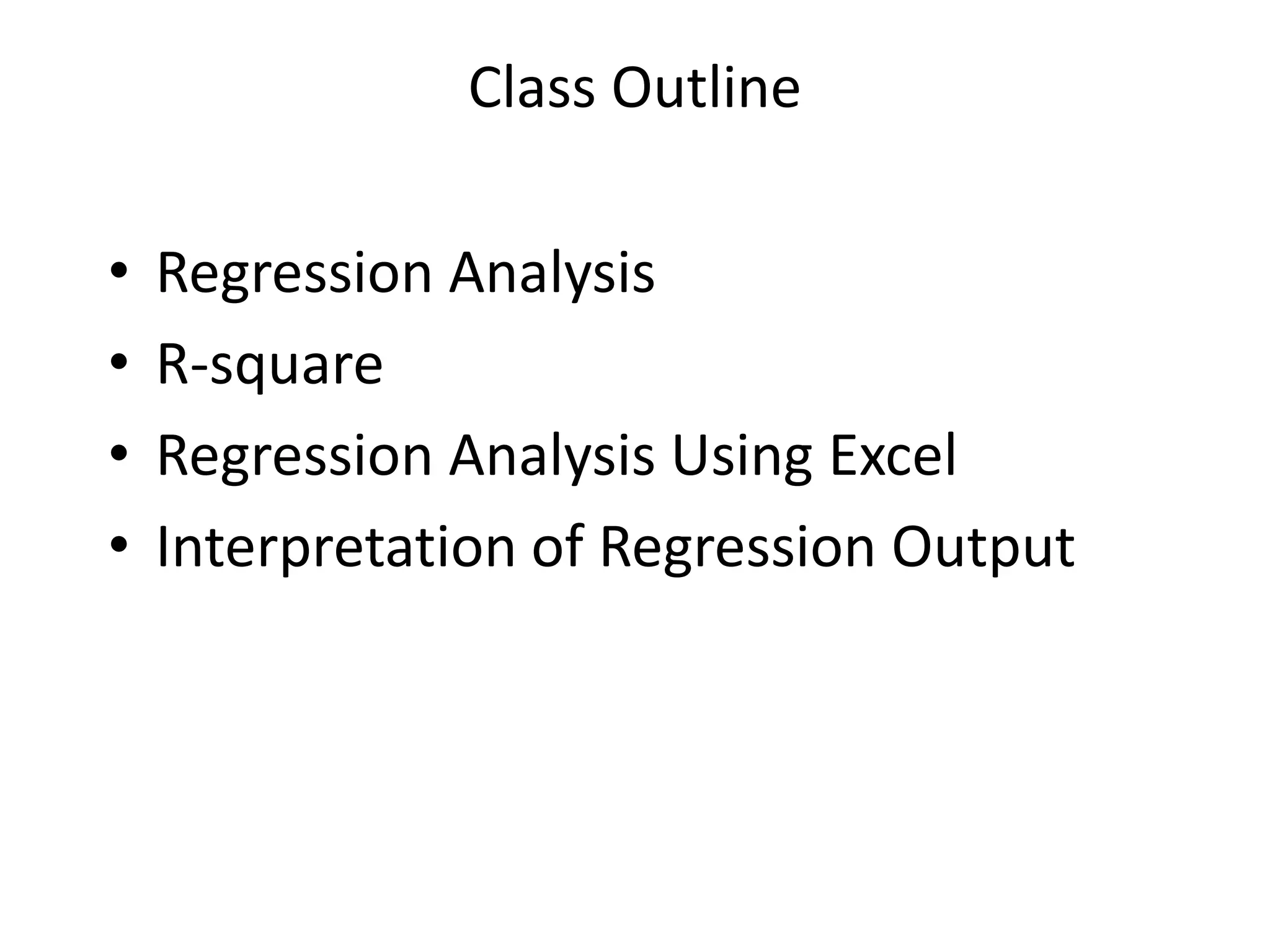
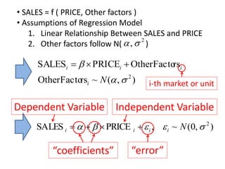
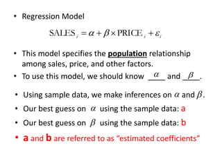
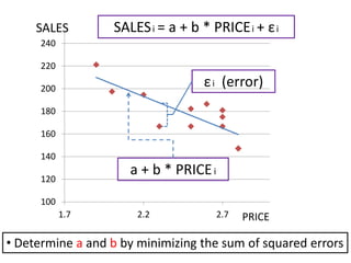
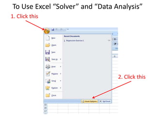
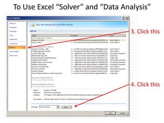
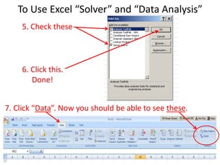
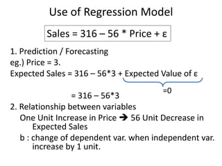
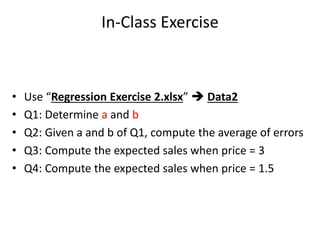
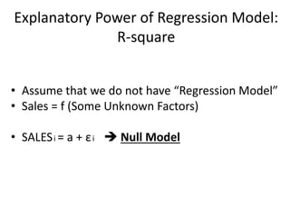
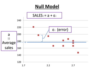
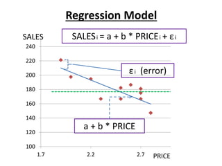
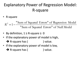
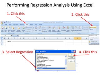
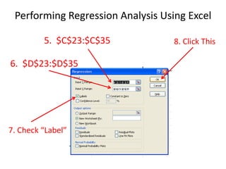
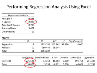
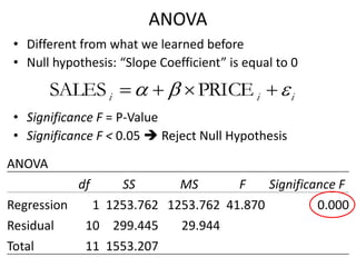
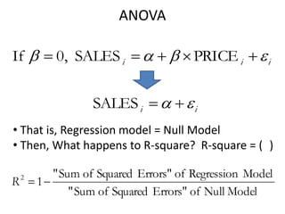
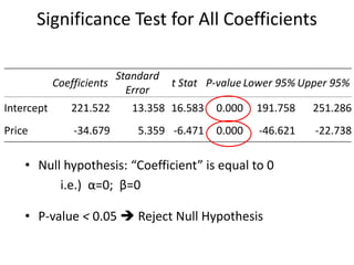
- The class outline covers regression analysis, including determining the R-squared value and interpreting regression output from Excel. - Regression models the relationship between a dependent variable (sales) and independent variables (price and other factors) using estimated coefficients. - The R-squared value measures the explanatory power of the regression model, with higher values indicating more of the variation in the dependent variable is explained by the independent variables. - Excel can be used to perform the regression analysis and output statistics including coefficients, F-statistics from the ANOVA table, and p-values to interpret the significance of each coefficient.

1. Class Outline
• Regression Analysis
• R-square
• Regression Analysis Using Excel
• Interpretation of Regression Output

2. • SALES = f ( PRICE, Other factors )
• Assumptions of Regression Model
1. Linear Relationship Between SALES and PRICE
2. Other factors follow N( )
2
,
),(~rsOtherFacto
rsOtherFactoPRICESALES
2


Ni
iii 
“error”
),0(~,PRICESALES 2
 Niiii 
“coefficients”
i-th market or unit
Independent VariableDependent Variable

3. iii   PRICESALES
• Regression Model
• This model specifies the population relationship
among sales, price, and other factors.
• To use this model, we should know ____ and ____.
• Using sample data, we make inferences on and .
• Our best guess on using the sample data: a
• Our best guess on using the sample data: b
• a and b are referred to as “estimated coefficients”
 


 

4. SALES
PRICE
100
120
140
160
180
200
220
240
1.7 2.2 2.7
a + b * PRICEi
εi (error)
• Determine a and b by minimizing the sum of squared errors
SALESi = a + b * PRICEi + εi

5. Exercise
• Determining a and b
• Use “Regression Exercise 2.xlsx”
• Use Excel “Solver” and “Data Analysis”

6. To Use Excel “Solver” and “Data Analysis”
1. Click this
2. Click this

7. To Use Excel “Solver” and “Data Analysis”
3. Click this
4. Click this

8. To Use Excel “Solver” and “Data Analysis”
5. Check these
6. Click this.
Done!
7. Click “Data”. Now you should be able to see these.

9. Use of Regression Model
1. Prediction / Forecasting
eg.) Price = 3.
Expected Sales = 316 – 56*3 + Expected Value of ε
= 316 – 56*3
2. Relationship between variables
One Unit Increase in Price  56 Unit Decrease in
Expected Sales
b : change of dependent var. when independent var.
increase by 1 unit.
Sales = 316 – 56 * Price + ε
=0

10. In-Class Exercise
• Use “Regression Exercise 2.xlsx”  Data2
• Q1: Determine a and b
• Q2: Given a and b of Q1, compute the average of errors
• Q3: Compute the expected sales when price = 3
• Q4: Compute the expected sales when price = 1.5

11. Explanatory Power of Regression:
R-square
: a measure of the _________ of
the regression model

12. Explanatory Power of Regression Model:
R-square
• Assume that we do not have “Regression Model”
• Sales = f (Some Unknown Factors)
• SALESi = a + εi  Null Model

13. a
||
Average
sales
εi (error)
SALESi = a + εi
120
140
160
180
200
220
240
1.7 2.2 2.7
Null Model

14. SALES
PRICE
100
120
140
160
180
200
220
240
1.7 2.2 2.7
a + b * PRICE
εi (error)
SALESi = a + b * PRICEi + εi
Regression Model

15. Explanatory Power of Regression Model:
R-square
• R-square
• By definition, 1 ≥ R-square ≥ 0
• If the explanatory power of model is high,
 R-square has ( ) value.
• If the explanatory power of model is low,
 R-square has ( ) value.
Null ModelofErrors"SquaredofSum"
ModelRegressionofErrors"SquaredofSum"
12
R

16. In-Class Exercise
• Use “Regression Exercise 2.xlsx”  Data2 R-
Square
• Q1: Compute R-Square

17. Performing Regression Analysis
Using Excel

18. Performing Regression Analysis Using Excel
2. Click this1. Click this
3. Select Regression 4. Click this

19. Performing Regression Analysis Using Excel
7. Check “Label”
5. $C$23:$C$35
6. $D$23:$D$35
8. Click This

20. Performing Regression Analysis Using Excel
Regression Statistics
Multiple R 0.898
R Square 0.807
Adjusted R Square 0.788
Standard Error 5.472
Observations 12
ANOVA
df SS MS F Significance F
Regression 1 1253.762 1253.762 41.870 0.000
Residual 10 299.445 29.944
Total 11 1553.207
Coefficients Standard Error t Stat P-value Lower 95% Upper 95%
Intercept 221.522 13.358 16.583 0.000 191.758 251.286
Price -34.679 5.359 -6.471 0.000 -46.621 -22.738

21. Interpretation of Regression Output

22. ANOVA
ANOVA
df SS MS F Significance F
Regression 1 1253.762 1253.762 41.870 0.000
Residual 10 299.445 29.944
Total 11 1553.207
• Different from what we learned before
• Null hypothesis: “Slope Coefficient” is equal to 0
• Significance F = P-Value
• Significance F < 0.05  Reject Null Hypothesis
iii   PRICESALES

23. ANOVA
iii   PRICESALES,0If
ii  SALES
Null ModelofErrors"SquaredofSum"
ModelRegressionofErrors"SquaredofSum"
12
R
• That is, Regression model = Null Model
• Then, What happens to R-square? R-square = ( )

24. Significance Test for All Coefficients
Coefficients
Standard
Error
t Stat P-value Lower 95% Upper 95%
Intercept 221.522 13.358 16.583 0.000 191.758 251.286
Price -34.679 5.359 -6.471 0.000 -46.621 -22.738
• Null hypothesis: “Coefficient” is equal to 0
i.e.) α=0; β=0
• P-value < 0.05  Reject Null Hypothesis