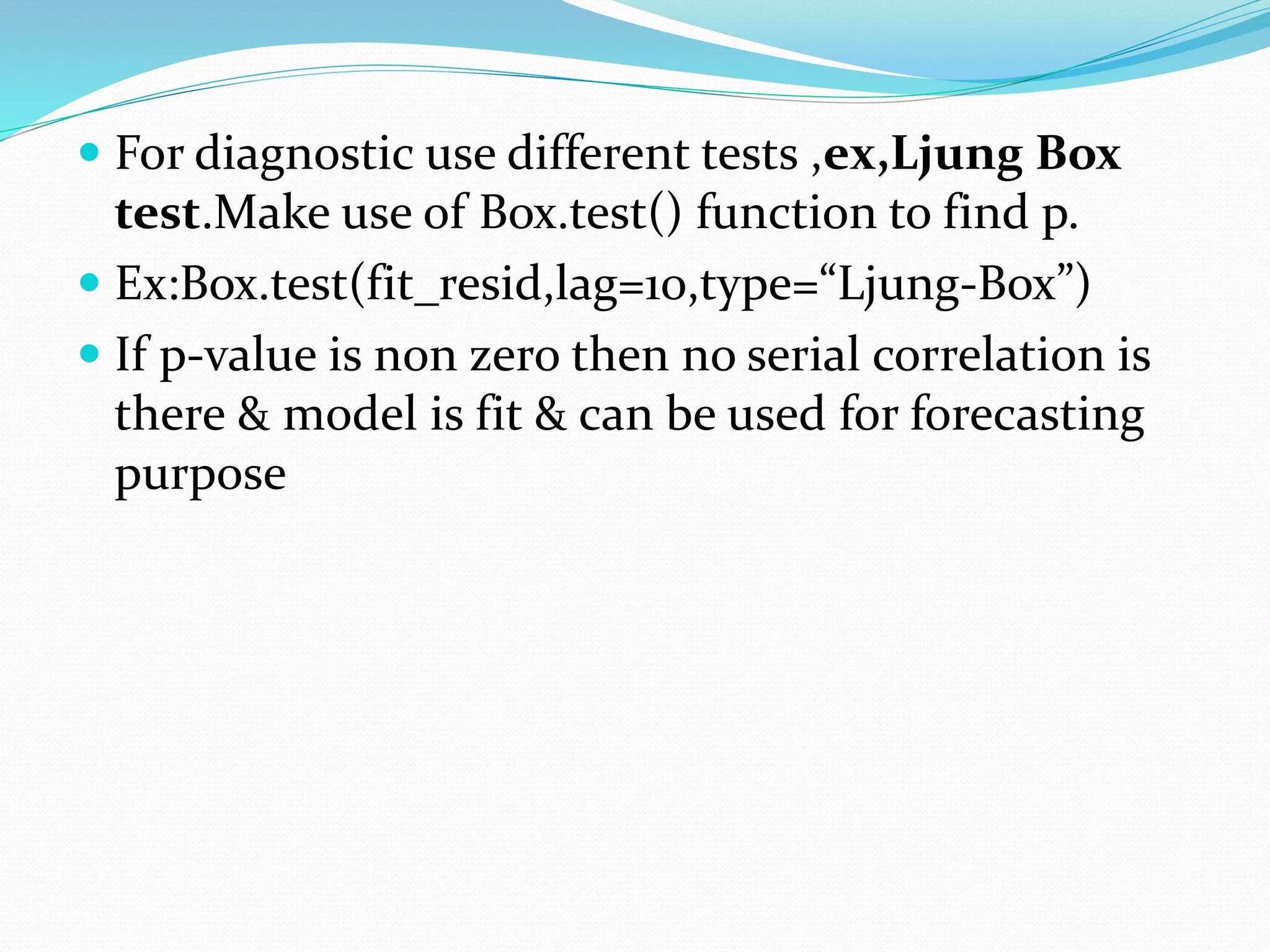
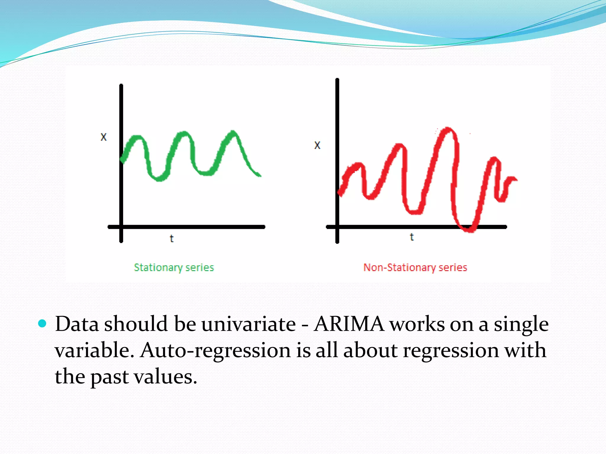
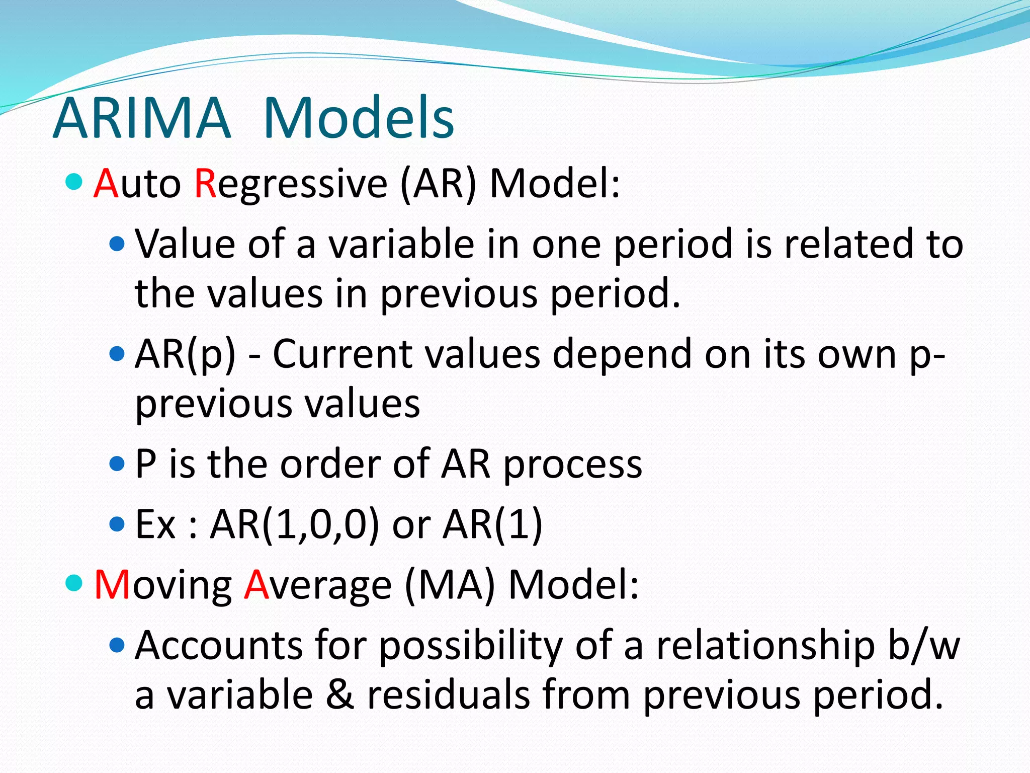
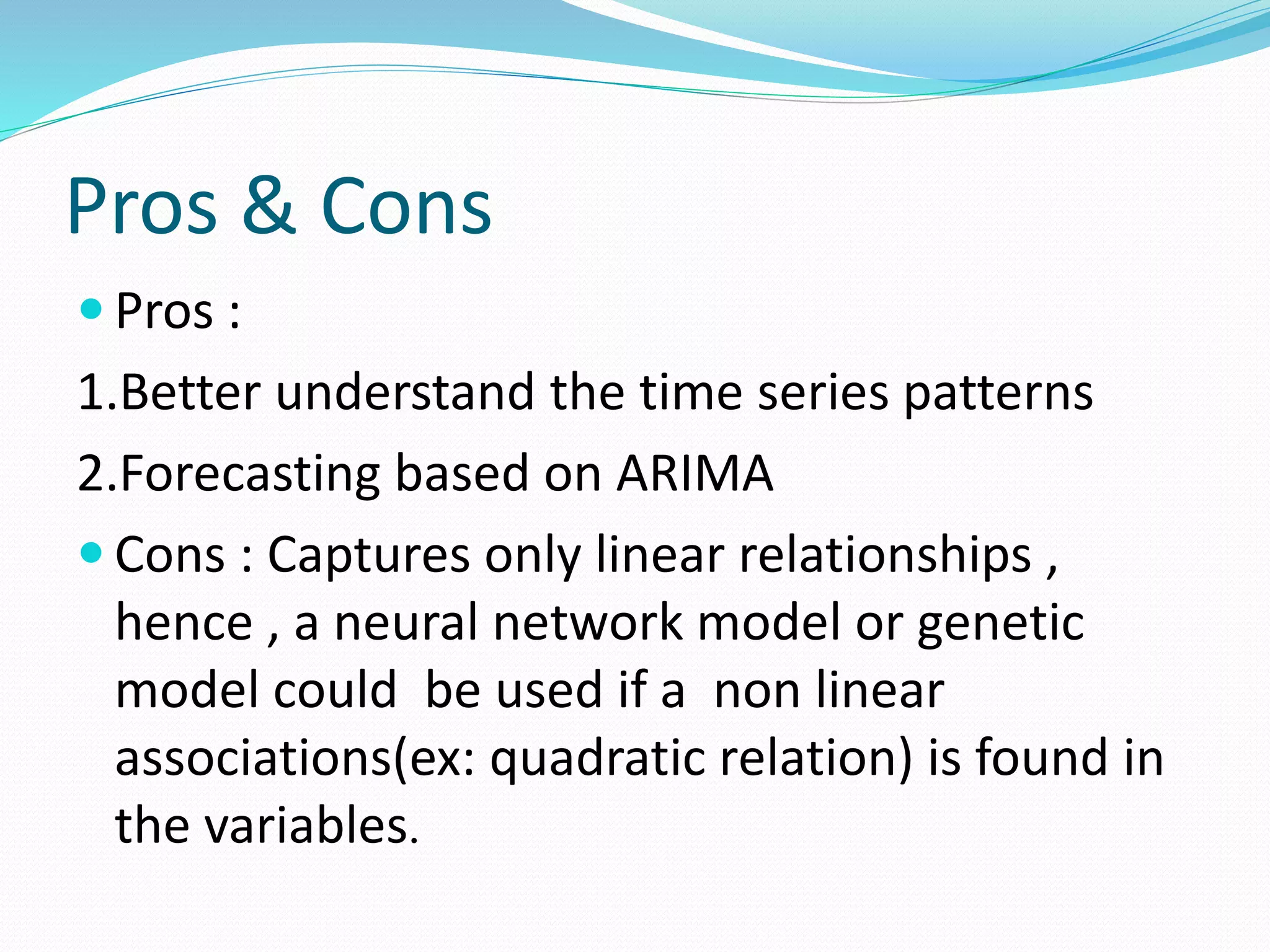
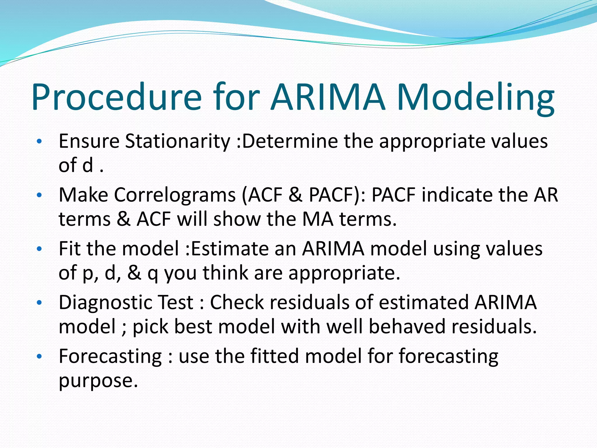
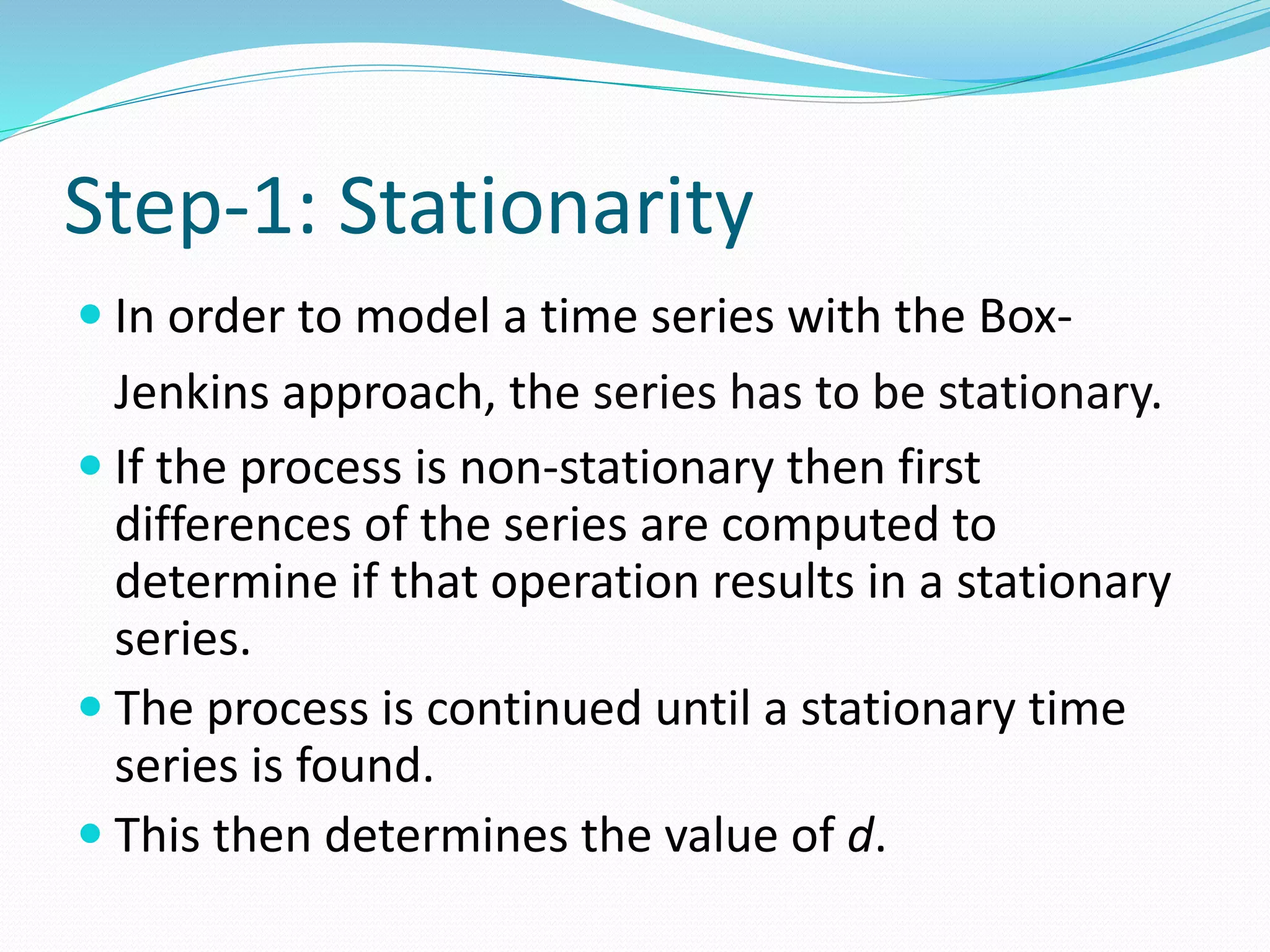
Contents
 Introduction to ARIMA
• Assumptions
 ARIMA Models
 Pros & Cons
 Procedure for ARIMA Modeling
(Box Jenkins Approach)
Introduction To ARIMA
 Acronym for Auto Regressive Integrated Moving
Average
 It is a prediction model used for time series
(time series is a collection of observations of
well-defined data items obtained through
repeated measurements over time)analysis &
forecasting.
Ex: measuring the level of unemployment each
month of the year would comprise a time series.
 A time series can also show the impact of
cyclical, seasonal and irregular events on the
data item being measured.
 Here the terms are:
Auto Regressive : lags of variables itself
Integrated :Differencing steps required to make
stationary
Moving Average :lags of previous information
shocks
 A non seasonal ARIMA model is classified as an
"ARIMA(p , d , q)" model, where:
p is the number of autoregressive terms,
d is the number of non seasonal differences
needed for stationarity, and
q is the number of lagged forecast errors in the
prediction equation.
Assumptions
 The data series used by ARIMA should be
stationary-by stationary it means that the
properties of the series doesn’t depend on the
time when it is captured. A white noise series
and series with cyclic behavior can also be
considered as stationary series.
 A non stationary series is made stationary by
differencing.
 Data should be univariate - ARIMA works on a single
variable. Auto-regression is all about regression with
the past values.
ARIMA Models
 Auto Regressive (AR) Model:
 Value of a variable in one period is related to
the values in previous period.
 AR(p) - Current values depend on its own p-
previous values
 P is the order of AR process
 Ex : AR(1,0,0) or AR(1)
 Moving Average (MA) Model:
 Accounts for possibility of a relationship b/w
a variable & residuals from previous period.
 MA(q) - The current deviation from mean
depends on q- previous deviations
 q is the order of MA process
 Only error terms are there
 Ex: MA(0,0,1) or MA(1)
 ARMA Model: both AR and MA are there,i.e,
ARMA(1,0,1) or ARMA(1,1)
 ARIMA Model : if differencing term is also
included ,i.e, ARIMA(1,1,1)=ARMA(1,1) with
first differencing
 ARIMAX: if some exogenous variables are also
included.
ARIMA+X=ARIMAX
ARIMA with environmental variable is very
important in the case when external variable
start impacting the series
Ex. Flight delay prediction depends not only
historical time series data but external variables
like weather condition (temperature , pressure,
humidity, visibility, arrival of other flights,
weighting time etc.)
Pros & Cons
 Pros :
1.Better understand the time series patterns
2.Forecasting based on ARIMA
 Cons : Captures only linear relationships ,
hence , a neural network model or genetic
model could be used if a non linear
associations(ex: quadratic relation) is found in
the variables.
Procedure for ARIMA Modeling
• Ensure Stationarity :Determine the appropriate values
of d .
• Make Correlograms (ACF & PACF): PACF indicate the AR
terms & ACF will show the MA terms.
• Fit the model :Estimate an ARIMA model using values
of p, d, & q you think are appropriate.
• Diagnostic Test : Check residuals of estimated ARIMA
model ; pick best model with well behaved residuals.
• Forecasting : use the fitted model for forecasting
purpose.
The Box-Jenkins Approach
1.Differencing the
series to achieve
stationary
2.Identify the model
3.Estimate the
parameters of the
model
Diagnostic checking.
Is the model
adequate?
No
Yes4. Use Model for forecasting
Step-1: Stationarity
 In order to model a time series with the Box-
Jenkins approach, the series has to be stationary.
 If the process is non-stationary then first
differences of the series are computed to
determine if that operation results in a stationary
series.
 The process is continued until a stationary time
series is found.
 This then determines the value of d.
Testing Stationarity
 Dickey-Fuller test
 P value has to be less than 0.05 or 5%
 If p value is greater than 0.05 or 5%, you
accept the null hypothesis, you conclude
that the time series has a unit root.
 In that case, you should first difference the
series before proceeding with analysis.
 What DF test ?
 Imagine a series where a fraction of the
current value is depending on a fraction of
previous value of the series.
 DF builds a regression line between fraction
of the current value Δyt and fraction of
previous value δyt-1
 The usual t-statistic is not valid, thus D-F
developed appropriate critical values. If P
value of DF test is <5% then the series is
stationary
Step-2:Making Correlograms
 AutoCorrelation Function (ACF):it is a
correlation coefficient. However, instead of
correlation between two different variables,
the correlation is between two values of the
same variable at times Xi and Xi+k.
 Correlation with lag-1, lag2, lag3 etc.,
 The ACF represents the degree of persistence
over respective lags of a variable.
ACF Graph
-0.50
0.000.501.00
Autocorrelationsofpresap
0 10 20 30 40
Lag
Bartlett's formula for MA(q) 95% confidence bands
 Partial Autocorrelation Function (PACF):
 The exclusive correlation coefficient
 the "partial" correlation between two variables is the
amount of correlation between them which is not
explained by their mutual correlations with a specified
set of other variables.
 For example, if we are regressing a variable Y on other
variables X1, X2, and X3, the partial correlation
between Y and X3 is the amount of correlation
between Y and X3 that is not explained by their
common correlations with X1 and X2.
 Partial correlation measures the degree of
association between two random variables, with the
effect of a set of controlling random variables removed.
PACF Graph-0.50
0.000.501.00
0 10 20 30 40
Lag
95% Confidence bands [se = 1/sqrt(n)]
Fit the Model
 Fit model based on AR & MA terms.
 Make use of auto.arima(x) function ,where x is
data series. It will do various combination of
AR & MA terms and find the best model based
on lowest AIC(Acyle Information Criteria ).
 For fitting model use arima(x,order=c(p,d,q))
function.Ex: fit=arima(x,order=c(4,0,2)).
 Order=c(p,d,q) is model received from
auto.arima(x) function.
Diagnostic Test
 First find the residuals: use residuals(model)
function.Ex: fit_resid=residuals(fit).
 Now do diagnostic on all these residuals(A
residual in forecasting is the difference
between an observed value and its forecast
based on other observations: ei=yi−y^i. For
time series forecasting, a residual is based on
one-step forecasts; that is y^t is the forecast
of yt based on observations y1,…,yt−1.).
 If residuals are IID(i.e, having no auto
correlation ) then model is fit..
 For diagnostic use different tests ,ex,Ljung Box
test.Make use of Box.test() function to find p.
 Ex:Box.test(fit_resid,lag=10,type=“Ljung-Box”)
 If p-value is non zero then no serial correlation is
there & model is fit & can be used for forecasting
purpose
Thanks

Arima model

  • 2.
    Contents  Introduction toARIMA • Assumptions  ARIMA Models  Pros & Cons  Procedure for ARIMA Modeling (Box Jenkins Approach)
  • 3.
    Introduction To ARIMA Acronym for Auto Regressive Integrated Moving Average  It is a prediction model used for time series (time series is a collection of observations of well-defined data items obtained through repeated measurements over time)analysis & forecasting. Ex: measuring the level of unemployment each month of the year would comprise a time series.
  • 4.
     A timeseries can also show the impact of cyclical, seasonal and irregular events on the data item being measured.  Here the terms are: Auto Regressive : lags of variables itself Integrated :Differencing steps required to make stationary Moving Average :lags of previous information shocks
  • 5.
     A nonseasonal ARIMA model is classified as an "ARIMA(p , d , q)" model, where: p is the number of autoregressive terms, d is the number of non seasonal differences needed for stationarity, and q is the number of lagged forecast errors in the prediction equation.
  • 6.
    Assumptions  The dataseries used by ARIMA should be stationary-by stationary it means that the properties of the series doesn’t depend on the time when it is captured. A white noise series and series with cyclic behavior can also be considered as stationary series.  A non stationary series is made stationary by differencing.
  • 7.
     Data shouldbe univariate - ARIMA works on a single variable. Auto-regression is all about regression with the past values.
  • 8.
    ARIMA Models  AutoRegressive (AR) Model:  Value of a variable in one period is related to the values in previous period.  AR(p) - Current values depend on its own p- previous values  P is the order of AR process  Ex : AR(1,0,0) or AR(1)  Moving Average (MA) Model:  Accounts for possibility of a relationship b/w a variable & residuals from previous period.
  • 9.
     MA(q) -The current deviation from mean depends on q- previous deviations  q is the order of MA process  Only error terms are there  Ex: MA(0,0,1) or MA(1)  ARMA Model: both AR and MA are there,i.e, ARMA(1,0,1) or ARMA(1,1)  ARIMA Model : if differencing term is also included ,i.e, ARIMA(1,1,1)=ARMA(1,1) with first differencing  ARIMAX: if some exogenous variables are also included.
  • 10.
    ARIMA+X=ARIMAX ARIMA with environmentalvariable is very important in the case when external variable start impacting the series Ex. Flight delay prediction depends not only historical time series data but external variables like weather condition (temperature , pressure, humidity, visibility, arrival of other flights, weighting time etc.)
  • 11.
    Pros & Cons Pros : 1.Better understand the time series patterns 2.Forecasting based on ARIMA  Cons : Captures only linear relationships , hence , a neural network model or genetic model could be used if a non linear associations(ex: quadratic relation) is found in the variables.
  • 12.
    Procedure for ARIMAModeling • Ensure Stationarity :Determine the appropriate values of d . • Make Correlograms (ACF & PACF): PACF indicate the AR terms & ACF will show the MA terms. • Fit the model :Estimate an ARIMA model using values of p, d, & q you think are appropriate. • Diagnostic Test : Check residuals of estimated ARIMA model ; pick best model with well behaved residuals. • Forecasting : use the fitted model for forecasting purpose.
  • 13.
    The Box-Jenkins Approach 1.Differencingthe series to achieve stationary 2.Identify the model 3.Estimate the parameters of the model Diagnostic checking. Is the model adequate? No Yes4. Use Model for forecasting
  • 14.
    Step-1: Stationarity  Inorder to model a time series with the Box- Jenkins approach, the series has to be stationary.  If the process is non-stationary then first differences of the series are computed to determine if that operation results in a stationary series.  The process is continued until a stationary time series is found.  This then determines the value of d.
  • 15.
    Testing Stationarity  Dickey-Fullertest  P value has to be less than 0.05 or 5%  If p value is greater than 0.05 or 5%, you accept the null hypothesis, you conclude that the time series has a unit root.  In that case, you should first difference the series before proceeding with analysis.
  • 16.
     What DFtest ?  Imagine a series where a fraction of the current value is depending on a fraction of previous value of the series.  DF builds a regression line between fraction of the current value Δyt and fraction of previous value δyt-1  The usual t-statistic is not valid, thus D-F developed appropriate critical values. If P value of DF test is <5% then the series is stationary
  • 17.
    Step-2:Making Correlograms  AutoCorrelationFunction (ACF):it is a correlation coefficient. However, instead of correlation between two different variables, the correlation is between two values of the same variable at times Xi and Xi+k.  Correlation with lag-1, lag2, lag3 etc.,  The ACF represents the degree of persistence over respective lags of a variable.
  • 18.
    ACF Graph -0.50 0.000.501.00 Autocorrelationsofpresap 0 1020 30 40 Lag Bartlett's formula for MA(q) 95% confidence bands
  • 19.
     Partial AutocorrelationFunction (PACF):  The exclusive correlation coefficient  the "partial" correlation between two variables is the amount of correlation between them which is not explained by their mutual correlations with a specified set of other variables.  For example, if we are regressing a variable Y on other variables X1, X2, and X3, the partial correlation between Y and X3 is the amount of correlation between Y and X3 that is not explained by their common correlations with X1 and X2.  Partial correlation measures the degree of association between two random variables, with the effect of a set of controlling random variables removed.
  • 20.
    PACF Graph-0.50 0.000.501.00 0 1020 30 40 Lag 95% Confidence bands [se = 1/sqrt(n)]
  • 21.
    Fit the Model Fit model based on AR & MA terms.  Make use of auto.arima(x) function ,where x is data series. It will do various combination of AR & MA terms and find the best model based on lowest AIC(Acyle Information Criteria ).  For fitting model use arima(x,order=c(p,d,q)) function.Ex: fit=arima(x,order=c(4,0,2)).  Order=c(p,d,q) is model received from auto.arima(x) function.
  • 22.
    Diagnostic Test  Firstfind the residuals: use residuals(model) function.Ex: fit_resid=residuals(fit).  Now do diagnostic on all these residuals(A residual in forecasting is the difference between an observed value and its forecast based on other observations: ei=yi−y^i. For time series forecasting, a residual is based on one-step forecasts; that is y^t is the forecast of yt based on observations y1,…,yt−1.).  If residuals are IID(i.e, having no auto correlation ) then model is fit..
  • 23.
     For diagnosticuse different tests ,ex,Ljung Box test.Make use of Box.test() function to find p.  Ex:Box.test(fit_resid,lag=10,type=“Ljung-Box”)  If p-value is non zero then no serial correlation is there & model is fit & can be used for forecasting purpose
  • 24.