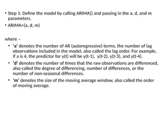
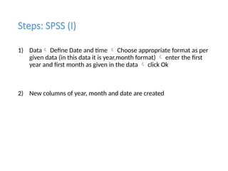
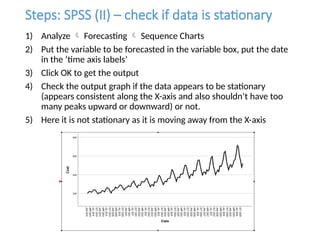
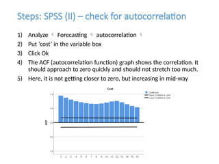
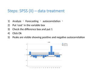
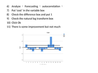
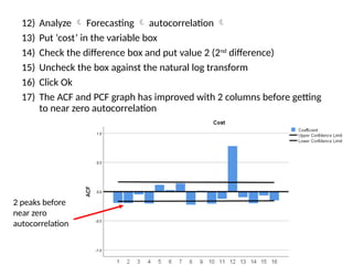
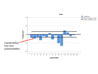
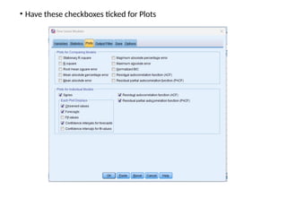
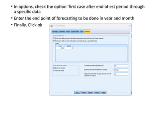
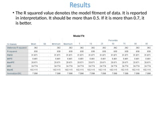
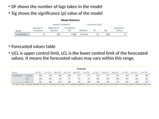
The document discusses forecasting HR costs using time series modeling, particularly the ARIMA method, essential for strategic managerial decision-making. It details the components of HR costs and outlines the steps in applying SPSS for checking data stationarity, autocorrelation, and performing the ARIMA forecast. The final results include model fit metrics, significance values, and forecasted cost ranges.

1. Forecast HR Cost Using Time Series
Modelling (ARIMA)

2. HR Cost
• HR cost is a key component of HR accounting.
• HR cost is mainly incurred from expenses related to salary, incentive,
reimbursements, insurance, and fixed and miscellaneous costs.
• This includes total cost per hired employee across an entire company, the total
compensation per employee, and the total recruitment expenditures for every
new hire across a particular time frame, expenses on job boards to draw
useful conclusions, salary of recruiters, funds required to establish an
employer brand like attending recruiting events, content writing, designing
posters and videos, social media, cost for partnerships with universities and
institutions, cost of external recruiting agencies, recruiting technology costs
like video interviewing tools, coding assessment tools.

3. Time Series Modeling
• Forecasting helps to formulate strategies in various businesses and, hence, is a basic need to
help managerial decision-making. Managers have to take decision in the face of uncertainty
without knowing what would happen.
• Forecasting can be obtained by different methods, including qualitative models and
quantitative models.
• Quantitative models include time series models and causal models.
• Causal models are used when one variable is dependent on the values of other variables.
• Time series data provide important information related to time and time series models attempt
to predict the forecast demand (future values) using the past demand values (historical data).
• Time series is a series of data points in which each data point is associated with a timestamp.
They play a major role in understanding a lot of details on specific factors with respect to time.
For example, stock price at different points of time on a given day, amount of sales in a region at
different months of the year

4. The forecasting function helps to create four types of model:
1. AR (autoregressive): A model that uses the dependent relationship between
an observation and some number of lagged observations.
2. I (integrated): The use of differencing of raw observations (e.g., subtracting
an observation from an observation at the previous time step) in order to
make the time series stationary.
3. MA (moving average): A model that uses the dependency between an
observation and a residual error from a moving average model applied to
lagged observations.
4. ARIMA (autoregressive integrated moving average): A model that has all the
above features. Each of these components are explicitly specified in the
model as a parameter. A standard notation is used for ARIMA(a, d, m) where
the parameters are substituted with integer values to quickly indicate the
specific ARIMA model being used.

5. • Step 1: Define the model by calling ARIMA() and passing in the a, d, and m
parameters.
• ARIMA=(a, d, m)
where –
• ‘a’ denotes the number of AR (autoregressive) terms, the number of lag
observations included in the model, also called the lag order. For example,
if a is 4, the predictor for y(t) will be y(t-1), y(t-2), y(t-3), and y(t-4).
• ‘d’ denotes the number of times that the raw observations are differenced,
also called the degree of differencing, number of differences, or the
number of non-seasonal differences.
• ‘m’ denotes the size of the moving average window, also called the order
of moving average.

6. Steps: SPSS (I)
1) Data Define Date and time  Choose appropriate format as per
given data (in this data it is year,month format)  enter the first
year and first month as given in the data  click Ok
2) New columns of year, month and date are created

7. Steps: SPSS (II) – check if data is stationary
1) Analyze  Forecasting  Sequence Charts
2) Put the variable to be forecasted in the variable box, put the date
in the ‘time axis labels’
3) Click OK to get the output
4) Check the output graph if the data appears to be stationary
(appears consistent along the X-axis and also shouldn’t have too
many peaks upward or downward) or not.
5) Here it is not stationary as it is moving away from the X-axis

8. Steps: SPSS (II) – check for autocorrelation
1) Analyze  Forecasting  autocorrelation 
2) Put ‘cost’ in the variable box
3) Click Ok
4) The ACF (autocorrelation function) graph shows the correlation. It
should approach to zero quickly and should not stretch too much.
5) Here, it is not getting closer to zero, but increasing in mid-way

9. Steps: SPSS (II) – data treatment
1) Analyze  Forecasting  autocorrelation 
2) Put ‘cost’ in the variable box
3) Check the difference box and put 1
4) Click Ok
5) Peaks are visible showing positive and negative autocorrelation

10. 6) Analyze  Forecasting  autocorrelation 
7) Put ‘cost’ in the variable box
8) Check the difference box and put 1
9) Check the natural log transform box
10) Click Ok
11) There is some improvement but not much

11. 12) Analyze  Forecasting  autocorrelation 
13) Put ‘cost’ in the variable box
14) Check the difference box and put value 2 (2nd
difference)
15) Uncheck the box against the natural log transform
16) Click Ok
17) The ACF and PCF graph has improved with 2 columns before getting
to near zero autocorrelation
2 peaks before
near zero
autocorrelation

12. 2 peaks before
near zero
autocorrelation

13. 18) Analyze  Forecasting  Sequence Charts
19) Put the variable to be forecasted in the variable box, put the date in
the ‘time axis labels’
20) Check the difference box and put value 2
21) Click OK to get the output
22) The graph has also become more stationary

14. Performing forecasting by ARIMA
Take the value to be
forecasted in
dependent variable
box

15. • Select ARIMA from dropdown of method
• Click on criteria
• Enter the values of ARIMA model

16. • Have these checkboxes ticked for statistics

17. • Have these checkboxes ticked for Plots

18. • In options, check the option ‘first case after end of est period through
a specific data
• Enter the end point of forecasting to be done in year and month
• Finally, Click ok

19. Results
• The R squared value denotes the model fitment of data. It is reported
in interpretation. It should be more than 0.5. If it is more than 0.7, it
is better.

20. • DF shows the number of lags taken in the model
• Sig shows the significance (p) value of the model
• Forecasted values table
• UCL is upper control limit, LCL is the lower control limit of the forecasted
values. It means the forecasted values may vary within this range.

21. • The graph shows the observed and forecasted plot of cost