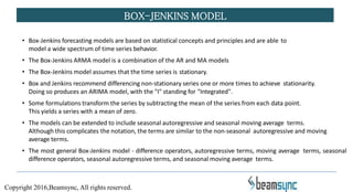
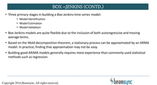
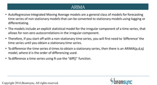
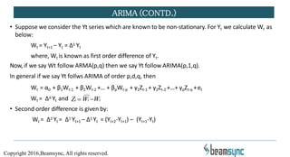
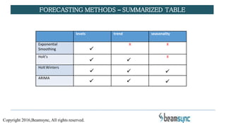
The document provides an overview of Box-Jenkins forecasting models, particularly focusing on ARIMA models for time series analysis. It describes the stages of modeling, including identification, estimation, and validation, as well as the components of AR, MA, and ARMA models. Practical applications and techniques for converting non-stationary time series to stationary ones are also discussed, emphasizing the importance of model selection based on the data's characteristics.

1. BUSINESS ANALYTICS FOUNDATION WITH R
TOOLS
Lesson 4 - Predictive Modeling Techniques
Copyright 2016,Beamsync, All rights reserved.

2. • Box-Jenkins forecasting models are based on statistical concepts and principles and are able to
model a wide spectrum of time series behavior.
• The Box-Jenkins ARMA model is a combination of the AR and MA models
• The Box-Jenkins model assumes that the time series is stationary.
• Box and Jenkins recommend differencing non-stationary series one or more times to achieve stationarity.
Doing so produces an ARIMA model, with the "I" standing for "Integrated".
• Some formulations transform the series by subtracting the mean of the series from each data point.
This yields a series with a mean of zero.
• The models can be extended to include seasonal autoregressive and seasonal moving average terms.
Although this complicates the notation, the terms are similar to the non-seasonal autoregressive and moving
average terms.
• The most general Box-Jenkins model - difference operators, autoregressive terms, moving average terms, seasonal
difference operators, seasonal autoregressive terms, and seasonal moving average terms.
BOX-JENKINS MODEL
Copyright 2016,Beamsync, All rights reserved.

3. • Three primary stages in building a Box-Jenkins time series model:
• Model Identification
• Model Estimation
• Model Validation
• Box-Jenkins models are quite flexible due to the inclusion of both autoregressive and moving
average terms.
• Based on the Wold decomposition theorem, a stationary process can be approximated by an ARMA
model. In practice, finding that approximation may not be easy.
• Building good ARIMA models generally requires more experience than commonly used statistical
methods such as regression.
BOX –JENKINS (CONTD.)
Copyright 2016,Beamsync, All rights reserved.

4. • The autoregressive (AR) process models the conditional mean of Yt as a function of past
observations of Y.
• An AR process that depends on p past observations is called an AR model of degree p, denoted by
AR(p).
• AR model can be given by:
Yt = α0 + β1Yt-1 + β2Yt-2 +… + βpYt-p +et
where, et is a series of whitenoise,
α0, β1,β2, …,βp arecoefficients.
• ACF decays down to zero as lag increases.
• PACF is non zero till k=p.
• For k>p, PACF = 0.
AUTO-REGRESSIVE (AR) MODELS
Copyright 2016,Beamsync, All rights reserved.

5. MOVING AVERAGE (MA) MODELS
• The moving average (MA) model captures serial autocorrelation in a time series Yt by expressing the
conditional mean of Yt as a function of pastinnovations.
• An MA model that depends on q past innovations is called an MA model of degree q, denoted by MA(q).
• MA model can be given by:
Yt = et + γ1et-1 + γ2et-2 +…+ γpet-p where, et
is a series of white noise ,
γ1 ,γ2 , … ,γp are coefficients.
• In reality et is not observed, so we estimate these by Zt, where Zt YtYt
• So the MA(q) model boils down to: Yt = et + γ1Zt-1 + γ2Zt-2 +…+ γpZt-q
• ACF is non-zero till k = q.
• For k > q, ACF iszero.
• PACF decays down to zero as lag increases.
Copyright 2016,Beamsync, All rights reserved.

6. • ARMA models are used in forecasting stationary models (whose mean and variance remain constant
through time, i.e., no trend effect).
• For some observed time series, a very high-order AR or MA model is needed to model the
underlying process well. In this case, a combined autoregressive moving average (ARMA) model can
sometimes be a more parsimonious choice.
• An ARMA model expresses the conditional mean of Yt as a function of both past observations, and
past innovations.
• An ARMA(p,q) model is given by:
Yt = α0 + β1Yt-1 + β2Yt-2 + … +βpYt-p + γ1Zt-1 + γ2Zt-2 +…+ γpZt-q + et
where, p denotes AR order
q denotes MA order.
ARMA
Copyright 2016,Beamsync, All rights reserved.

7. • AutoRegressive Integrated Moving Average models are a general class of models for forecasting
time series of non stationary models that can be converted to stationary models using logging or
differentiating.
• The models include an explicit statistical model for the irregular component of a time series, that
allows for non-zero autocorrelations in the irregular component.
• Therefore, if you start off with a non-stationary time series, you will first need to ‘difference’ the
time series until you obtain a stationary time series.
• Todifference the time series d times to obtain a stationary series, then there is an ARIMA(p,d,q)
model, where d is the order of differencing used.
• Todifference a time series using R use the “diff()” function.
ARIMA
Copyright 2016,Beamsync, All rights reserved.

8. ARIMA (CONTD.)
• Suppose we consider the Yt series which are known to be non-stationary. For Yt we calculate Wt as
below:
Wt = Yt+1 – Yt = Δ1 Yt
where, Wt is known as first order difference of Yt.
Now, if we say Wt follow ARMA(p,q) then we say Yt follow ARIMA(p,1,q).
In general if we say Yt follws ARIMA of order p,d,q, then
Wt = α0 + β1Wt-1 + β2Wt-2 +… + βpWt-p + γ1Zt-1 + γ2Zt-2 +…+ γpZt-q +et
Wt = Δd Yt and Zt  Wt Wt
• Second order difference is given by:
Wt = Δ2 Yt = Δ1 Yt+1 – Δ1 Yt = (Yt+2-Yt+1) – (Yt+1-Yt)
Copyright 2016,Beamsync, All rights reserved.

9. FORECASTING METHODS – SUMMARIZED TABLE
levels trend seasonality
Exponential
Smoothing
X X
Holt’s X
HoltWinters
ARIMA
Copyright 2016,Beamsync, All rights reserved.

10. Thank You
Beamsync is one of the top institutes from Bangalore, and if you are looking
for business analytics training in Bangalore, consult Beamsync. You will get
certification along with training courses. For more details click here:
http://beamsync.com/business-analytics-training-bangalore/
Copyright 2016,Beamsync, All rights reserved.