6. Approximations To Areas
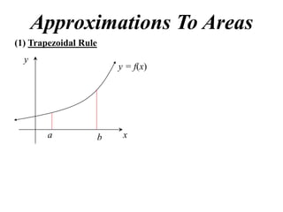
(1) Trapezoidal Rule
y
y = f(x) ba
A f a f b
2
y y = f(x)
a b x
ca bc
A f a f c f c f b
2 2
a c b x
7. Approximations To Areas
(1) Trapezoidal Rule
y
y = f(x) ba
A f a f b
2
y y = f(x)
a b x
ca bc
A f a f c f c f b
2 2
ca
f a 2 f c f b
2
a c b x
10. y
y = f(x)
ca d c
A f a f c f c f d
2 2
bd
f d f b
2
a c d b x
11. y
y = f(x)
ca d c
A f a f c f c f d
2 2
bd
f d f b
2
a c d b x c a f a 2 f c 2 f d f b
2
12. y
y = f(x)
ca d c
A f a f c f c f d
2 2
bd
f d f b
2
a c d b x c a f a 2 f c 2 f d f b
2
In general;
13. y
y = f(x)
ca d c
A f a f c f c f d
2 2
bd
f d f b
2
a c d b x c a f a 2 f c 2 f d f b
2
In general; b
Area f x dx
a
14. y
y = f(x)
ca d c
A f a f c f c f d
2 2
bd
f d f b
2
a c d b x c a f a 2 f c 2 f d f b
2
In general; b
Area f x dx
a
h
y0 2 yothers yn
2
15. y
y = f(x)
ca d c
A f a f c f c f d
2 2
bd
f d f b
2
a c d b x c a f a 2 f c 2 f d f b
2
In general; b
Area f x dx
a
h
y0 2 yothers yn
2
ba
where h
n
n number of trapeziums
16. y
y = f(x)
ca d c
A f a f c f c f d
2 2
bd
f d f b
2
a c d b x c a f a 2 f c 2 f d f b
2
In general; b
Area f x dx
a
h
y0 2 yothers yn NOTE: there is
2
ba always one more
where h function value
n
than interval
n number of trapeziums
17. e.g. Use the Trapezoida l Rule with 4 intervals to estimate the
area under the curve y 4 x , between x 0 and x 2
1
2 2
correct to 3 decimal points
18. e.g. Use the Trapezoida l Rule with 4 intervals to estimate the
area under the curve y 4 x , between x 0 and x 2
1
2 2
correct to 3 decimal points
ba
h
n
20
4
0.5
19. e.g. Use the Trapezoida l Rule with 4 intervals to estimate the
area under the curve y 4 x , between x 0 and x 2
1
2 2
correct to 3 decimal points
ba
h
n x 0 0.5 1 1.5 2
20 y 2 1.9365 1.7321 1.3229 0
4
0.5
20. e.g. Use the Trapezoida l Rule with 4 intervals to estimate the
area under the curve y 4 x , between x 0 and x 2
1
2 2
correct to 3 decimal points
ba
h
n x 0 0.5 1 1.5 2
20 y 2 1.9365 1.7321 1.3229 0
h
4 Area y0 2 yothers yn
0.5 2
21. e.g. Use the Trapezoida l Rule with 4 intervals to estimate the
area under the curve y 4 x , between x 0 and x 2
1
2 2
correct to 3 decimal points
ba 1 1
h
n x 0 0.5 1 1.5 2
20 y 2 1.9365 1.7321 1.3229 0
h
4 Area y0 2 yothers yn
0.5 2
22. e.g. Use the Trapezoida l Rule with 4 intervals to estimate the
area under the curve y 4 x , between x 0 and x 2
1
2 2
correct to 3 decimal points
ba 1 2 2 2 1
h
n x 0 0.5 1 1.5 2
20 y 2 1.9365 1.7321 1.3229 0
h
4 Area y0 2 yothers yn
0.5 2
23. e.g. Use the Trapezoida l Rule with 4 intervals to estimate the
area under the curve y 4 x , between x 0 and x 2
1
2 2
correct to 3 decimal points
ba 1 2 2 2 1
h
n x 0 0.5 1 1.5 2
20 y 2 1.9365 1.7321 1.3229 0
h
4 Area y0 2 yothers yn
0.5 2
0.5
2 21.9365 1.7321 1.3229 0
2
2.996 units 2
24. e.g. Use the Trapezoida l Rule with 4 intervals to estimate the
area under the curve y 4 x , between x 0 and x 2
1
2 2
correct to 3 decimal points
ba 1 2 2 2 1
h
n x 0 0.5 1 1.5 2
20 y 2 1.9365 1.7321 1.3229 0
h
4 Area y0 2 yothers yn
0.5 2
0.5
2 21.9365 1.7321 1.3229 0
2
2.996 units 2 exact value π
25. e.g. Use the Trapezoida l Rule with 4 intervals to estimate the
area under the curve y 4 x , between x 0 and x 2
1
2 2
correct to 3 decimal points
ba 1 2 2 2 1
h
n x 0 0.5 1 1.5 2
20 y 2 1.9365 1.7321 1.3229 0
h
4 Area y0 2 yothers yn
0.5 2
0.5
2 21.9365 1.7321 1.3229 0
2
2.996 units 2 exact value π
3.142 2.996
% error 100
3.142
4.6%
28. (2) Simpson’s Rule
b
Area f x dx
a
h
y0 4 yodd 2 yeven yn
3
29. (2) Simpson’s Rule
b
Area f x dx
a
h
y0 4 yodd 2 yeven yn
3
ba
where h
n
n number of intervals
30. (2) Simpson’s Rule
b
Area f x dx
a
h
y0 4 yodd 2 yeven yn
3
ba
where h
n
n number of intervals
e.g.
x 0 0.5 1 1.5 2
y 2 1.9365 1.7321 1.3229 0
31. (2) Simpson’s Rule
b
Area f x dx
a
h
y0 4 yodd 2 yeven yn
3
ba
where h
n
n number of intervals
e.g.
x 0 0.5 1 1.5 2
y 2 1.9365 1.7321 1.3229 0
h
Area y0 4 yodd 2 yeven yn
3
32. (2) Simpson’s Rule
b
Area f x dx
a
h
y0 4 yodd 2 yeven yn
3
ba
where h
n
n number of intervals
e.g. 1 1
x 0 0.5 1 1.5 2
y 2 1.9365 1.7321 1.3229 0
h
Area y0 4 yodd 2 yeven yn
3
33. (2) Simpson’s Rule
b
Area f x dx
a
h
y0 4 yodd 2 yeven yn
3
ba
where h
n
n number of intervals
e.g. 1 4 4 1
x 0 0.5 1 1.5 2
y 2 1.9365 1.7321 1.3229 0
h
Area y0 4 yodd 2 yeven yn
3
34. (2) Simpson’s Rule
b
Area f x dx
a
h
y0 4 yodd 2 yeven yn
3
ba
where h
n
n number of intervals
e.g. 1 4 2 4 1
x 0 0.5 1 1.5 2
y 2 1.9365 1.7321 1.3229 0
h
Area y0 4 yodd 2 yeven yn
3
35. (2) Simpson’s Rule
b
Area f x dx
a
h
y0 4 yodd 2 yeven yn
3
ba
where h
n
n number of intervals
e.g. 1 4 2 4 1
x 0 0.5 1 1.5 2
y 2 1.9365 1.7321 1.3229 0
h
Area y0 4 yodd 2 yeven yn
3
0.5
2 41.9365 1.3229 21.7321 0
3
3.084 units 2
36. (2) Simpson’s Rule
b
Area f x dx
a
h
y0 4 yodd 2 yeven yn
3
ba
where h
n
n number of intervals
e.g. 1 4 2 4 1
x 0 0.5 1 1.5 2
y 2 1.9365 1.7321 1.3229 0
h
Area y0 4 yodd 2 yeven yn
3
0.5
2 41.9365 1.3229 21.7321 0 3.142 3.084
3 % error 100
3.084 units 2 3.142
1.8%