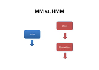
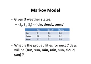
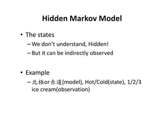
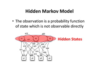
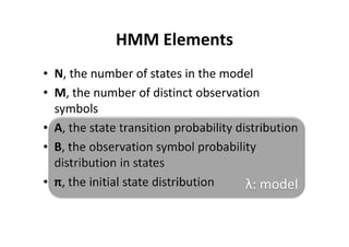
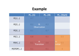
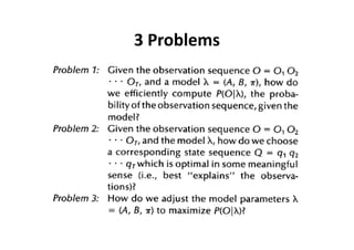
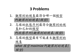
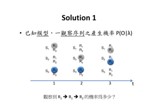
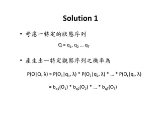
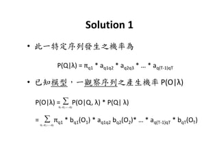
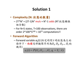
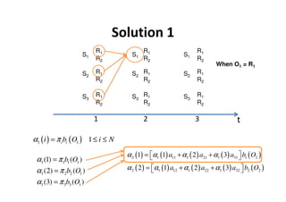
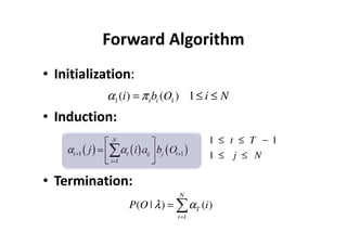
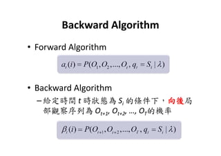
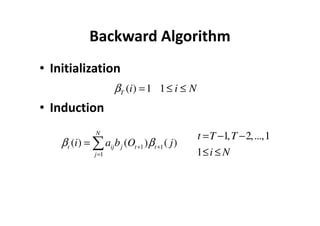
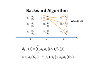
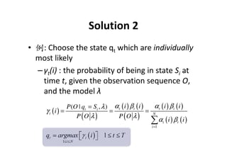
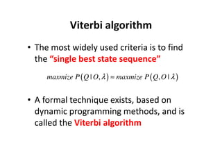
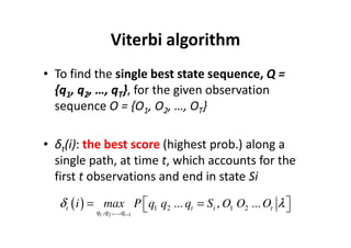
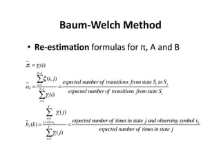
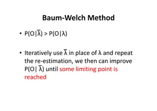
This document provides an introduction to Hidden Markov Models (HMMs). It begins by explaining the key differences between Markov Models and HMMs, noting that in HMMs the states are hidden and can only be indirectly observed through observations. It then outlines the main elements of an HMM - the number of states, observations, state transition probabilities, observation probabilities, and initial state distribution. An example HMM is provided. Finally, it briefly introduces three common problems in HMMs - determining the most likely model given observations, determining the most likely state sequence, and determining the model parameters that are most likely to have generated the observations.

1. An Introduction to HMM
Browny
2010.07.21

2. MM vs. HMM
States
States
Observations

3. Markov Model
• Given 3 weather states:
– {S1, S2, S3} = {rain, cloudy, sunny}
Rain Cloudy Sunny
Rain 0.4 0.3 0.3
Cloudy 0.2 0.6 0.2
Sunny 0.1 0.1 0.8
• What is the probabilities for next 7 days
will be {sun, sun, rain, rain, sun, cloud,
sun} ?

4. Hidden Markov Model
• The states
– We don’t understand, Hidden!
– But it can be indirectly observed
• Example
– 北極or赤道(model), Hot/Cold(state), 1/2/3
ice cream(observation)

5. Hidden Markov Model
• The observation is a probability function
of state which is not observable directly
Hidden States

6. HMM Elements
• N, the number of states in the model
• M, the number of distinct observation
symbols
• A, the state transition probability distribution
• B, the observation symbol probability
distribution in states
• π, the initial state distribution λ: model

7. Example
P(…|C) P(…|H) P(…|Start)
P(1|…) 0.7 0.1
P(2|…) 0.2 B: 0.2
Observation
P(3|…) 0.1 0.7
P(C|…) 0.8 0.1 0.5
A: π:
P(H|…) 0.1 0.8 0.5
Transition initial
P(STOP|…) 0.1 0.1 0

8. 3 Problems

9. 3 Problems
1. 觀察到的現象最符合哪一個模型
P(觀察到的現象|模型)
2. 怎樣的狀態序列最符合觀察到的現
象和已知的模型
P(狀態序列|觀察到的現象, 模型)
3. 怎樣的模型最有可能產生觀察到的
現象
what 模型 maximize P(觀察到的現象|
模型)

10. Solution 1
• 已知模型，一觀察序列之產生機率 P(O|λ)
R1 R1 R1
S1 S1 S1
R2 R2 R2
S2 R1 S2 R1 S2 R1
R2 R2 R2
S3 R1 S3 R1 S3 R1
R2 R2 R2
1 2 3 t
觀察到 R1 R1 R2 的機率為多少？

11. Solution 1
• 考慮一特定的狀態序列
Q = q1, q2 … qT
• 產生出一特定觀察序列之機率為
P(O|Q, λ) = P(O1|q1, λ) * P(O2|q2, λ) * … * P(Ot|qt, λ)
= bq1(O1) * bq2(O2) * … * bqT(OT)

12. Solution 1
• 此一特定序列發生之機率為
P(Q|λ) = πq1 * aq1q2 * aq2q3 * … * aq(T-1)qT
• 已知模型，一觀察序列之產生機率 P(O|λ)
P(O|λ) = ,q∑ q P(O|Q, λ) * P(Q| λ)
q ,...,
1 2 T
= q ,q∑ q πq1 * bq1(O1) * aq1q2 bq2(O2)* … * aq(T-1)qT * bqT(OT)
,...,
1 2 T

13. Solution 1
狀態的數量)
• Complexity (N: 狀態的數量
– 2T*NT ≈ (2T-1)NT muls + NT-1 adds (NT:狀態轉換
組合數)
– For N=5 states, T=100 observations, there are
order 2*100*5100 ≈ 1072 computations!!
• Forward Algorithm
– Forward variable αt(i) (給定時間 t 時狀態為 Si 的
條件下，向前 向前局部觀察序列為O1, O2, O3…, Ot 的
向前
機率)
at (i ) = P(O1 , O2 ,..., Ot , qt = Si | λ )

14. Solution 1
R1 R1 R1
S1 S1 S1
R2 R2 R2
When O1 = R1
S2 R1 S2 R1 S2 R1
R2 R2 R2
S3 R1 S3 R1 S3 R1
R2 R2 R2
1 2 3 t
α1 ( i ) = π i bi ( O1 ) 1 ≤ i ≤ N
α 2 (1) = α1 (1) a11 + α1 ( 2 ) a21 + α1 ( 3) a31  b1 ( O2 )
 
α1 (1) = π 1b1 (O1 )
α1 (2) = π 2b2 (O1 ) α 2 ( 2 ) = α1 (1) a12 + α1 ( 2 ) a22 + α1 ( 3) a32  b2 ( O2 )
 
α1 (3) = π 3b3 (O1 )

15. Forward Algorithm
• Initialization:
α1 (i ) = π i bi (O1 ) 1 ≤ i ≤ N
• Induction:
N  1 ≤ t ≤ T −1
αt +1 ( j ) = ∑αt ( i ) aij  bj ( Ot +1 ) 1 ≤ j ≤ N
 i=1 
• Termination:
N
P(O | λ ) = ∑ αT (i )
i =1

16. Backward Algorithm
• Forward Algorithm
at (i ) = P(O1 , O2 ,..., Ot , qt = Si | λ )
• Backward Algorithm
– 給定時間 t 時狀態為 Si 的條件下，向後 向後局
向後
部觀察序列為 Ot+1, Ot+2, …, OT的機率
βt (i ) = P(Ot +1 , Ot + 2 ,..., OT , qt = Si | λ )

17. Backward Algorithm
• Initialization
βT (i ) = 1 1 ≤ i ≤ N
• Induction
N
t = T −1, T − 2, ...,1
βt (i ) = ∑ aij b j (Ot +1 ) β t +1 ( j )
j =1 1≤ i ≤ N

18. Backward Algorithm
R1 R1 R1
S1 S1 S1
R2 R2 R2
When OT = R1
S2 R1 S2 R1 S2 R1
R2 R2 R2
S3 R1 S3 R1 S3 R1
R2 R2 R2
1 2 3 t
N
β T −1 (1) = ∑ a1 j b j ( OT ) β T ( j )
j =1
= a11b1 ( OT ) + a12 b2 ( OT ) + a13b3 ( OT )

19. Solution 2
• 怎樣的狀態序列最能解釋觀察到的現
象和已知的模型
P(狀態序列|觀察到的現象, 模型)
• 無精確解，有很多種方式解此問題，
對狀態序列的不同限制有不同的解法
對狀態序列的不同限制

20. Solution 2
• 例: Choose the state qt which are individually
most likely
– γt(i) : the probability of being in state Si at
time t, given the observation sequence O,
and the model λ
P (O | qt = Si , λ ) α t ( i ) βt ( i ) α t ( i ) βt ( i )
γ t (i ) = = = N
P (O λ ) P (O λ )
∑ α t ( i ) βt ( i )
i =1
qt = argmax γ t ( i )  1 ≤ t ≤ T
 
1≤i ≤ N

21. Viterbi algorithm
• The most widely used criteria is to find
the “single best state sequence”
maxmize P ( Q | O, λ ) ≈ maxmize P ( Q, O | λ )
• A formal technique exists, based on
dynamic programming methods, and is
called the Viterbi algorithm

22. Viterbi algorithm
• To find the single best state sequence, Q =
{q1, q2, …, qT}, for the given observation
sequence O = {O1, O2, …, OT}
• δt(i): the best score (highest prob.) along a
single path, at time t, which accounts for the
first t observations and end in state Si
δ t ( i ) = max P  q1 q2 ... qt = Si , O1 O2 ... Ot λ 
 
1 q , q ,..., q
2 t −1

23. Viterbi algorithm
• Initialization - δ1(i)
– When t = 1 the most probable path to a
state does not sensibly exist
– However we use the probability of being in
that state given t = 1 and the observable
state O1
δ1 ( i ) = π i bi ( O1 ) 1 ≤ i ≤ N
ψ (i ) = 0

24. Viterbi algorithm
• Calculate δt(i) when t > 1
– δt(i) : The most probable path to the state X
at time t
– This path to X will have to pass through one
of the states A, B or C at time (t-1)
Most probable path to A: δ t −1 ( A) a AX bX ( Ot )

25. Viterbi algorithm
• Recursion
δ t ( j ) = max δ t −1 ( i ) aij  b j ( Ot )
  2≤t ≤T
1≤ i ≤ N
ψ t ( j ) = argmax δ t −1 ( i ) aij  1≤ j ≤ N

1≤ i ≤ N

• Termination
P* = max δ T ( i ) 
 
1≤i ≤ N
q = argmax δ T ( i ) 
*
T  
1≤i ≤ N

26. Viterbi algorithm
• Path (state sequence) backtracking
qt* = ψ t +1 (qt*+1 ) t = T − 1, T − 2, ..., 1
qT −1 = ψ T (qT ) = argmax δ T −1 ( i ) aiq* 
* *
1≤i ≤ N  T 
...
...
* *
q1 = ψ 2 (q2 )

27. Solution 3
• 怎樣的模型 λ = (A, B, π) 最有可能產生
觀察到的現象
what 模型 maximize P(觀察到的現象|
模型)
• There is no known analytic solution. We
can choose λ = (A, B, π) such that P(O| λ)
is locally maximized using an iterative
procedure

28. Baum-Welch Method
• Define ξt(i, j) = P(qt=Si , qt+1=Sj|O, λ)
– The probability of being in state Si at time t,
and state Sj at time t+1
α t ( i ) aij b j ( Ot +1 ) βt +1 ( j )
ξt ( i, j ) =
P (O λ )
α t ( i ) aij b j ( Ot +1 ) βt +1 ( j )
= N N
∑∑ α ( i ) a b ( O ) β ( j )
i =1 j =1
t ij j t +1 t +1

29. Baum-Welch Method
• γt(i) : the probability of being in state Si at time
t, given the observation sequence O, and the
model λ
α t ( i ) βt ( i ) α ( i ) βt ( i )
γ t (i ) = = N t
P (O λ )
∑ α t ( i ) βt ( i )
• Relate γt(i) to ξt(i, j) i =1
α t ( i ) aij b j ( Ot +1 ) βt +1 ( j )
N ξt ( i, j ) =
γ t ( i ) = ∑ ξt ( i, j ) P (O λ )
j =1 α t ( i ) aij b j ( Ot +1 ) βt +1 ( j )
= N N
∑∑ α ( i ) a b ( O ) β ( j )
i =1 j =1
t ij j t +1 t +1

30. Baum-Welch Method
• The expected number of times that state Si is
visited
T −1
∑ γ ( i ) = Expected number of transitions from Si
t =1
t
• Similarly, the expected number of transitions
from state Si to state Sj
T −1
∑ ξ ( i, j ) = Expected number of transitions from S to S
t =1
t i j

31. Baum-Welch Method
• Re-estimation formulas for π, A and B
π i = γ1(i)
T −1
∑ξ (i, j)
t =1
t
expected number of transitions from state Si to S j
aij = T −1
=
expected number of transitions from state Si
∑γt (i)
t =1
T
∑t =1
γ t ( j)
s.t. Ot =vk expected number of times in state j and observing symbol vk
b j (k) = T
=
expected number of times in state j
∑γ ( j)
t =1
t

32. Baum-Welch Method
• P(O|λ) > P(O|λ)
• Iteratively use λ in place of λ and repeat
the re-estimation, we then can improve
P(O| λ) until some limiting point is
reached