The document discusses hidden Markov models (HMM) and their application. It begins with an introduction to HMM and covers three key algorithms: model evaluation, most probable path decoding, and model training. Successful applications of HMM include handwriting recognition, speech recognition, and gene sequence analysis. The document then provides details on Markov models as the basis for HMM, including state transition probabilities, sequence probabilities, and efficient algorithms for calculating state probabilities over time.

1. 한국정보과학회)|
한국정보과학회
KISS ILVB Tutorial(한국정보과학회 2005.04.16 |Seoul
Introduction to Hidden Markov Model
and Its Application
April 16, 2005
Dr. Sung-Jung Cho
sung-jung.cho@samsung.com
Samsung Advanced Institute of Technology (SAIT)
April 16, 2005, S.-J. Cho 1
Contents
• Introduction
• Markov Model
• Hidden Markov model (HMM)
• Three algorithms of HMM
– Model evaluation
– Most probable path decoding
– Model training
• Pattern classification by HMM
• Application of HMM to on-line handwriting recognition
with HMM toolbox for Matlab
• Summary
• References
April 16, 2005, S.-J. Cho 2

2. Sequential Data
• Data are sequentially generated according to time or
index
• Spatial information along time or index
April 16, 2005, S.-J. Cho 3
Advantage of HMM on Sequential Data
• Natural model structure: doubly stochastic process
– transition parameters model temporal variability
– output distribution model spatial variability
• Efficient and good modeling tool for
– sequences with temporal constraints
– spatial variability along the sequence
– real world complex processes
• Efficient evaluation, decoding and training algorithms
– Mathematically strong
– Computaionally efficient
• Proven technology!
– Successful stories in many applications
April 16, 2005, S.-J. Cho 4

3. Successful Application Areas of HMM
• On-line handwriting recognition
• Speech recognition
• Gesture recognition
• Language modeling
• Motion video analysis and tracking
• Protein sequence/gene sequence alignment
• Stock price prediction
• …
April 16, 2005, S.-J. Cho 5
What’s HMM?
Hidden Markov Model
Hidden + Markov Model
What is ‘hidden’? What is ‘Markov model’?
April 16, 2005, S.-J. Cho 6

4. Markov Model
• Scenario
• Graphical representation
• Definition
• Sequence probability
• State probability
April 16, 2005, S.-J. Cho 7
Markov Model: Scenario
• Classify a weather into three states
– State 1: rain or snow
– State 2: cloudy
– State 3: sunny
• By carefully examining the weather of some city for a
long time, we found following weather change pattern
Tomorrow
Rain/snow Cloudy Sunny
Tod Rain/Snow 0.4 0.3 0.3
ay
Cloudy 0.2 0.6 0.2
Sunny 0.1 0.1 0.8
Assumption: tomorrow weather depends only on today one!
April 16, 2005, S.-J. Cho 8

5. Markov Model: Graphical Representation
• Visual illustration with diagram
0.4 0.3
1: 2: 0.6
rain 0.2 cloudy
0.3 0.2
0.1 0.1
3:
sunny
0.8
- Each state corresponds to one observation
- Sum of outgoing edge weights is one
April 16, 2005, S.-J. Cho 9
Markov Model: Definition
0.4 1: 0.3 2: 0.6
• Observable states rain 0.2 cloudy
{1, 2 , L , N } 0.3 0.2
0.1
• Observed sequence 0.1
3:
q1 , q2 , L , qT sunny
0.8
• 1st order Markov assumption
P (qt = j | qt −1 = i, qt − 2 = k , L) = P ( qt = j | qt −1 = i )
L qt −1 qt −1
q1 q2 qt qt
Bayesian network representation
• Stationary
P (qt = j | qt −1 = i ) = P ( qt +l = j | qt +l −1 = i )
April 16, 2005, S.-J. Cho 10

6. Markov Model: Definition (Cont.)
0.4 0.3
• State transition matrix 1: 2: 0.6
rain 0.2 cloudy
 a11 a12 L a1 N  0.3 0.2
a a 22 L a2 N  0.1 0.1
A =  21  3:
 M M M M  sunny
 
a N1 a NN L a NN  0.8
– Where
aij = P (qt = j | qt −1 = i ), 1 ≤ i, j ≤ N
– With constraints
N
a ij ≥ 0, ∑a
j =1
ij =1
• Initial state probability
π i = P ( q 1 = i ), 1≤ i ≤ N
April 16, 2005, S.-J. Cho 11
Markov Model: Sequence Prob.
• Conditional probability
P ( A, B ) = P ( A | B ) P ( B )
• Sequence probability of Markov model
Chain rule
P ( q1 , q2 , L , qT )
= P ( q1 ) P (q2 | q1 ) L P (qT −1 | q1 , L , qT − 2 ) P (qT | q1 , L , qT −1 )
= P ( q1 ) P (q2 | q1 ) L P (qT −1 | qT − 2 ) P ( qT | qT −1 )
1st order Markov assumption
April 16, 2005, S.-J. Cho 12

7. Markov Model: Sequence Prob. (Cont.)
• Question: What is the probability that the weather for the
next 7 days will be “sun-sun-rain-rain-sun-cloudy-sun”
when today is sunny?
S1 : rain, S 2 : cloudy , S 3 : sunny
P (O | model) = P ( S 3 , S 3 , S 3 , S1 , S1 , S 3 , S 2 , S 3 | model)
= P ( S 3 ) ⋅ P ( S 3 | S 3 ) ⋅ P ( S 3 | S 3 ) ⋅ P ( S1 | S 3 )
⋅ P ( S1 | S1 ) P ( S 3 | S1 ) P ( S 2 | S 3 ) P ( S 3 | S 2 )
= π 3 ⋅ a33 ⋅ a33 ⋅ a31 ⋅ a11 ⋅ a13 ⋅ a32 ⋅ a23
= 1 ⋅ (0.8)(0.8)(0.1)(0.4)(0.3)(0.1)(0.2)
= 1.536 × 10 − 4 0.4 1:
rain
0.3 2:
cloudy
0.6
0.2
0.3 0.2
0.1 0.1
3:
sunny
April 16, 2005, S.-J. Cho 0.8 13
Markov Model: State Probability
• State probability at time t : P ( qt = i )
1 2 3 ... t
S1
S2
...
SN
• Simple but slow algorithm:
– Probability of a path that ends to state i at time t:
Qt (i ) = ( q1 , q2 , L , qt = i ) Exponential time complexity:
t
O( N t )
P (Qt (i )) = π q1 ∏ P (qk | qk −1 )
k =2
– Summation of probabilities of all the paths that ends to I at t
P ( qt = i ) = ∑ P(Q (i))
all Qt ( i )'s
t
April 16, 2005, S.-J. Cho 14

8. Markov Model: State Prob. (Cont.)
• State probability at time t : P ( qt = i )
1 2 3 ... t
S1 P ( q t −1 = 1)
S2 a 1i
...
SN
• Efficient algorithm Each node stores the sum
of probabilities of partial paths
– Recursive path probability calculation
N
P (qt = i) = ∑j =1
P ( q t −1 = j , q t = i )
N
= ∑j =1
P ( q t −1 = j ) P ( q t = i | q t −1 = j )
N
= ∑ P ( q t −1 = j ) ⋅ a ji
j =1 Time complexity: O ( N 2t )
April 16, 2005, S.-J. Cho 15
What’s HMM?
Hidden Markov Model
Hidden + Markov Model
What is ‘hidden’? What is ‘Markov model’?
April 16, 2005, S.-J. Cho 16

9. Hidden Markov Model
• Example
• Generation process
• Definition
• Model evaluation algorithm
• Path decoding algorithm
• Training algorithm
April 16, 2005, S.-J. Cho 17
Hidden Markov Model: Example
2 0.3
0.2 0.6
0.1 0.1
1 3 0.6
0.6 0.2
0.3
• N urns containing color balls
• M distinct colors
• Each urn contains different number of color balls
April 16, 2005, S.-J. Cho 18

10. HMM: Generation Process
• Sequence generating algorithm
– Step 1: Pick initial urn according to some random process
– Step 2: Randomly pick a ball from the urn and then replace it
– Step 3: Select another urn according to a random selection
process
2 0.3
– Step 4: Repeat steps 2 and 3
0.2 0.6
0.1 0.1
1 3 0.6
0.6 0.2
1 1 3 0.3
Markov process: {q(t)}
Output process: {f(x|q)}
April 16, 2005, S.-J. Cho 19
HMM: Hidden Information
• Now, what is hidden?
– We can just see the chosen balls
– We can’t see which urn is selected at a time
– So, urn selection (state transition) information is hidden
April 16, 2005, S.-J. Cho 20

11. HMM: Definition
• Notation: λ = ( Α, Β, Π )
(1) N: Number of states
(2) M: Number of symbols observable in states
V = { v1 , L , v M }
(3) A: State transition probability distribution
A = { a ij }, 1 ≤ i, j ≤ N
(4) B: Observation symbol probability distribution
B = { b i ( v k )}, 1 ≤ i ≤ N ,1 ≤ j ≤ M
(5) Π: Initial state distribution
π i = P ( q 1 = i ), 1≤ i ≤ N
April 16, 2005, S.-J. Cho 21
HMM: Dependency Structure
• 1-st order Markov assumption of transition
P ( qt | q1 , q2 , L , qt −1 ) = P ( qt | qt −1 )
• Conditional independency of observation parameters
P ( X t | qt , X 1 , L , X t −1 , q1 , L , qt −1 ) = P ( X t | qt )
q1 q2 L qt −1 qt
X1 X2 X t −1 Xt
Bayesian network representation
April 16, 2005, S.-J. Cho 22

12. HMM: Example Revisited
2 0.3
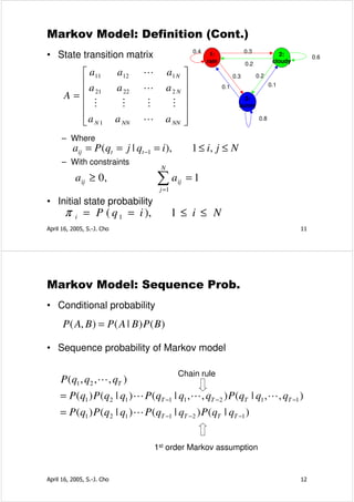
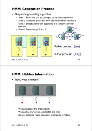
• # of states: N=3
• # of observation: M=3 0.2 0.6
V = { R, G, B } 0.1 0.1
1 3 0.6
• Initial state distribution 0.6 0.2
π = { P ( q 1 = i )} = [1 , 0 , 0 ] 0.3
• State transition probability distribution
 0 .6 0 .2 0 .2 
A = { a ij } =  0 . 1
 0 .3 0 .6 

 0 .3
 0 .1 0 .6 

• Observation symbol probability distribution
• 3 / 6 2 / 6 1 / 6 
B = { b i ( v k )} =  1 / 6
 3/6 2 / 6

1 / 6
 1/6 4 / 6

April 16, 2005, S.-J. Cho 23
0.3
HMM: Three Problems 2
0.2 0.6
0.1 0.1 0.6
• What is the probability of generating 0.6 1 0.2 3
an observation sequence? 0.3
P( )?
– Model evaluation
P ( X = x1 , x 2 , L , x T | λ ) = ? 2 0.3
0.2 0.6
0.1 0.1 0.6
• Given observation, what is the most 0.6 1 0.2 3
probable transition sequence? 0.3
– Segmentation or path analysis
*
Q = arg max Q = ( q 1 ,L , q T ) P (Q , X | λ ) 2 2 2 2
• How do we estimate or optimize
the parameters of an HMM?
2
– Training problem
P ( X | λ = ( A , B , π )) < P ( X | λ ' = ( A ' , B ' , π ' )) 1 3
April 16, 2005, S.-J. Cho 24

13. Model Evaluation
Forward algorithm
Backward algorithm
April 16, 2005, S.-J. Cho 25
Definition
• Given a model λ
• Observation sequence: X = x 1 , x 2 , L , x T
• P(X| λ) = ?
• P(X | λ) = ∑ Q
P ( X , Q | λ ) = ∑ P ( X | Q , λ ) P (Q | λ )
Q
(A path or state sequence: Q = q 1 , L , q T )
x1 x2 x3 x4 x5 x6 x7 x8 x1 x2 x3 x4 x5 x6 x7 x8
April 16, 2005, S.-J. Cho 26

14. Solution
• Easy but slow solution: exhaustive enumeration
P(X | λ) = ∑ Q
P ( X , Q | λ ) = ∑ P ( X | Q , λ ) P (Q | λ )
Q
= ∑b
Q
q1 ( x 1 ) b q 2 ( x 2 ) L b q T ( x T ) π q 1 a q 1 q 2 a q 2 q 3 L a q T −1 q T
– Exhaustive enumeration = combinational explosion!
O(N T )
• Smart solution exists?
– Yes!
– Dynamic Programming technique
– Lattice structure based computation
– Highly efficient -- linear in frame length
April 16, 2005, S.-J. Cho 27
Forward Algorithm
• Key idea
– Span a lattice of N states and T times
– Keep the sum of probabilities of all the paths coming to each
state i at time t
x1 x2 x3 x4 xt xT
Sj
• Forward probability
α t ( j ) = P( x1 x2 ...xt , qt = S j | λ )
= ∑ P( x1 x2 ...xt , Qt = q1...qt | λ )
Qt
N
= ∑ α t −1 (i )aij b j ( xt )
i =1
April 16, 2005, S.-J. Cho 28

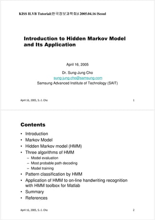
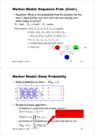
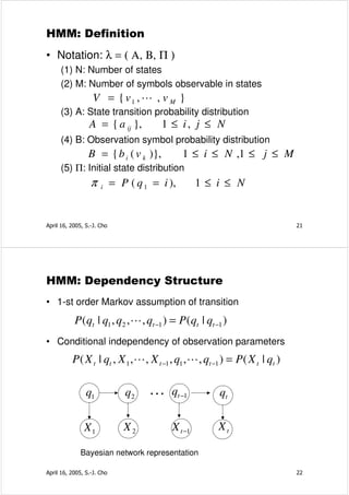
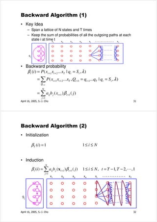
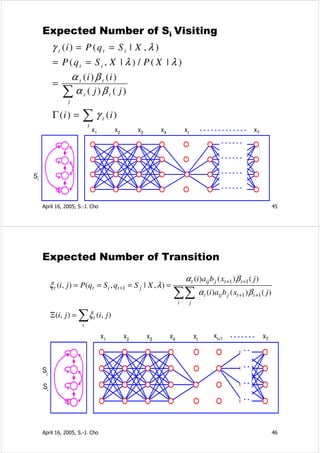
15. Forward Algorithm
• Initialization
α1 (i ) = π i bi (x1 ) 1≤ i ≤ N
• Induction
N
α t ( j ) = ∑ α t −1 (i)aij b j (x t ) 1 ≤ j ≤ N , t = 2, 3, L, T
i =1
• Termination
N
P ( X | λ ) = ∑ α T (i )
i =1 x1 x2 x3 x4 xt xT
Sj
April 16, 2005, S.-J. Cho 29
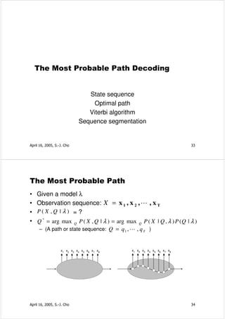
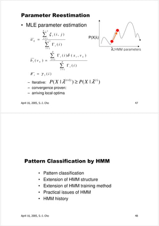
Numerical Example: P(RRGB|λ) [신봉기 03]
π =[1 0 0]T
R R G B
.5 R .6
G .2 1×.6 .5×.6 .5×.2 .5×.2
.6 .18 .018 .0018
B .2
.4 .4×.2 .4×.5 .4×.3
.6 .1 .2
0×.2 .6×.2 .6×.5 .6×.3
.5 .0 .048 .0504 .01123
.3 .1×.0 .1×.3 .1×.7
.4 .4×.0 .4×.3 .4×.7
.0 0×.0
.3 .0 .0 .01116 .01537
.7
April 16, 2005, S.-J. Cho 30

16. Backward Algorithm (1)
• Key Idea
– Span a lattice of N states and T times
– Keep the sum of probabilities of all the outgoing paths at each
state i at time t
x x x x x x
1 2 3 4 t T
Sj
• Backward probability
β t (i ) = P( xt +1 xt + 2 ...xT | qt = Si , λ )
= ∑ P( xt +1 xt + 2 ...xT , Qt +1 = qt +1...qT | qt = Si , λ )
Qt +1
N
= ∑ aij b j ( xt +1 ) β t +1 ( j )
j =1
April 16, 2005, S.-J. Cho 31
Backward Algorithm (2)
• Initialization
β T (i ) = 1 1≤ i ≤ N
• Induction
N
β t (i ) = ∑ aij b j (x t +1 ) β t +1 ( j ) 1 ≤ i ≤ N , t = T − 1, T − 2, L, 1
j =1
x1 x2 x3 x4 xt xT
Sj
April 16, 2005, S.-J. Cho 32

17. The Most Probable Path Decoding
State sequence
Optimal path
Viterbi algorithm
Sequence segmentation
April 16, 2005, S.-J. Cho 33
The Most Probable Path
• Given a model λ
• Observation sequence: X = x 1 , x 2 , L , x T
• P(X ,Q | λ) = ?
• Q * = arg max Q P ( X , Q | λ ) = arg max Q P ( X | Q , λ ) P ( Q | λ )
– (A path or state sequence: Q = q 1 , L , q T )
x1 x2 x3 x4 x5 x6 x7 x8 x1 x2 x3 x4 x5 x6 x7 x8
April 16, 2005, S.-J. Cho 34

18. Viterbi Algorithm
• Purpose
– An analysis for internal processing result
– The best, the most likely state sequence
– Internal segmentation
• Viterbi Algorithm
– Alignment of observation and state transition
– Dynamic programming technique
April 16, 2005, S.-J. Cho 35
Viterbi Path Idea
• Key idea
– Span a lattice of N states and T times
– Keep the probability and the previous node of the most probable
path coming to each state i at time t
• Recursive path selection
– Path probability: δ t +1 ( j ) = max δ t (i ) aij b j ( x t +1 )
1≤ i ≤ N
– Path node: ψ t +1 ( j ) = arg max δ t (i)aij
1≤ i ≤ N
δ t (1) a1 j b j ( x t + 1 )
t t+1
δ t ( i ) a ij b j ( x t + 1 )
Sj
April 16, 2005, S.-J. Cho 36

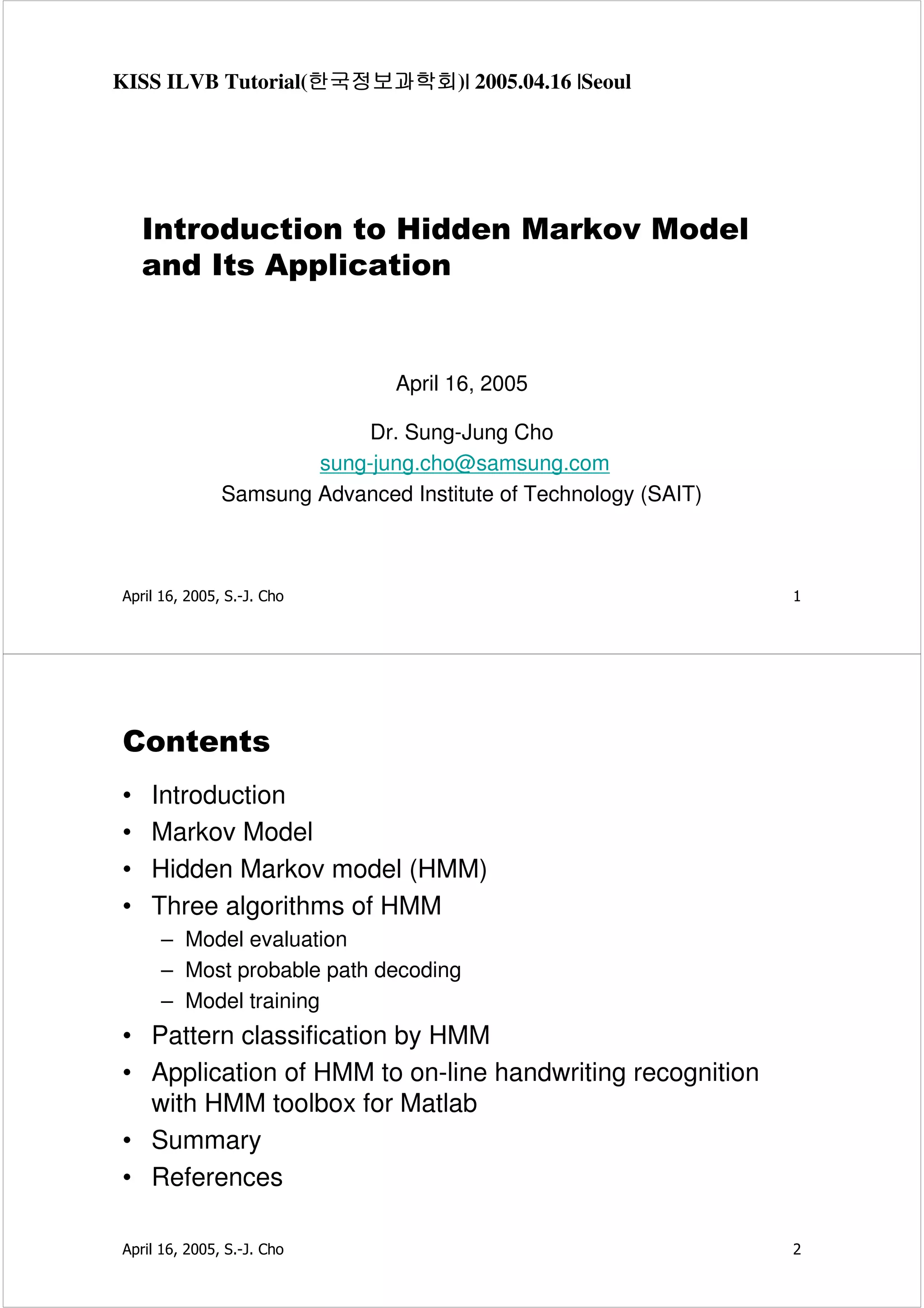
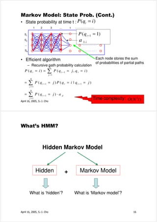
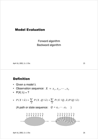
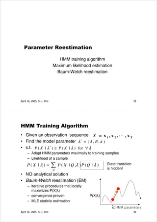
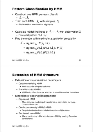
19. Viterbi Algorithm
• Introduction: δ 1 (i ) = π i bi (x1 )
ψ 1 (i ) = 0
• Recursion:
δ t +1 ( j ) = max δ t (i )aij b j (x t +1 )
1≤ i ≤ N
ψ t +1 ( j ) = arg max δ t (i)aij
1≤ i ≤ N
• Termination: P ∗ = max δ T (i )
1≤i ≤ N
∗
qT = arg max δ T (i )
1≤i ≤ N
• Path backtracking: q = ψ t +1 (qt∗+1 ), t = T − 1,K ,1
∗
t
1
states 2
3
April 16, 2005, S.-J. Cho 37
Numerical Example: P(RRGB,Q*|λ) [신봉기 03]
π =[1 0 0]T
R R G B
.5 R .6
G .2 1×.6 .5×.6 .5×.2 .5×.2
.6 .18 .018 .0018
B .2
.4 .4×.2 .4×.5 .4×.3
.6 .1 .2
0×.2 .6×.2 .6×.5 .6×.3
.5 .0 .048 .036 .00648
.3 .1×.0 .1×.3 .1×.7
.4 .4×.0 .4×.3 .4×.7
.0 0×.0
.3 .0 .0 .00576 .01008
.7
April 16, 2005, S.-J. Cho 38

20. Parameter Reestimation
HMM training algorithm
Maximum likelihood estimation
Baum-Welch reestimation
April 16, 2005, S.-J. Cho 39
HMM Training Algorithm
• Given an observation sequence X = x 1 , x 2 , L , x T
• Find the model parameter λ * = ( A , B , π )
• s.t. P ( X | λ * ) ≥ P ( X | λ ) for ∀ λ
– Adapt HMM parameters maximally to training samples
– Likelihood of a sample
P(X | λ) = ∑
Q
P ( X | Q ,λ ) P ( Q | λ ) State transition
is hidden!
• NO analytical solution
• Baum-Welch reestimation (EM)
– iterative procedures that locally
maximizes P(X|λ)
– convergence proven P(X|λ)
– MLE statistic estimation
λ:HMM parameters
April 16, 2005, S.-J. Cho 40

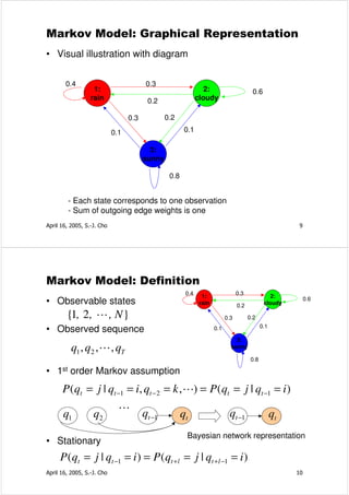
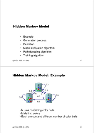
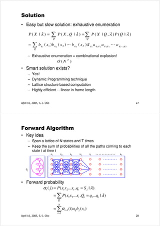
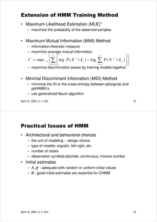
21. Maximum Likelihood Estimation
• MLE “selects those parameters that maximizes the
probability function of the observed sample.”
• [Definition] Maximum Likelihood Estimate
– Θ: a set of distribution parameters
– Given X, Θ* is maximum likelihood estimate of Θ if
– f(X|Θ*) = maxΘ f(X|Θ)
April 16, 2005, S.-J. Cho 41
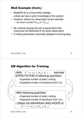
MLE Example
• Scenario
– Known: 3 balls inside urn
– (some red; some white)
– Unknown: R = # red balls
– Observation: (two reds)
• Two models  2  1  3 1
–P ( |R=2) =  2   0 
    =
2 3
    
3 3
–P ( |R=3) =  
    =1
2
2  
• Which model?
– L (λ R = 3 ) > L (λ R = 2 )
– Model(R=3) is our choice
April 16, 2005, S.-J. Cho 42

22. MLE Example (Cont.)
• Model(R=3) is a more likely strategy,
unless we have a priori knowledge of the system.
• However, without an observation of two red balls
– No reason to prefer P(λR=3) to P(λR=2)
• ML method chooses the set of parameters that
maximizes the likelihood of the given observation.
• It makes parameters maximally adapted to training data.
April 16, 2005, S.-J. Cho 43
EM Algorithm for Training
•With λ ( t ) =< { a ij }, { b ik }, π i > , estimate
EXPECTATION of following quantities:
–Expected number of state i visiting
–Expected number of transitions from i to j
•With following quantities:
–Expected number of state i visiting
–Expected number of transitions from i to j
• Obtain the MAXIMUM LIKELIHOOD of
λ ( t + 1 ) =< { a ' ij }, { b ' ik }, π i >
April 16, 2005, S.-J. Cho 44

23. Expected Number of Si Visiting
γ t (i ) = P ( q t = S i | X , λ )
= P (qt = S i , X | λ ) / P ( X | λ )
α t (i ) β t (i )
=
∑ α t ( j)β t ( j)
j
Γ (i ) = ∑γ t
t (i )
x1 x2 x3 x4 xt xT
Si
April 16, 2005, S.-J. Cho 45
Expected Number of Transition
α t (i )aij b j ( xt +1 ) β t +1 ( j )
ξ t (i, j ) = P(qt = S i , qt +1 = S j | X , λ ) =
∑∑ α (i)a b ( x
i j
i ij j t +1 ) β t +1 ( j)
Ξ (i, j ) = ∑ξ (i, j)
t
t
x1 x2 x3 x4 xt xt+1 xT
Sj
Si
April 16, 2005, S.-J. Cho 46

24. Parameter Reestimation
• MLE parameter estimation
T −1
∑
t =1
ξ t (i, j )
P(X|λ)
a ij = T −1
∑ Γt (i)
t =1
T
λ:HMM parameters
∑
t =1
Γ t ( i )δ ( x t , v k )
bi (v k ) = T
∑
t =1
Γt (i)
π i = γ 1 (i)
( t +1)
– Iterative: P ( X | λ ) ≥ P ( X | λ( t ) )
– convergence proven:
– arriving local optima
April 16, 2005, S.-J. Cho 47
Pattern Classification by HMM
• Pattern classification
• Extension of HMM structure
• Extension of HMM training method
• Practical issues of HMM
• HMM history
April 16, 2005, S.-J. Cho 48

25. Pattern Classification by HMM
• Construct one HMM per each class k
– λ1 ,L , λN
• Train each HMM λk with samples Dk
– Baum-Welch reestimation algorithm
• Calculate model likelihood of λ1 , L , λN with observation X
– Forward algorithm: P ( X | λk )
• Find the model with maximum a posteriori probability
λ* = argmax λ k P(λk | X )
= argmax λ k P(λk ) P ( X | λk ) / P( X )
= argmax λ k P(λk ) P ( X | λk )
April 16, 2005, S.-J. Cho 49
Extension of HMM Structure
• Extension of state transition parameters
– Duration modeling HMM
• More accurate temporal behavior
– Transition-output HMM
• HMM output functions are attached to transitions rather than states
• Extension of observation parameter
– Segmental HMM
• More accurate modeling of trajectories at each state, but more
computational cost
– Continuous density HMM (CHMM)
• Output distribution is modeled with mixture of Gaussian
– Semi-continuous HMM
• Mix of continuous HMM and discrete HMM by sharing Gaussian
components
April 16, 2005, S.-J. Cho 50

26. Extension of HMM Training Method
• Maximum Likelihood Estimation (MLE)*
– maximize the probability of the observed samples
• Maximum Mutual Information (MMI) Method
– information-theoretic measure
– maximize average mutual information:
 V  V

I = max λ  ∑  log P ( X
* v
| λ v ) − log ∑ P(X w
| λw ) 
 ν =1  w =1 
– maximize discrimination power by training models together
• Minimal Discriminant Information (MDI) Method
– minimize the DI or the cross entropy between pd(signal) and
pd(HMM)’s
– use generalized Baum algorithm
April 16, 2005, S.-J. Cho 51
Practical Issues of HMM
• Architectural and behavioral choices
– the unit of modeling -- design choice
– type of models: ergodic, left-right, etc.
– number of states
– observation symbols;discrete, continuous; mixture number
• Initial estimates
– A, π : adequate with random or uniform initial values
– B : good initial estimates are essential for CHMM
April 16, 2005, S.-J. Cho 52

27. Practical Issues of HMM (Cont.)
• Scaling
t −1 t
α t (i ) = ∏
s =1
a s , s +1 ∏b (x )
s =1
s s
– heads exponentially to zero: --> scale by 1 / Si=1,…,N at(i)
• Multiple observation sequences
– accumulate the expected freq. with weight P(X(k)|l)
• Insufficient training data
– deleted interpolation with desired model & small model
– output prob. smoothing (by local perturbation of symbols)
– output probability tying between different states
April 16, 2005, S.-J. Cho 53
HMM History [Roweis]
• Markov(’13) and Shannon (’48, ’51) studied Markov
chains
• Baum et. Al (BP’66, BE’67 …) developed many theories
of “probabilistic functions of Markov chains”
• Viterbi (’67) developed an efficient optimal state search
algorithm
• Application to speech recognition started
– Baker(’75) at CMU
– Jelinek’s group (’75) at IBM
• Dempster, Laird & Rubin ('77) recognized a general form
of the Baum-Welch algorithm
April 16, 2005, S.-J. Cho 54

28. Application of HMM to on-line
handwriting recognition with HMM SW
• SW tools for HMM
• Introduction to on-line handwriting
recognition
• Data preparation
• Training & testing
April 16, 2005, S.-J. Cho 55
SW Tools for HMM
• HMM toolbox for Matlab
– Developed by Kevin Murphy
– Freely downloadable SW written in Matlab (Hmm… Matlab is not free!)
– Easy-to-use: flexible data structure and fast prototyping by Matlab
– Somewhat slow performance due to Matlab
– Download: http://www.cs.ubc.ca/~murphyk/Software/HMM/hmm.html
• HTK (Hidden Markov toolkit)
– Developed by Speech Vision and Robotics Group of Cambridge
University
– Freely downloadable SW written in C
– Useful for speech recognition research: comprehensive set of programs
for training, recognizing and analyzing speech signals
– Powerful and comprehensive, but somewhat complicate and heavy
package
– Download: http://htk.eng.cam.ac.uk/
April 16, 2005, S.-J. Cho 56

29. SW Tools: HMM Toolbox for Matlab
• Support training and decoding for
– Discrete HMMs
– Continuous HMMs with full, diagonal, or spherical covariance
matrix
• 3 Algorithms for discrete HMM
– Model evaluation (Forward algorithm)
• Log_likelihood = dhmm_logprob(data, initial state probability, transition
probability matrix, observation probability matrix)
– Viterbi decoding algorithm
• 1) B = multinomial_prob(data, observation matrix);
B(i,t) = P(y_t | Q_t=i) for all t,i:
• 2) [path, log_likelihood] = viterbi_path(initial state probability, transition
matrix, B)
– Baum-Welch algorithm
• [LL, prior2, transmat2, obsmat2] = dhmm_em(data, prior1, transmat1,
obsmat1, 'max_iter', 5);
April 16, 2005, S.-J. Cho 57
On-line Handwriting Recognition [Sin]
• Handwriting
– Natural input method to human
– Sequence of some writing units
– Temporally ordered
• Time series of (X,Y) ink points on tablet
• Recognition flow
Input Feature
Input Pre-processing
Encoding
Result Post-processing Classification
April 16, 2005, S.-J. Cho Dictionary Model 58

30. Data Preparation
12 15 14
11 15
10 16
9 1
8 2
7 3
6 5 4
• Chaincode data set for class ‘0’
– data0{1} = [9 8 8 7 7 7 6 6 6 5 5 5 4 4 3 2 1 16 15 15 15 15 14 14 14 13
13 13 12 12 11 10 9 9 8 ]
– data0{2} = [8 8 7 7 7 6 6 5 5 5 5 4 4 3 2 1 1 16 15 15 15 15 15 14 14 14
14 13 12 11 10 10 9 9 9 ]
– data0{3} = [7 6 6 6 6 6 6 5 5 5 4 3 2 1 16 16 16 15 15 15 15 14 14 14 14
14 14 13 11 10 9 9 8 8 8 8 7 7 6 6 ]
• Chaincode data set for class ‘1’
– data1{1} = [5 5 5 5 5 5 5 5 5 5 5 4 ]
– data1{2} = [5 6 6 6 6 6 6 6 6 5 5 4 ]
– data1{3} = [5 5 5 6 6 6 6 6 6 7 6 4 3]
April 16, 2005, S.-J. Cho 59
HMM Initialization
• HMM for class ‘0’ and randomly initialization
– hmm0.prior = [1 0 0];
– hmm0.transmat = rand(3,3); % 3 by 3 transition matrix
– hmm0.transmat(2,1) =0; hmm0.transmat(3,1) = 0; hmm0.transmat(3,2) = 0;
– hmm0.transmat = mk_stochastic(hmm0.transmat);
– hmm0.transmat
0.20 0.47 0.33
0 0.45 0.55 1 2 3
0 0.00 1.00
– hmm0.obsmat = rand(3, 16); % # of states * # of observation
– hmm0.obsmat = mk_stochastic(hmm0.obsmat)
0.02 0.04 0.05 0.00 0.12 0.11 0.13 0.00 0.06 0.09 0.02 0.11 0.06 0.05 0.04 0.08
0.12 0.04 0.07 0.06 0.03 0.03 0.08 0.02 0.11 0.04 0.02 0.06 0.06 0.11 0.01 0.12
0.05 0.04 0.01 0.11 0.02 0.08 0.11 0.10 0.09 0.02 0.05 0.10 0.06 0.00 0.09 0.07
April 16, 2005, S.-J. Cho 60

31. HMM Initialization (Cont.)
• HMM for class ‘1’ and randomly initialization
– hmm1.prior = [1 0];
– hmm1.transmat = rand(2,2); % 2 by 2 transition matrix
– hmm1.transmat(2,1) =0;
– hmm1.transmat = mk_stochastic(hmm1.transmat);
– hmm1.transmat
1 2
0.03 0.97
0 1.00
– hmm1.obsmat = rand(2, 16); % # of states * # of observation
– hmm1.obsmat = mk_stochastic(hmm1.obsmat)
0.05 0.10 0.01 0.06 0.02 0.09 0.06 0.02 0.10 0.04 0.12 0.11 0.03 0.01 0.09 0.11
0.08 0.09 0.06 0.05 0.09 0.10 0.07 0.06 0.12 0.03 0.03 0.12 0.03 0.01 0.03 0.02
April 16, 2005, S.-J. Cho 61
HMM Training
• Training of model 0
– [LL0, hmm0.prior, hmm0.transmat, hmm0.obsmat] = dhmm_em(data0,
hmm0.prior, hmm0.transmat, hmm0.obsmat)
iteration 1, loglik = -365.390770
0.91 0.93 1
iteration 2, loglik = -251.112160
… 0.09 0.07
iteration 9, loglik = -210.991114 1 2 3
• Trained result 0
- hmm0.transmat
0.91 0.09 0.00
0.00 0.93 0.07
0.00 0.00 1.00
- hmm0.obsmat
0.00 0.00 0.00 0.00 0.30 0.33 0.21 0.12 0.03 0.00 0.00 0.00 0.00 0.00 0.00 0.00
0.09 0.07 0.07 0.11 0.00 0.00 0.00 0.00 0.00 0.00 0.00 0.00 0.00 0.28 0.28 0.11
0.00 0.00 0.00 0.00 0.00 0.06 0.06 0.16 0.23 0.13 0.10 0.10 0.16 0.00 0.00 0.00
April 16, 2005, S.-J. Cho 62

32. HMM Training (Cont.)
• Training of model 1
– [LL1, hmm1.prior, hmm1.transmat, hmm1.obsmat] = dhmm_em(data1,
hmm1.prior, hmm1.transmat, hmm1.obsmat)
0.79 1
• iteration 1, loglik = -95.022843
• … 0.21
1 2
• iteration 10, loglik = -30.742533
• Trained model
– hmm1.transmat
0.79 0.21
0.00 1.00
– hmm1.obsmat
0.00 0.00 0.00 0.00 1.00 0.00 0.00 0.00 0.00 0.00 0.00 0.00 0.00 0.00 0.00 0.00
0.00 0.00 0.04 0.13 0.12 0.66 0.04 0.00 0.00 0.00 0.00 0.00 0.00 0.00 0.00 0.00
April 16, 2005, S.-J. Cho 63
HMM Evaluation
• Evaluation of data 0
– for dt =1:length(data0)
– loglike0 = dhmm_logprob(data0{dt}, hmm0.prior, hmm0.transmat,
hmm0.obsmat);
– loglike1 = dhmm_logprob(data0{dt}, hmm1.prior, hmm1.transmat,
hmm1.obsmat);
– disp(sprintf('[class 0: %d-th data] model 0: %.3f, model 1: %.3f',dt,
loglike0, loglike1));
– end
[class 0: 1-th data] model 0: -68.969, model 1: -289.652
[class 0: 2-th data] model 0: -66.370, model 1: -291.671
[class 0: 3-th data] model 0: -75.649, model 1: -310.484
• Evaluation of data 1
[class 0: 1-th data] model 0: -18.676, model 1: -5.775
[class 0: 2-th data] model 0: -17.914, model 1: -11.162
[class 0: 3-th data] model 0: -21.193, model 1: -13.037
April 16, 2005, S.-J. Cho 64

33. HMM Decoding
• For data ‘0’, get the most probable path
– for dt =1:length(data0)
– B = multinomial_prob(data0{dt}, hmm0.obsmat);
– path = viterbi_path(hmm0.prior, hmm0.transmat, B);
– disp(sprintf('%d', path));
– end
11111111111122222222222223333333333
11111111111222222222222222233333333
1111111111222222222222222223333333333333
• For data ‘1’, get the most probable path
111111111112
122222222222
1112222222222
April 16, 2005, S.-J. Cho 65
Summary
• Markov model
– 1-st order Markov assumption on state transition
– ‘Visible’: observation sequence determines state transition seq.
• Hidden Markov model
– 1-st order Markov assumption on state transition
– ‘Hidden’: observation sequence may result from many possible
state transition sequences
– Fit very well to the modeling of spatial-temporally variable signal
– Three algorithms: model evaluation, the most probable path
decoding, model training
• Example of HMM application to on-line handwriting
recognition
– Use HMM tool box for Matlab
April 16, 2005, S.-J. Cho 66

34. References
• Hidden Markov Model
– L.R. Rabiner, “A Tutorial to Hidden Markov Models and Selected
Applications in Speech Recognition”, IEEE Proc. pp. 267-295,
1989
– L.R. Bahl et. al, “A Maximum Likelihood Approach to Continuous
Speech Recognition”, IEEE PAMI, pp. 179-190, May. 1983
– M. Ostendorf, “From HMM’s to Segment Models: a Unified View
of Stochastic Modeling for Speech Recognition”, IEEE SPA, pp
360-378, Sep., 1996
• HMM Tutorials
– 신봉기, “HMM Theory and Applications “, 2003컴퓨터비젼및패턴
인식연구회 춘계워크샵 튜토리얼
– Sam Roweis, “Hidden Markov Models (SCIA Tutorial 2003)”,
http://www.cs.toronto.edu/~roweis/notes/scia03h.pdf
– Andrew Moore, “Hidden Markov Models”,
http://www-2.cs.cmu.edu/~awm/tutorials/hmm.html
April 16, 2005, S.-J. Cho 67
References (Cont.)
• HMM SW
– Kevin Murphy, “HMM toolbox for Matlab”, freely downloadable SW
written in Matlab,
http://www.cs.ubc.ca/~murphyk/Software/HMM/hmm.html
– Speech Vision and Robotics Group of Cambridge University, “HTK
(Hidden Markov toolkit)”, freely downloadable SW written in C,
http://htk.eng.cam.ac.uk/
• Online Character Recognition
– C.C. Tappert et. al, “The state of the Art in On-Line Handwriting
Recognition”, IEEE PAMI, pp. 787-808, Aug, 1990
– B.K. Sin and J.H. Kim, “Ligature Modeling for Online Cursive Script
Recognition”, IEEE PAMI, pp. 623-633,Jun, 1997
– S.-J. Cho and J.H. Kim, “Bayesian Network Modeling of Character
Components and Their Relationships for On-line Handwriting
Recognition”, Pattern Recognition, pp253-264, Feb. 2004
– J. Hu, et. al, “Writer Independent On-line Handwriting Recognition Using
an HMM Approach”, Pattern Recognition, pp 133-147, 2000
April 16, 2005, S.-J. Cho 68

35. Appendix: Matlab Code (I)
% chaincode data set for class '0'
data0{1} = [9 8 8 7 7 7 6 6 6 5 5 5 4 4 3 2 1 16 15 15 15 15 14 14 14 13 13 13 12 12 11
10 9 9 8 ];
data0{2} = [8 8 7 7 7 6 6 5 5 5 5 4 4 3 2 1 1 16 15 15 15 15 15 14 14 14 14 13 12 11 10
10 9 9 9 ];
data0{3} = [7 6 6 6 6 6 6 5 5 5 4 3 2 1 16 16 16 15 15 15 15 14 14 14 14 14 14 13 11 10
9 9 8 8 8 8 7 7 6 6 ];
% chaincode data set for class ‘1’
data1{1} = [5 5 5 5 5 5 5 5 5 5 5 4 ];
data1{2} = [5 6 6 6 6 6 6 6 6 5 5 4 ];
data1{3} = [5 5 5 6 6 6 6 6 6 7 6 4 3];
% HMM for class '0' and random initialization of parameters
hmm0.prior = [1 0 0];
hmm0.transmat = rand(3,3); % 3 by 3 transition matrix
hmm0.transmat(2,1) =0; hmm0.transmat(3,1) = 0; hmm0.transmat(3,2) = 0;
hmm0.transmat = mk_stochastic(hmm0.transmat);
hmm0.transmat
hmm0.obsmat = rand(3, 16); % # of states * # of observation
hmm0.obsmat = mk_stochastic(hmm0.obsmat)
April 16, 2005, S.-J. Cho 69
Appendix: Matlab Code (2)
% HMM for class '1' and random initialiation of parameters
hmm1.prior = [1 0 ];
hmm1.transmat = rand(2,2); % 2 by 2 transition matrix
hmm1.transmat(2,1) =0;
hmm1.transmat = mk_stochastic(hmm1.transmat);
hmm1.transmat
hmm1.obsmat = rand(2, 16); % # of states * # of observation
hmm1.obsmat = mk_stochastic(hmm1.obsmat)
% Training of HMM model 0 (Baum-Welch algorithm)
[LL0, hmm0.prior, hmm0.transmat, hmm0.obsmat] = dhmm_em(data0, hmm0.prior,
hmm0.transmat, hmm0.obsmat)
% smoothing of HMM observation parameter: set floor value 1.0e-5
hmm0.obsmat = max(hmm0.obsmat, 1.0e-5);
% Training of HMM model 1 (Baum-Welch algorithm)
[LL1, hmm1.prior, hmm1.transmat, hmm1.obsmat] = dhmm_em(data1, hmm1.prior,
hmm1.transmat, hmm1.obsmat)
% smoothing of HMM observation parameter: set floor value 1.0e-5
hmm1.obsmat = max(hmm1.obsmat, 1.0e-5);
April 16, 2005, S.-J. Cho 70

36. Appendix: Matlab Code(3)
% Compare model likelihood
%Evaluation of class '0' data
for dt =1:length(data0)
loglike0 = dhmm_logprob(data0{dt}, hmm0.prior, hmm0.transmat, hmm0.obsmat);
loglike1 = dhmm_logprob(data0{dt}, hmm1.prior, hmm1.transmat, hmm1.obsmat);
disp(sprintf('[class 0: %d-th data] model 0: %.3f, model 1: %.3f',dt, loglike0, loglike1));
end
for dt =1:length(data1)
loglike0 = dhmm_logprob(data1{dt}, hmm0.prior, hmm0.transmat, hmm0.obsmat);
loglike1 = dhmm_logprob(data1{dt}, hmm1.prior, hmm1.transmat, hmm1.obsmat);
disp(sprintf('[class 1: %d-th data] model 0: %.3f, model 1: %.3f',dt, loglike0, loglike1));
end
April 16, 2005, S.-J. Cho 71
Appendix: Matlab Code (4)
%Viterbi path decoding
%First you need to evaluate B(i,t) = P(y_t | Q_t=i) for all t,i:
path0 = cell(1, length(data0));
for dt =1:length(data0)
B = multinomial_prob(data0{dt}, hmm0.obsmat);
path0{dt} = viterbi_path(hmm0.prior, hmm0.transmat, B);
disp(sprintf('%d', path0{dt}));
end
path1 = cell(1, length(data1));
for dt =1:length(data1)
B = multinomial_prob(data1{dt}, hmm1.obsmat);
path1{dt} = viterbi_path(hmm1.prior, hmm1.transmat, B);
disp(sprintf('%d', path1{dt}));
end
April 16, 2005, S.-J. Cho 72