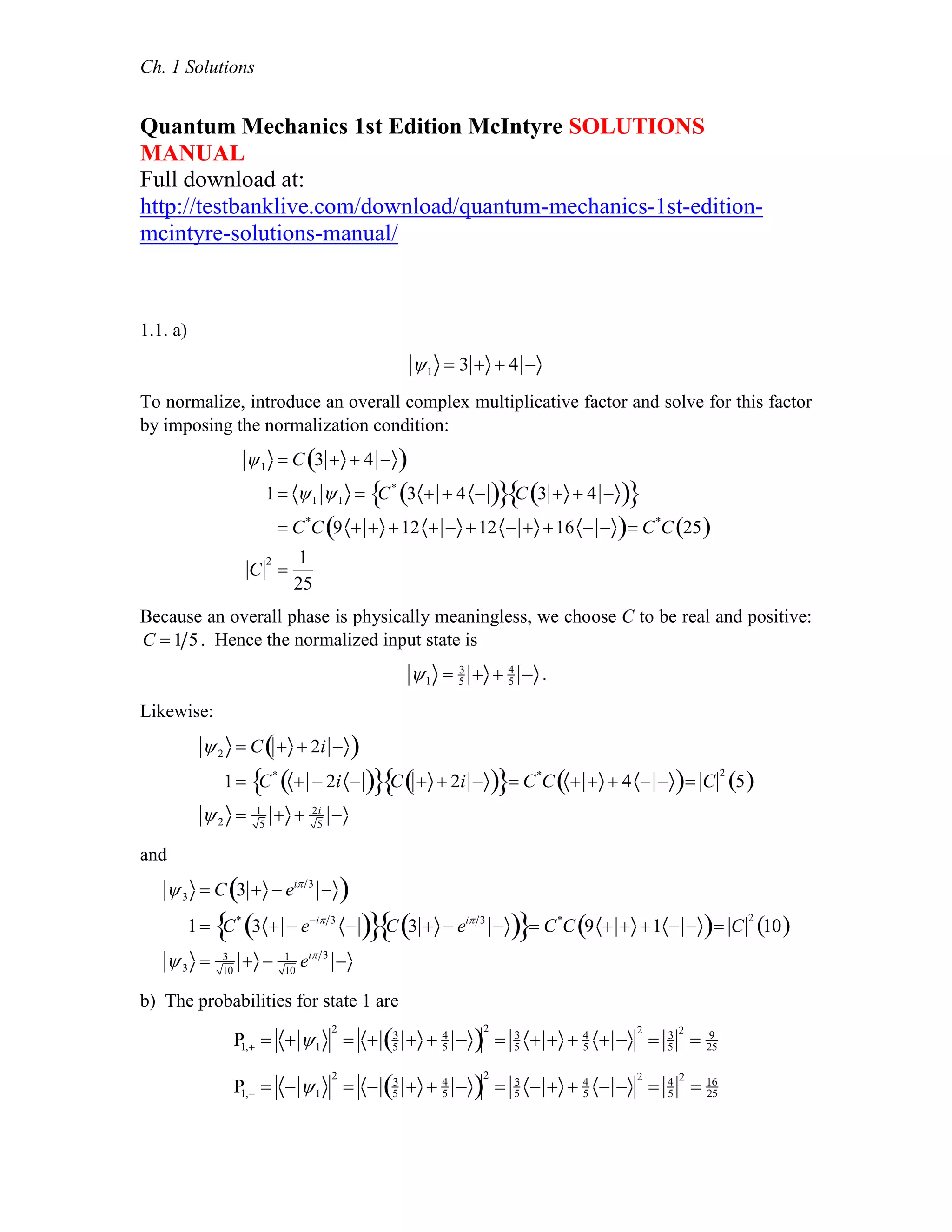
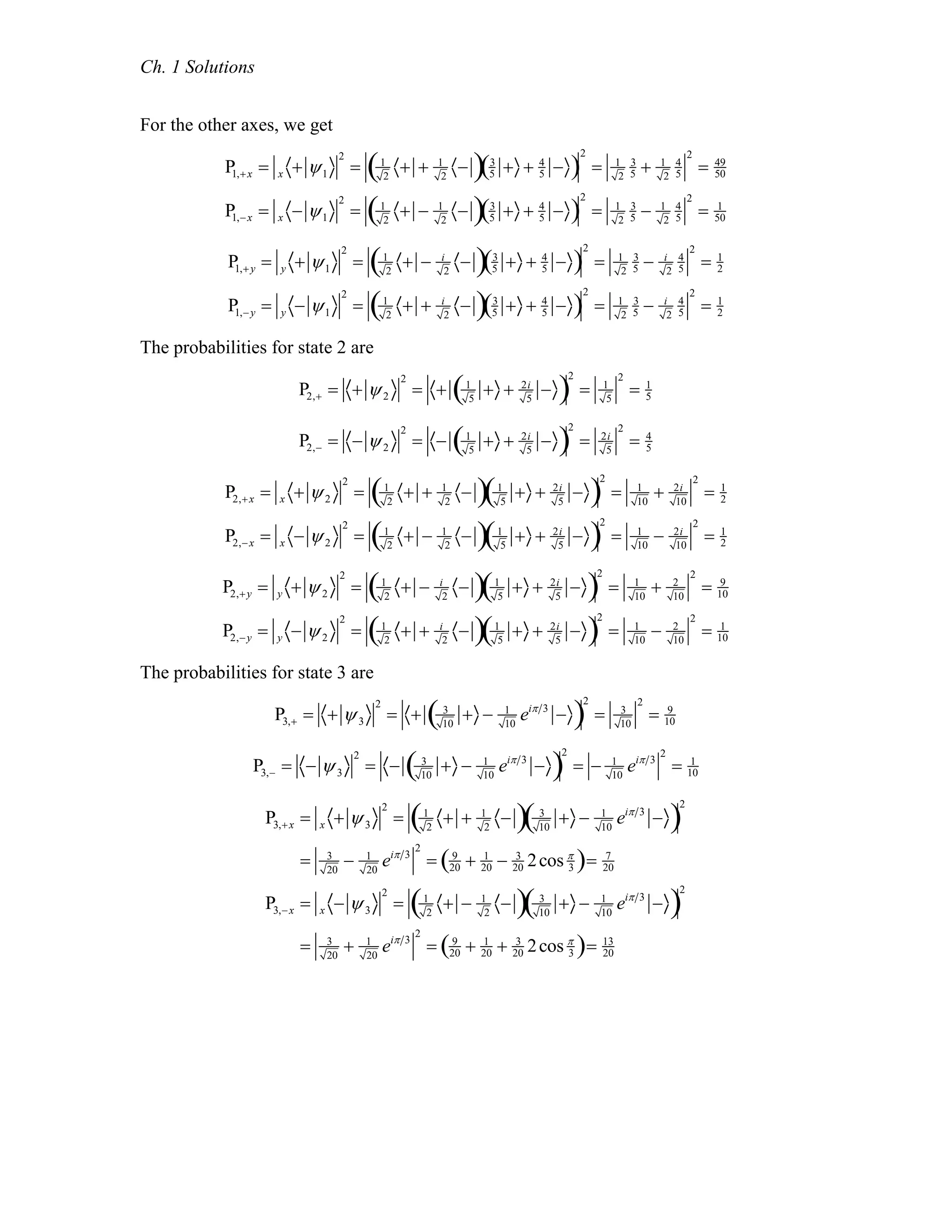
Ch. 1 Solutions
Quantum Mechanics 1st Edition McIntyre SOLUTIONS
MANUAL
Full download at:
http://testbanklive.com/download/quantum-mechanics-1st-edition-
mcintyre-solutions-manual/
1.1. a)
1  3   4 
To normalize, introduce an overall complex multiplicative factor and solve for this factor
by imposing the normalization condition:
1  C 3   4  
1 1 1  C*
3   4   C 3   4   
 C*
C 9   12   12   16    C*
C 25 
C
2

1
25
Because an overall phase is physically meaningless, we choose C to be real and positive:
C 1 5. Hence the normalized input state is
1  3
5   4
5  .
Likewise:
2  C   2i  
1 C*
  2i   C   2i    C*
C    4    C
2
5 
2  1
5
  2i
5

and
3  C 3   ei 3
 
1 C*
3   ei 3
  C 3   ei 3
   C*
C 9   1    C
2
10 
3  3
10
  1
10
ei 3

b) The probabilities for state 1 are
P1,   1
2
  3
5   4
5  
2
 3
5    4
5  
2
 3
5
2
 9
25
P1,   1
2
  3
5   4
5  
2
 3
5    4
5  
2
 4
5
2
 16
25
Ch. 1 Solutions
For the other axes, we get
P1,x  x  1
2
 1
2
  1
2
 3
5   4
5  
2
 1
2
3
5  1
2
4
5
2
 49
50
P1,x  x  1
2
 1
2
  1
2
 3
5   4
5  
2
 1
2
3
5  1
2
4
5
2
 1
50
P1,y  y  1
2
 1
2
  i
2
  3
5   4
5  
2
 1
2
3
5  i
2
4
5
2
 1
2
P1,y  y  1
2
 1
2
  i
2
  3
5   4
5  
2
 1
2
3
5  i
2
4
5
2
 1
2
The probabilities for state 2 are
P2,   2
2
  1
5
  2i
5
 
2
 1
5
2
 1
5
P2,   2
2
  1
5
  2i
5
 
2
 2i
5
2
 4
5
P2,x  x  2
2
 1
2
  1
2
  1
5
  2i
5
 
2
 1
10
 2i
10
2
 1
2
P2,x  x  2
2
 1
2
  1
2
  1
5
  2i
5
 
2
 1
10
 2i
10
2
 1
2
P2,y  y  2
2
 1
2
  i
2
  1
5
  2i
5
 
2
 1
10
 2
10
2
 9
10
P2,y  y  2
2
 1
2
  i
2
  1
5
  2i
5
 
2
 1
10
 2
10
2
 1
10
The probabilities for state 3 are
P3,   3
2
  3
10
  1
10
ei 3
 
2
 3
10
2
 9
10
P3,   3
2
  3
10
  1
10
ei 3
 
2
  1
10
ei 3
2
 1
10
P3,x  x  3
2
 1
2
  1
2
  3
10
  1
10
ei 3
 
2
 3
20
 1
20
ei 3
2
 9
20  1
20  3
20 2cos 
3  7
20
P3,x  x  3
2
 1
2
  1
2
  3
10
  1
10
ei 3
 
2
 3
20
 1
20
ei 3
2
 9
20  1
20  3
20 2cos 
3  13
20
Ch. 1 Solutions
P3,y  y  3
2
 1
2
  i
2
  3
10
  1
10
ei 3
 
2
 3
20
 i
20
ei 3
2
 9
20  1
20  3
20 2sin 
3  1
20 10  3 3  0.24
P3,y  y  3
2
 1
2
  i
2
  3
10
  1
10
ei 3
 
2
 3
20
 i
20
ei 3
2
 9
20  1
20  3
20 2sin 
3  1
20 10  3 3  0.76
c) Matrix notation:
1 B 1
5
3
4




2 B 1
5
1
2i




 3 B 1
10
3
ei 3






d) Probabilities in matrix notation
P1,   1
2
 1 0 1
5
3
4




2
 3
5
2
 9
25
P1,   1
2
 0 1 1
5
3
4




2
 4
5
2
 16
25
P1,x  x  1
2
 1
2 1 1 1
5
3
4




2
 1
2
3
5  1
2
4
5
2
 49
50
P1,x  x  1
2
 1
2 1 1 1
5
3
4




2
 1
2
3
5  1
2
4
5
2
 1
50
P1,y  y  1
2
 1
2 1 i 1
5
3
4




2
 1
2
3
5  i
2
4
5
2
 1
2
P1,y  y  1
2
 1
2 1 i 1
5
3
4




2
 1
2
3
5  i
2
4
5
2
 1
2
Ch. 1 Solutions
P2,   2
2
 1 0 1
5
1
2i




2
 1
5
2
 1
5
P2,   2
2
 0 1 1
5
1
2i




2
 2i
5
2
 4
5
P2,x  x  2
2
 1
2 1 1 1
5
1
2i




2
 1
10
 2i
10
2
 1
2
P2,x  x  2
2
 1
2 1 1 1
5
1
2i




2
 1
10
 2i
10
2
 1
2
P2,y  y  2
2
 1
2 1 i 1
5
1
2i




2
 1
10
 2
10
2
 9
10
P2,y  y  2
2
 1
2 1 i 1
5
1
2i




2
 1
10
 2
10
2
 1
10
P3,   3
2
 1 0 1
10
3
ei 3






2
 3
10
2
 9
10
P3,   3
2
 0 1 1
10
3
ei 3






2
 ei 3
10
2
 1
10
P3,x  x  3
2
 1
2 1 1 1
10
3
ei 3






2
 3
20
 1
20
ei 3
2
 7
20
P3,x  x  3
2
 1
2 1 1 1
10
3
ei 3






2
 3
20
 1
20
ei 3
2
 13
20
P3,y  y  3
2
 1
2 1 i 1
10
3
ei 3






2
 3
20
 i
20
ei 3
2
 1
20 10  3 3  0.24
P3,y  y  3
2
 1
2 1 i 1
10
3
ei 3






2
 3
20
 i
20
ei 3
2
 1
20 10  3 3  0.76
Ch. 1 Solutions
1.2 a)
State 1
1  1
3
  i 2
3

1  a   b 
1 1  0  a*
  b*
  1
3
  i 2
3
  0
a* 1
3
 ib* 2
3
 0  a*
 ib*
2
a
2
 b
2
 1  a
2

a
2
2  1  a  2
3
1  2
3
  i 1
3

State 2
2  1
5
  2
5

2  a   b 
2 2  0  a*
  b*
  1
5
  2
5
  0
a* 1
5
 b* 2
5
 0  a*
 b*
2
a
2
 b
2
 1  a
2

a
2
4  1  a  2
5
2  2
5
  1
5

State 3
3  1
2
  ei 4 1
2

3  a   b 
3 3  0  a*
  b*
  1
2
  ei 4 1
2
  0
a* 1
2
 ei 4
b* 1
2
 0  a*
 ei 4
b*
 b  aei 4
a
2
 b
2
 1  a
2
 a
2
 1  a  1
2
3  1
2
  ei 4 1
2

b) Inner products
Ch. 1 Solutions
1 1  1
3
  i 2
3
  1
3
  i 2
3
  1
3  2
3  1
1 2  1
3
  i 2
3
  1
5
  2
5
  1
15
 2 2i
15
 1
15
1 i2 2 
1 3  1
3
  i 2
3
  1
2
  ei 4
2
  1
6
 2iei 4
6
 1
6
2  i 
2 1  1
5
  2
5
  1
3
  i 2
3
  1
15
 2i
15
 1
15
1 i2 2 
2 2  1
5
  2
5
  1
5
  2
5
  1
5  4
5  1
2 3  1
5
  2
5
  1
2
  ei 4
2
  1
10
 2ei 4
10
 1
10
1 2  i 2 
3 1  1
2
  ei 4
2
  1
3
  i 2
3
  1
6
 2iei 4
6
 1
6
2  i 
3 2  1
2
  ei 4
2
  1
5
  2
5
  1
10
 2ei 4
10
 1
10
1 2  i 2 
3 3  1
2
  ei 4
2
  1
2
  ei 4
2
  1
2  1
2  1
1.3 Probability of measuring an in state  is
Pan
 an 
2
Probability of same measurement if state is changed to ei
 is
Pan ,NEW  an ei

2
 ei
an 
2
 an 
2
So the probability is unchanged.
1.4
 x
 a   b 
 x
 c   d 
P1,x  x  
2
 1
2
P2,x  x  
2
 1
2
P2,x  x  
2
 1
2
P1,x  x  
2
 c*
  d*
 
2
 c* 2
 c
2
 c
2
 1
2
P2,x  x  
2
 a*
  b*
 
2
 b* 2
 b
2
 b
2
 1
2
P2,x  x  
2
 c*
  d*
 
2
 d* 2
 d
2
 d
2
 1
2
Ch. 1 Solutions
1.5 a) Possible results of a measurement of the spin component Sz are always h 2 for a
spin-½ particle. Probabilities are
Ph 2   
2
  2
13
  i 3
13
 
2
 2
13
2
 4
13
Ph 2   
2
  2
13
  i 3
13
 
2
 3i
13
2
 9
13
b) Possible results of a measurement of the spin component Sx are always h 2 for a
spin-½ particle. Probabilities are
Px  x  
2
 1
2
  1
2
  2
13
  i 3
13
 
2
 2
26
 i 3
26
2
 1
2
Px  x  
2
 1
2
  1
2
  2
13
  i 3
13
 
2
 2
26
 i 3
26
2
 1
2
c) Histogram:
1.6 a) Possible results of a measurement of the spin component Sz are always h 2 for a
spin-½ particle. Probabilities are
Ph 2   
2
  2
13
 x
 i 3
13
 x 
2
 2
26
 i 3
26
2
 1
2
Ph 2   
2
  2
13
 x
 i 3
13
 x 
2
 2
26
 i 3
26
2
 1
2
b) Possible results of a measurement of the spin component Sx are always h 2 for a
spin-½ particle. Probabilities are
Px  x  
2
 x  2
13
 x
 i 3
13
 x 
2
 2
13
2
 4
13
Px  x  
2
 x  2
13
 x
 i 3
13
 x 
2
 3i
13
2
 9
13
Ch. 1 Solutions
c) Histogram:
1.7 a) Heads or tails: H or T
b) Each result is equally likely so
PH  1
2
PT  1
2
c) Histogram:
1.8 a) Six sides with 1, 2, 3, 4, 5, or 6 dots.
b) Each result is equally likely so
P1  P2  P3  P4  P5  P6  1
6
c) Histogram:
Ch. 1 Solutions
1.9 a) 36 possible die combinations with 11 possible numerical results:
2  11
3  1 2,2 1
4  1 3,2  2,31
5  1 4,2  3,3 2,4 1
6  1 5,2  4,3 3,4  2,5 1
7  1 6,2  5,3 4,4  3,5  2,6 1
8  2  6,3 5,4  4,5  3,6  2
9  3 6,4  5,5  4,6  3
10  4  6,5  5,6  4
11 5  6,6  5
12  6  6
b) Each possible die combination is equally likely, so the probabilities of the
numerical results are the number of possible combinations divided by 36:
P2  1
36 , P3  2
36  1
18 , P4  3
36  1
12 , P5  4
36  1
9 , P6  5
36 , P7  6
36  1
6 ,
P8  5
36 , P9  4
36  1
9 , P10  3
36  1
12 , P11  2
36  1
18 , P12  1
36
Note that the sum of the probabilities is unity as it must be.
c) Histogram:
1.10 a) The probabilities for state 1 are
P1,   1
2
  4
5   i 3
5  
2
 4
5
2
 16
25
P1,   1
2
  4
5   i 3
5  
2
 i 3
5
2
 9
25
P1,x  x  1
2
 1
2
  1
2
 4
5   i 3
5  
2
 1
2
4
5  i
2
3
5
2
 1
2
P1,x  x  1
2
 1
2
  1
2
 4
5   i 3
5  
2
 1
2
4
5  i
2
3
5
2
 1
2
P1,y  y  1
2
 1
2
  i
2
 4
5   i 3
5  
2
 1
2
4
5  1
2
3
5
2
 49
50
P1,y  y  1
2
 1
2
  i
2
 4
5   i 3
5  
2
 1
2
4
5  1
2
3
5
2
 1
50
Ch. 1 Solutions
The probabilities for state 2 are
P2,   2
2
  4
5   i 3
5  
2
 4
5
2
 16
25
P2,   2
2
  4
5   i 3
5  
2
 i 3
5
2
 9
25
P2,x  x  2
2
 1
2
  1
2
 4
5   i 3
5  
2
 1
2
4
5  i
2
3
5
2
 1
2
P2,x  x  2
2
 1
2
  1
2
 4
5   i 3
5  
2
 1
2
4
5  i
2
3
5
2
 1
2
P2,y  y  2
2
 1
2
  i
2
 4
5   i 3
5  
2
 1
2
4
5  1
2
3
5
2
 1
50
P2,y  y  2
2
 1
2
  i
2
 4
5   i 3
5  
2
 1
2
4
5  1
2
3
5
2
 49
50
The probabilities for state 3 are
P3,   3
2
   4
5   i 3
5  
2
  4
5
2
 16
25
P3,   3
2
   4
5   i 3
5  
2
 i 3
5
2
 9
25
P3,x  x  3
2
 1
2
  1
2
  4
5   i 3
5  
2
  1
2
4
5  i
2
3
5
2
 1
2
P3,x  x  3
2
 1
2
  1
2
  4
5   i 3
5  
2
  1
2
4
5  i
2
3
5
2
 1
2
P3,y  y  3
2
 1
2
  i
2
  4
5   i 3
5  
2
  1
2
4
5  1
2
3
5
2
 1
50
P3,y  y  3
2
 1
2
  i
2
  4
5   i 3
5  
2
  1
2
4
5  1
2
3
5
2
 49
50
b) States 2 and 3 differ only by an overall phase of ei
 1, so the measurement results
are the same; the states are physically indistinguishable. States 1 and 2 have different
relative phases between the coefficients, so they produce different results.
1.11 a) Possible results of a measurement of the spin component Sz are always h 2 for
a spin-½ particle. Probabilities are
Ph 2   
2
  3
34
  i 5
34
 
2
 3
34
2
 9
34  0.26
Ph 2   
2
  3
34
  i 5
34
 
2
 i 5
34
2
 25
34  0.74
b) After the measurement result of the spin component Sz is h 2 , the system is in the
 eigenstate corresponding to that result. The possible results of a measurement of the
spin component Sx are always h 2 for a spin-½ particle. The probabilities are
Px  x  after
2
 x  
2
 1
2
  1
2
 
2
 1
2
2
 1
2
Px  x  after
2
 x  
2
 1
2
  1
2
 
2
  1
2
2
 1
2
Ch. 1 Solutions
c) Diagrams
1.12 For a system with three possible measurement results: a1, a2, and a3, the three
eigenstates are a1 , a2 , and a3
Orthogonality:
a1 a2  0
a1 a3  0
a2 a3  0
Normalization:
a1 a1  1
a2 a2  1
a3 a3  1
Completeness:
  c1 a1  c2 a2  c3 a3
1.13 a) For a system with three possible measurement results: a1, a2, and a3, the three
eigenstates a1 , a2 , and a3 are
a1 B
1
0
0








a2 B
0
1
0








a3 B
0
0
1








Ch. 1 Solutions
b) In matrix notation, the state is
 B
1
2
5








The state given is not normalized, so first we normalize it:
  C
1
2
5








1    C*
1 2 5 C
1
2
5








 C*
C 1 4  25  1  C  1 30
The probabilities are
Pa1
 a1 
2
 1 0 0  1
30
1
2
5








2
 1
30
2
 1
30
Pa2
 a2 
2
 0 1 0  1
30
1
2
5








2
  2
30
2
 4
30
Pa3
 a3 
2
 0 0 1  1
30
1
2
5








2
 5
30
2
 25
30
Histogram:
c) In matrix notation, the state is
 B
2
3i
0








Ch. 1 Solutions
The state given is not normalized, so first we normalize it:
  C
2
3i
0








   C*
2 3i 0 C
2
3i
0








 C*
C 4  9  0  1  C  1 13
The probabilities are
Pa1
 a1 
2
 1 0 0 1
13
2
3i
0








2
 2
13
2
 4
13
Pa2
 a2 
2
 0 1 0 1
13
2
3i
0








2
 3i
13
2
 9
13
Pa3
 a3 
2
 0 0 1 1
13
2
3i
0








2
 0
13
2
 0
Histogram:
1.14. There are four possible measurement results: 2 eV, 4 eV, 7 eV, and 9 eV. The
probabilities are
P2 eV  2 eV 
2
 2 eV
1
39
3 2 eV  i 4 eV  2ei 7
7 eV  5 9 eV 
2
 9
39
P4 eV  4 eV 
2
 4 eV
1
39
3 2 eV  i 4 eV  2ei 7
7 eV  5 9 eV 
2
 1
39
Ch. 1 Solutions
P7 eV  7 eV 
2
 2 eV
1
39
3 2 eV  i 4 eV  2ei 7
7 eV  5 9 eV 
2
 4
39
P9 eV  9 eV 
2
 2 eV
1
39
3 2 eV  i 4 eV  2ei 7
7 eV  5 9 eV 
2
 25
39
Histogram:
1.15 The probability is
P f
  f i
2
 1i
3
a1  1
6
a2  1
6
a3  i
3
a1  2
3 a2 
2
 i
3
1i
3
 2
3
1
6
2
 i
3  1
3  1
3
2
 1
9  4
9  5
9
1.16 The measured probabilities are
P  1
2 Px  3
4 Py  0.067
P  1
2 Px  1
4 Py  0.933
Write the input state as
  a   b 
Equating the predicted Sz probabilities and the experimental results gives
P   
2
  a   b  
2
 a
2
 1
2  a  1
2
P   
2
  a   b  
2
 b
2
 1
2  b  1
2
ei
allowing for a possible relative phase. Equating the predicted Sx probabilities and the
experimental results gives
Px  x  
2
 1
2
   1
2
  ei
 
2
 1
2 1 ei
 
2
 1
4 1 ei
 1 ei
  1
4 11 ei
 ei
  1
2 1 cos  3
4
cos  1
2    
3 or 5
3
Ch. 1 Solutions
Equating the predicted Sy probabilities and the experimental results gives
Py  y  
2
 1
2
  i  1
2
  ei
 
2
 1
2 1 iei
 
2
 1
4 1 iei
 1 iei
  1
4 11 iei
 iei
  1
2 1 sin  0.067
sin  0.866    4
3 or 5
3    5
3
Hence the input state is
  1
2
  e
i5
3
   ˆn 
2
, 5
3 
1.17 Follow the solution method given in the lab handout. (i) For unknown number 1,
the measured probabilities are
P 1 Px  1
2 Py  1
2
P  0 Px  1
2 Py  1
2
Write the unknown state as
1  a   b 
Equating the predicted Sz probabilities and the experimental results gives
P   1
2
  a   b  
2
 a
2
1  a 1
P   1
2
  a   b  
2
 b
2
 0  b  0
Hence the unknown state is
1  
which produces the probabilities
P   1
2
  
2
 1
P   1
2
 1 
2
 0
Px  x  1
2
 1
2
  1
2
 
2
 1
2
Px  x  1
2
 1
2
  1
2
 
2
 1
2
Py  y  1
2
 1
2
  i
2
 
2
 1
2
Py  y  1
2
 1
2
  i
2
 
2
 1
2
in agreement with the experiment.
Ch. 1 Solutions
(ii) For unknown number 2, the measured probabilities are
P  1
2 Px  1
2 Py  0
P  1
2 Px  1
2 Py 1
Write the unknown state as
2  a  b 
Equating the predicted Sz probabilities and the experimental results gives
P   2
2
  a   b  
2
 a
2
 1
2  a  1
2
P   2
2
  a   b  
2
 b
2
 1
2  b  1
2
ei
allowing for a possible relative phase. Equating the predicted Sx probabilities and the
experimental results gives
Px  x  2
2
 1
2
   1
2
  ei
 
2
 1
2 1 ei
 
2
 1
4 1 ei
 1 ei
  1
4 11 ei
 ei
  1
2 1 cos  1
2
cos  0    
2 or 3
2
Equating the predicted Sy probabilities and the experimental results gives
Py  y  2
2
 1
2
  i  1
2
  ei
 
2
 1
2 1 iei
 
2
 1
4 1 iei
 1 iei
  1
4 11 iei
 iei
  1
2 1 sin  0
sin  1    3
2
Hence the unknown state is
2  1
2
  e
i 3
2
  1
2
  i    y
which produces the probabilities
P   2
2
  1
2
  i  
2
 1
2
P   2
2
  1
2
  i  
2
 1
2
Px  x  2
2
 1
2
   1
2
  i  
2
 1
2
Px  x  2
2
 1
2
   1
2
  i  
2
 1
2
Py  y  2
2
 1
2
  i  1
2
  i  
2
 0
Py  y  2
2
 1
2
  i  1
2
  i  
2
 1
Ch. 1 Solutions
in agreement with the experiment.
(iii) For unknown number 3, the measured probabilities are
P  1
2 Px  1
4 Py  0.067
P  1
2 Px  3
4 Py  0.933
Write the unknown state as
3  a  b 
Equating the predicted Sz probabilities and the experimental results gives
P   3
2
  a   b  
2
 a
2
 1
2  a  1
2
P   3
2
  a   b  
2
 b
2
 1
2  b  1
2
ei
allowing for a possible relative phase. Equating the predicted Sx probabilities and the
experimental results gives
Px  x  3
2
 1
2
   1
2
  ei
 
2
 1
2 1 ei
 
2
 1
4 1 ei
 1 ei
  1
4 11 ei
 ei
  1
2 1 cos  1
4
cos   1
2    2
3 or 4
3
Equating the predicted Sy probabilities and the experimental results gives
Py  y  3
2
 1
2
  i  1
2
  ei
 
2
 1
2 1 iei
 
2
 1
4 1 iei
 1 iei
  1
4 11 iei
 iei
  1
2 1 sin  0.067
sin  0.866    4
3 or 5
3    4
3
Hence the unknown state is
3  1
2
  e
i 4
3
   ˆn 
2
,  4
3 
which produces the probabilities
P   3
2
  1
2
  e
i 4 
3
 
2
 1
2
P   3
2
  1
2
  e
i 4 
3
 
2
 1
2
Px  x  3
2
 1
2
   1
2
  e
i 4 
3
 
2
 1
2 1 cos 4
3  1
4
Px  x  3
2
 1
2
   1
2
  e
i 4 
3
 
2
 1
2 1 cos 4
3  3
4
Ch. 1 Solutions
Py  y  3
2
 1
2
  i  1
2
  e
i 4 
3
 
2
 1
2 1 sin 4
3  1
2 1 3
2  0.067
Py  y  3
2
 1
2
  i  1
2
  e
i 4 
3
 
2
 1
2 1 sin 4
3  1
2 1 3
2  0.933
in agreement with the experiment.
(iv) For unknown number 4, the measured probabilities are
P  1
4 Px  7
8 Py  0.283
P  3
4 Px  1
8 Py  0.717
Write the unknown state as
4  a   b 
Equating the predicted Sz probabilities and the experimental results gives
P   4
2
  a   b  
2
 a
2
 1
4  a  1
2
P   4
2
  a   b  
2
 b
2
 3
4  b  3
2 ei
allowing for a possible relative phase. Equating the predicted Sx probabilities and the
experimental results gives
Px  x  4
2
 1
2
   1
2   3ei
 
2
 1
2 2
1 3ei
 
2
 1
8 1 3ei
 1 3ei
  1
8 1 3 3ei
 3ei
  1
4 2  3cos  7
8
cos  3
2    
6 or 11
6
Equating the predicted Sy probabilities and the experimental results gives
Py  y  4
2
 1
2
  i  1
2   3ei
 
2
 1
2 2
1 i 3ei
 
2
 1
8 1 i 3ei
 1 i 3ei
  1
8 1 3 i 3ei
 i 3ei
  1
4 2  3sin  0.283
sin  0.50    7
6 or 11
6    11
6
Hence the unknown state is
4  1
2   3
2 e
i11
6
  cos 
3   sin 
3 e
i11
6
   ˆn 2
3
, 11
6 
which produces the probabilities
Ch. 1 Solutions
P   4
2
  1
2   3e
i11
6
 
2
 1
4
P   4
2
  1
2   3e
i11
6
 
2
 3
4
Px  x  4
2
 1
2
   1
2   3e
i11
6
 
2
 1
4 2  3cos11
6  7
8
Px  x  4
2
 1
2
   1
2   3e
i11
6
 
2
 1
4 2  3cos11
6  1
8
Py  y  4
2
 1
2
  i  1
2   3e
i11
6
 
2
 1
4 2  3sin 11
6  1
4 2  3
2  0.283
Py  y  4
2
 1
2
  i  1
2   3e
i11
6
 
2
 1
4 2  3sin 11
6  1
4 2  3
2  0.717
in agreement with the experiment.
Quantum Mechanics 1st Edition McIntyre SOLUTIONS
MANUAL
Full download at:
http://testbanklive.com/download/quantum-mechanics-1st-edition-
mcintyre-solutions-manual/
quantum mechanics david mcintyre solutions pdf
quantum mechanics mcintyre pdf
quantum mechanics a paradigms approach solutions pdf
quantum mechanics mcintyre solutions pdf
quantum mechanics a paradigms approach solution manual
quantum mechanics mcintyre solutions manual pdf
hidden life of prayer

Quantum mechanics 1st edition mc intyre solutions manual

  • 1.
    Ch. 1 Solutions QuantumMechanics 1st Edition McIntyre SOLUTIONS MANUAL Full download at: http://testbanklive.com/download/quantum-mechanics-1st-edition- mcintyre-solutions-manual/ 1.1. a) 1  3   4  To normalize, introduce an overall complex multiplicative factor and solve for this factor by imposing the normalization condition: 1  C 3   4   1 1 1  C* 3   4   C 3   4     C* C 9   12   12   16    C* C 25  C 2  1 25 Because an overall phase is physically meaningless, we choose C to be real and positive: C 1 5. Hence the normalized input state is 1  3 5   4 5  . Likewise: 2  C   2i   1 C*   2i   C   2i    C* C    4    C 2 5  2  1 5   2i 5  and 3  C 3   ei 3   1 C* 3   ei 3   C 3   ei 3    C* C 9   1    C 2 10  3  3 10   1 10 ei 3  b) The probabilities for state 1 are P1,   1 2   3 5   4 5   2  3 5    4 5   2  3 5 2  9 25 P1,   1 2   3 5   4 5   2  3 5    4 5   2  4 5 2  16 25
  • 2.
    Ch. 1 Solutions Forthe other axes, we get P1,x  x  1 2  1 2   1 2  3 5   4 5   2  1 2 3 5  1 2 4 5 2  49 50 P1,x  x  1 2  1 2   1 2  3 5   4 5   2  1 2 3 5  1 2 4 5 2  1 50 P1,y  y  1 2  1 2   i 2   3 5   4 5   2  1 2 3 5  i 2 4 5 2  1 2 P1,y  y  1 2  1 2   i 2   3 5   4 5   2  1 2 3 5  i 2 4 5 2  1 2 The probabilities for state 2 are P2,   2 2   1 5   2i 5   2  1 5 2  1 5 P2,   2 2   1 5   2i 5   2  2i 5 2  4 5 P2,x  x  2 2  1 2   1 2   1 5   2i 5   2  1 10  2i 10 2  1 2 P2,x  x  2 2  1 2   1 2   1 5   2i 5   2  1 10  2i 10 2  1 2 P2,y  y  2 2  1 2   i 2   1 5   2i 5   2  1 10  2 10 2  9 10 P2,y  y  2 2  1 2   i 2   1 5   2i 5   2  1 10  2 10 2  1 10 The probabilities for state 3 are P3,   3 2   3 10   1 10 ei 3   2  3 10 2  9 10 P3,   3 2   3 10   1 10 ei 3   2   1 10 ei 3 2  1 10 P3,x  x  3 2  1 2   1 2   3 10   1 10 ei 3   2  3 20  1 20 ei 3 2  9 20  1 20  3 20 2cos  3  7 20 P3,x  x  3 2  1 2   1 2   3 10   1 10 ei 3   2  3 20  1 20 ei 3 2  9 20  1 20  3 20 2cos  3  13 20
  • 3.
    Ch. 1 Solutions P3,y y  3 2  1 2   i 2   3 10   1 10 ei 3   2  3 20  i 20 ei 3 2  9 20  1 20  3 20 2sin  3  1 20 10  3 3  0.24 P3,y  y  3 2  1 2   i 2   3 10   1 10 ei 3   2  3 20  i 20 ei 3 2  9 20  1 20  3 20 2sin  3  1 20 10  3 3  0.76 c) Matrix notation: 1 B 1 5 3 4     2 B 1 5 1 2i      3 B 1 10 3 ei 3       d) Probabilities in matrix notation P1,   1 2  1 0 1 5 3 4     2  3 5 2  9 25 P1,   1 2  0 1 1 5 3 4     2  4 5 2  16 25 P1,x  x  1 2  1 2 1 1 1 5 3 4     2  1 2 3 5  1 2 4 5 2  49 50 P1,x  x  1 2  1 2 1 1 1 5 3 4     2  1 2 3 5  1 2 4 5 2  1 50 P1,y  y  1 2  1 2 1 i 1 5 3 4     2  1 2 3 5  i 2 4 5 2  1 2 P1,y  y  1 2  1 2 1 i 1 5 3 4     2  1 2 3 5  i 2 4 5 2  1 2
  • 4.
    Ch. 1 Solutions P2,  2 2  1 0 1 5 1 2i     2  1 5 2  1 5 P2,   2 2  0 1 1 5 1 2i     2  2i 5 2  4 5 P2,x  x  2 2  1 2 1 1 1 5 1 2i     2  1 10  2i 10 2  1 2 P2,x  x  2 2  1 2 1 1 1 5 1 2i     2  1 10  2i 10 2  1 2 P2,y  y  2 2  1 2 1 i 1 5 1 2i     2  1 10  2 10 2  9 10 P2,y  y  2 2  1 2 1 i 1 5 1 2i     2  1 10  2 10 2  1 10 P3,   3 2  1 0 1 10 3 ei 3       2  3 10 2  9 10 P3,   3 2  0 1 1 10 3 ei 3       2  ei 3 10 2  1 10 P3,x  x  3 2  1 2 1 1 1 10 3 ei 3       2  3 20  1 20 ei 3 2  7 20 P3,x  x  3 2  1 2 1 1 1 10 3 ei 3       2  3 20  1 20 ei 3 2  13 20 P3,y  y  3 2  1 2 1 i 1 10 3 ei 3       2  3 20  i 20 ei 3 2  1 20 10  3 3  0.24 P3,y  y  3 2  1 2 1 i 1 10 3 ei 3       2  3 20  i 20 ei 3 2  1 20 10  3 3  0.76
  • 5.
    Ch. 1 Solutions 1.2a) State 1 1  1 3   i 2 3  1  a   b  1 1  0  a*   b*   1 3   i 2 3   0 a* 1 3  ib* 2 3  0  a*  ib* 2 a 2  b 2  1  a 2  a 2 2  1  a  2 3 1  2 3   i 1 3  State 2 2  1 5   2 5  2  a   b  2 2  0  a*   b*   1 5   2 5   0 a* 1 5  b* 2 5  0  a*  b* 2 a 2  b 2  1  a 2  a 2 4  1  a  2 5 2  2 5   1 5  State 3 3  1 2   ei 4 1 2  3  a   b  3 3  0  a*   b*   1 2   ei 4 1 2   0 a* 1 2  ei 4 b* 1 2  0  a*  ei 4 b*  b  aei 4 a 2  b 2  1  a 2  a 2  1  a  1 2 3  1 2   ei 4 1 2  b) Inner products
  • 6.
    Ch. 1 Solutions 11  1 3   i 2 3   1 3   i 2 3   1 3  2 3  1 1 2  1 3   i 2 3   1 5   2 5   1 15  2 2i 15  1 15 1 i2 2  1 3  1 3   i 2 3   1 2   ei 4 2   1 6  2iei 4 6  1 6 2  i  2 1  1 5   2 5   1 3   i 2 3   1 15  2i 15  1 15 1 i2 2  2 2  1 5   2 5   1 5   2 5   1 5  4 5  1 2 3  1 5   2 5   1 2   ei 4 2   1 10  2ei 4 10  1 10 1 2  i 2  3 1  1 2   ei 4 2   1 3   i 2 3   1 6  2iei 4 6  1 6 2  i  3 2  1 2   ei 4 2   1 5   2 5   1 10  2ei 4 10  1 10 1 2  i 2  3 3  1 2   ei 4 2   1 2   ei 4 2   1 2  1 2  1 1.3 Probability of measuring an in state  is Pan  an  2 Probability of same measurement if state is changed to ei  is Pan ,NEW  an ei  2  ei an  2  an  2 So the probability is unchanged. 1.4  x  a   b   x  c   d  P1,x  x   2  1 2 P2,x  x   2  1 2 P2,x  x   2  1 2 P1,x  x   2  c*   d*   2  c* 2  c 2  c 2  1 2 P2,x  x   2  a*   b*   2  b* 2  b 2  b 2  1 2 P2,x  x   2  c*   d*   2  d* 2  d 2  d 2  1 2
  • 7.
    Ch. 1 Solutions 1.5a) Possible results of a measurement of the spin component Sz are always h 2 for a spin-½ particle. Probabilities are Ph 2    2   2 13   i 3 13   2  2 13 2  4 13 Ph 2    2   2 13   i 3 13   2  3i 13 2  9 13 b) Possible results of a measurement of the spin component Sx are always h 2 for a spin-½ particle. Probabilities are Px  x   2  1 2   1 2   2 13   i 3 13   2  2 26  i 3 26 2  1 2 Px  x   2  1 2   1 2   2 13   i 3 13   2  2 26  i 3 26 2  1 2 c) Histogram: 1.6 a) Possible results of a measurement of the spin component Sz are always h 2 for a spin-½ particle. Probabilities are Ph 2    2   2 13  x  i 3 13  x  2  2 26  i 3 26 2  1 2 Ph 2    2   2 13  x  i 3 13  x  2  2 26  i 3 26 2  1 2 b) Possible results of a measurement of the spin component Sx are always h 2 for a spin-½ particle. Probabilities are Px  x   2  x  2 13  x  i 3 13  x  2  2 13 2  4 13 Px  x   2  x  2 13  x  i 3 13  x  2  3i 13 2  9 13
  • 8.
    Ch. 1 Solutions c)Histogram: 1.7 a) Heads or tails: H or T b) Each result is equally likely so PH  1 2 PT  1 2 c) Histogram: 1.8 a) Six sides with 1, 2, 3, 4, 5, or 6 dots. b) Each result is equally likely so P1  P2  P3  P4  P5  P6  1 6 c) Histogram:
  • 9.
    Ch. 1 Solutions 1.9a) 36 possible die combinations with 11 possible numerical results: 2  11 3  1 2,2 1 4  1 3,2  2,31 5  1 4,2  3,3 2,4 1 6  1 5,2  4,3 3,4  2,5 1 7  1 6,2  5,3 4,4  3,5  2,6 1 8  2  6,3 5,4  4,5  3,6  2 9  3 6,4  5,5  4,6  3 10  4  6,5  5,6  4 11 5  6,6  5 12  6  6 b) Each possible die combination is equally likely, so the probabilities of the numerical results are the number of possible combinations divided by 36: P2  1 36 , P3  2 36  1 18 , P4  3 36  1 12 , P5  4 36  1 9 , P6  5 36 , P7  6 36  1 6 , P8  5 36 , P9  4 36  1 9 , P10  3 36  1 12 , P11  2 36  1 18 , P12  1 36 Note that the sum of the probabilities is unity as it must be. c) Histogram: 1.10 a) The probabilities for state 1 are P1,   1 2   4 5   i 3 5   2  4 5 2  16 25 P1,   1 2   4 5   i 3 5   2  i 3 5 2  9 25 P1,x  x  1 2  1 2   1 2  4 5   i 3 5   2  1 2 4 5  i 2 3 5 2  1 2 P1,x  x  1 2  1 2   1 2  4 5   i 3 5   2  1 2 4 5  i 2 3 5 2  1 2 P1,y  y  1 2  1 2   i 2  4 5   i 3 5   2  1 2 4 5  1 2 3 5 2  49 50 P1,y  y  1 2  1 2   i 2  4 5   i 3 5   2  1 2 4 5  1 2 3 5 2  1 50
  • 10.
    Ch. 1 Solutions Theprobabilities for state 2 are P2,   2 2   4 5   i 3 5   2  4 5 2  16 25 P2,   2 2   4 5   i 3 5   2  i 3 5 2  9 25 P2,x  x  2 2  1 2   1 2  4 5   i 3 5   2  1 2 4 5  i 2 3 5 2  1 2 P2,x  x  2 2  1 2   1 2  4 5   i 3 5   2  1 2 4 5  i 2 3 5 2  1 2 P2,y  y  2 2  1 2   i 2  4 5   i 3 5   2  1 2 4 5  1 2 3 5 2  1 50 P2,y  y  2 2  1 2   i 2  4 5   i 3 5   2  1 2 4 5  1 2 3 5 2  49 50 The probabilities for state 3 are P3,   3 2    4 5   i 3 5   2   4 5 2  16 25 P3,   3 2    4 5   i 3 5   2  i 3 5 2  9 25 P3,x  x  3 2  1 2   1 2   4 5   i 3 5   2   1 2 4 5  i 2 3 5 2  1 2 P3,x  x  3 2  1 2   1 2   4 5   i 3 5   2   1 2 4 5  i 2 3 5 2  1 2 P3,y  y  3 2  1 2   i 2   4 5   i 3 5   2   1 2 4 5  1 2 3 5 2  1 50 P3,y  y  3 2  1 2   i 2   4 5   i 3 5   2   1 2 4 5  1 2 3 5 2  49 50 b) States 2 and 3 differ only by an overall phase of ei  1, so the measurement results are the same; the states are physically indistinguishable. States 1 and 2 have different relative phases between the coefficients, so they produce different results. 1.11 a) Possible results of a measurement of the spin component Sz are always h 2 for a spin-½ particle. Probabilities are Ph 2    2   3 34   i 5 34   2  3 34 2  9 34  0.26 Ph 2    2   3 34   i 5 34   2  i 5 34 2  25 34  0.74 b) After the measurement result of the spin component Sz is h 2 , the system is in the  eigenstate corresponding to that result. The possible results of a measurement of the spin component Sx are always h 2 for a spin-½ particle. The probabilities are Px  x  after 2  x   2  1 2   1 2   2  1 2 2  1 2 Px  x  after 2  x   2  1 2   1 2   2   1 2 2  1 2
  • 11.
    Ch. 1 Solutions c)Diagrams 1.12 For a system with three possible measurement results: a1, a2, and a3, the three eigenstates are a1 , a2 , and a3 Orthogonality: a1 a2  0 a1 a3  0 a2 a3  0 Normalization: a1 a1  1 a2 a2  1 a3 a3  1 Completeness:   c1 a1  c2 a2  c3 a3 1.13 a) For a system with three possible measurement results: a1, a2, and a3, the three eigenstates a1 , a2 , and a3 are a1 B 1 0 0         a2 B 0 1 0         a3 B 0 0 1        
  • 12.
    Ch. 1 Solutions b)In matrix notation, the state is  B 1 2 5         The state given is not normalized, so first we normalize it:   C 1 2 5         1    C* 1 2 5 C 1 2 5          C* C 1 4  25  1  C  1 30 The probabilities are Pa1  a1  2  1 0 0  1 30 1 2 5         2  1 30 2  1 30 Pa2  a2  2  0 1 0  1 30 1 2 5         2   2 30 2  4 30 Pa3  a3  2  0 0 1  1 30 1 2 5         2  5 30 2  25 30 Histogram: c) In matrix notation, the state is  B 2 3i 0        
  • 13.
    Ch. 1 Solutions Thestate given is not normalized, so first we normalize it:   C 2 3i 0            C* 2 3i 0 C 2 3i 0          C* C 4  9  0  1  C  1 13 The probabilities are Pa1  a1  2  1 0 0 1 13 2 3i 0         2  2 13 2  4 13 Pa2  a2  2  0 1 0 1 13 2 3i 0         2  3i 13 2  9 13 Pa3  a3  2  0 0 1 1 13 2 3i 0         2  0 13 2  0 Histogram: 1.14. There are four possible measurement results: 2 eV, 4 eV, 7 eV, and 9 eV. The probabilities are P2 eV  2 eV  2  2 eV 1 39 3 2 eV  i 4 eV  2ei 7 7 eV  5 9 eV  2  9 39 P4 eV  4 eV  2  4 eV 1 39 3 2 eV  i 4 eV  2ei 7 7 eV  5 9 eV  2  1 39
  • 14.
    Ch. 1 Solutions P7eV  7 eV  2  2 eV 1 39 3 2 eV  i 4 eV  2ei 7 7 eV  5 9 eV  2  4 39 P9 eV  9 eV  2  2 eV 1 39 3 2 eV  i 4 eV  2ei 7 7 eV  5 9 eV  2  25 39 Histogram: 1.15 The probability is P f   f i 2  1i 3 a1  1 6 a2  1 6 a3  i 3 a1  2 3 a2  2  i 3 1i 3  2 3 1 6 2  i 3  1 3  1 3 2  1 9  4 9  5 9 1.16 The measured probabilities are P  1 2 Px  3 4 Py  0.067 P  1 2 Px  1 4 Py  0.933 Write the input state as   a   b  Equating the predicted Sz probabilities and the experimental results gives P    2   a   b   2  a 2  1 2  a  1 2 P    2   a   b   2  b 2  1 2  b  1 2 ei allowing for a possible relative phase. Equating the predicted Sx probabilities and the experimental results gives Px  x   2  1 2    1 2   ei   2  1 2 1 ei   2  1 4 1 ei  1 ei   1 4 11 ei  ei   1 2 1 cos  3 4 cos  1 2     3 or 5 3
  • 15.
    Ch. 1 Solutions Equatingthe predicted Sy probabilities and the experimental results gives Py  y   2  1 2   i  1 2   ei   2  1 2 1 iei   2  1 4 1 iei  1 iei   1 4 11 iei  iei   1 2 1 sin  0.067 sin  0.866    4 3 or 5 3    5 3 Hence the input state is   1 2   e i5 3    ˆn  2 , 5 3  1.17 Follow the solution method given in the lab handout. (i) For unknown number 1, the measured probabilities are P 1 Px  1 2 Py  1 2 P  0 Px  1 2 Py  1 2 Write the unknown state as 1  a   b  Equating the predicted Sz probabilities and the experimental results gives P   1 2   a   b   2  a 2 1  a 1 P   1 2   a   b   2  b 2  0  b  0 Hence the unknown state is 1   which produces the probabilities P   1 2    2  1 P   1 2  1  2  0 Px  x  1 2  1 2   1 2   2  1 2 Px  x  1 2  1 2   1 2   2  1 2 Py  y  1 2  1 2   i 2   2  1 2 Py  y  1 2  1 2   i 2   2  1 2 in agreement with the experiment.
  • 16.
    Ch. 1 Solutions (ii)For unknown number 2, the measured probabilities are P  1 2 Px  1 2 Py  0 P  1 2 Px  1 2 Py 1 Write the unknown state as 2  a  b  Equating the predicted Sz probabilities and the experimental results gives P   2 2   a   b   2  a 2  1 2  a  1 2 P   2 2   a   b   2  b 2  1 2  b  1 2 ei allowing for a possible relative phase. Equating the predicted Sx probabilities and the experimental results gives Px  x  2 2  1 2    1 2   ei   2  1 2 1 ei   2  1 4 1 ei  1 ei   1 4 11 ei  ei   1 2 1 cos  1 2 cos  0     2 or 3 2 Equating the predicted Sy probabilities and the experimental results gives Py  y  2 2  1 2   i  1 2   ei   2  1 2 1 iei   2  1 4 1 iei  1 iei   1 4 11 iei  iei   1 2 1 sin  0 sin  1    3 2 Hence the unknown state is 2  1 2   e i 3 2   1 2   i    y which produces the probabilities P   2 2   1 2   i   2  1 2 P   2 2   1 2   i   2  1 2 Px  x  2 2  1 2    1 2   i   2  1 2 Px  x  2 2  1 2    1 2   i   2  1 2 Py  y  2 2  1 2   i  1 2   i   2  0 Py  y  2 2  1 2   i  1 2   i   2  1
  • 17.
    Ch. 1 Solutions inagreement with the experiment. (iii) For unknown number 3, the measured probabilities are P  1 2 Px  1 4 Py  0.067 P  1 2 Px  3 4 Py  0.933 Write the unknown state as 3  a  b  Equating the predicted Sz probabilities and the experimental results gives P   3 2   a   b   2  a 2  1 2  a  1 2 P   3 2   a   b   2  b 2  1 2  b  1 2 ei allowing for a possible relative phase. Equating the predicted Sx probabilities and the experimental results gives Px  x  3 2  1 2    1 2   ei   2  1 2 1 ei   2  1 4 1 ei  1 ei   1 4 11 ei  ei   1 2 1 cos  1 4 cos   1 2    2 3 or 4 3 Equating the predicted Sy probabilities and the experimental results gives Py  y  3 2  1 2   i  1 2   ei   2  1 2 1 iei   2  1 4 1 iei  1 iei   1 4 11 iei  iei   1 2 1 sin  0.067 sin  0.866    4 3 or 5 3    4 3 Hence the unknown state is 3  1 2   e i 4 3    ˆn  2 ,  4 3  which produces the probabilities P   3 2   1 2   e i 4  3   2  1 2 P   3 2   1 2   e i 4  3   2  1 2 Px  x  3 2  1 2    1 2   e i 4  3   2  1 2 1 cos 4 3  1 4 Px  x  3 2  1 2    1 2   e i 4  3   2  1 2 1 cos 4 3  3 4
  • 18.
    Ch. 1 Solutions Py y  3 2  1 2   i  1 2   e i 4  3   2  1 2 1 sin 4 3  1 2 1 3 2  0.067 Py  y  3 2  1 2   i  1 2   e i 4  3   2  1 2 1 sin 4 3  1 2 1 3 2  0.933 in agreement with the experiment. (iv) For unknown number 4, the measured probabilities are P  1 4 Px  7 8 Py  0.283 P  3 4 Px  1 8 Py  0.717 Write the unknown state as 4  a   b  Equating the predicted Sz probabilities and the experimental results gives P   4 2   a   b   2  a 2  1 4  a  1 2 P   4 2   a   b   2  b 2  3 4  b  3 2 ei allowing for a possible relative phase. Equating the predicted Sx probabilities and the experimental results gives Px  x  4 2  1 2    1 2   3ei   2  1 2 2 1 3ei   2  1 8 1 3ei  1 3ei   1 8 1 3 3ei  3ei   1 4 2  3cos  7 8 cos  3 2     6 or 11 6 Equating the predicted Sy probabilities and the experimental results gives Py  y  4 2  1 2   i  1 2   3ei   2  1 2 2 1 i 3ei   2  1 8 1 i 3ei  1 i 3ei   1 8 1 3 i 3ei  i 3ei   1 4 2  3sin  0.283 sin  0.50    7 6 or 11 6    11 6 Hence the unknown state is 4  1 2   3 2 e i11 6   cos  3   sin  3 e i11 6    ˆn 2 3 , 11 6  which produces the probabilities
  • 19.
    Ch. 1 Solutions P  4 2   1 2   3e i11 6   2  1 4 P   4 2   1 2   3e i11 6   2  3 4 Px  x  4 2  1 2    1 2   3e i11 6   2  1 4 2  3cos11 6  7 8 Px  x  4 2  1 2    1 2   3e i11 6   2  1 4 2  3cos11 6  1 8 Py  y  4 2  1 2   i  1 2   3e i11 6   2  1 4 2  3sin 11 6  1 4 2  3 2  0.283 Py  y  4 2  1 2   i  1 2   3e i11 6   2  1 4 2  3sin 11 6  1 4 2  3 2  0.717 in agreement with the experiment. Quantum Mechanics 1st Edition McIntyre SOLUTIONS MANUAL Full download at: http://testbanklive.com/download/quantum-mechanics-1st-edition- mcintyre-solutions-manual/ quantum mechanics david mcintyre solutions pdf quantum mechanics mcintyre pdf quantum mechanics a paradigms approach solutions pdf quantum mechanics mcintyre solutions pdf quantum mechanics a paradigms approach solution manual quantum mechanics mcintyre solutions manual pdf hidden life of prayer