This paper presents an optimal computational algorithm for solution matrices of single-delay linear neutral scalar differential equations, establishing expressions based on a five-fold delay horizon. The methodology leverages continuity, change of variables, and linear difference theories to create solution matrices for various intervals. The findings contribute to the understanding and application of these solution matrices in real-world differential equation scenarios.

1. International Journal of Mathematics and Statistics Invention (IJMSI)
E-ISSN: 2321 – 4767 P-ISSN: 2321 - 4759
www.ijmsi.org Volume 2 Issue 8 || August. 2014 || PP-36-46
www.ijmsi.org 36 | P a g e
On optimal computational algorithm and transition cardinalities
for solution matrices of single–delaylinear neutral scalar
differential equations.
Ukwu Chukwunenye
Department of Mathematics University of Jos P.M.B 2084 Jos, Nigeria
ABSTRACT : This paper established an optimal computationalalgorithm for solution matrices of single–delay
autonomous linear neutral equations based on the established expressions of such matrices on a horizon of
length equal to five times the delay. The development of the solution matrices exploited the continuity of these
matrices for positive time periods, the method of steps, change of variablesand theory of linear difference
equations to obtain these matrices on successive intervals of length equal to the delay h.
KEYWORDS: Algorithm, Equations, Matrices, Neutral, Solution.
I. INTRODUCTION
Solution matrices are integral components of variation of constants formulas in the computations of
solutions of linear and perturbed linear functional differential equations, Ukwu [1]. But quite curiously, no
other author has made any serious attemptto investigate the existence or otherwise of their general expressions
for various classes of these equations. Effort has usually focused on the single – delay model and the approach
has been to start from the interval [0,h] , compute the solution matrices and solutions for given problem
instances and then use the method of steps to extend these to the intervals [kh, (k 1)h], for positive
integral k , not exceeding 2, for the most part. Such approach is rather restrictive and doomed to failure in terms
of structure for arbitrary k . In other words such approach fails to address the issue of the structure of solution
matrices and solutions quite vital for real-world applications.With a view to addressing such short-comings,
Ukwu and Garba[2] blazed the trail by consideringthe class of double – delay scalar differential equations:
x(t)  ax(t) bx(t  h)  cx(t  2h), t R,
where a, b and c are arbitrary real constants. By deploying ingenious combinations of summation notations,
multinomial distribution, greatest integer functions, change of variables techniques, multiple integrals, as well as
the method of steps, the paperderived the following optimal expressions for the solution matrices:
 
   
0
2 2
( ) [ 2 ] )
1 1 0
, ;
( )
[ 2 ] ; , 1
! ! !
at
k
i k j i j k
at i a t ih i j a t i j h
k
i j i
e t J
Y t
t ih b c
e b e t i j h e t J k
i i j
 
    
   
  
 

  
      

  
where [ , ( 1) ], {0,1, },   denotes the greatest integer function, and ( ) denotes a generic
solution matrix of the above class of equations for . See also [3].
. k J kh k h k Y t
t
  

  
R
This article makes a positive contribution to knowledge bydevising a computational algorithmfor the solution
matrices of linear neutral equations on ,.

2. On Optimal Computational Algorithm…
www.ijmsi.org 37 | P a g e
II. RESULTS AND DISCUSSIONS
      
2 2
[ 2 ] )
0 0
Observe that the above piece-wise expressions for ( )may be restated more compactly in the form
( ) [ 2 ] sgn max 1,0 ; , 0
where , 0, ,
! !
k
k j
i j a t i j h
i j k
j i
i j
i j
Y t
Y t d t i j h e k t J k
b c
d j
i j
 
    
  
 
     
 
 
 , 0, , 2 
2
k
i k j
  
    
  

Let ( ) k i Y t ih   be a solution matrix of
1 0 1 x(t) a x(t h) a x(t) a x(t h), (1)        
on the interval [( ) , ( 1 ) ], {0,1, }, {0,1, 2}, where k i J k i h k i h k i        
1, 0
( ) (2)
0, 0
t
Y t
t
 
 
 
Note thatY(t) is a generic solution matrix for any tR.
The coefficients 1 0 1 a , a , a  and the associated functions are all from the real domain.
The following theorem is preliminary to the devising/construction of an optimal computational algorithm for
Y(t).
 
 
      
      
        
 
 
0
0 0
0
1 0 1
1
1 1 0 1
2 2 3
1 1 0 1
3
3
1 1 0 1
1
[ 1]
1
2.1 Theorem on ( )
For , 0,1,2,3,4,5 ,
( ) sgn max 0,
!
( [ 1] ) sgn max 0, 1
3 sgn max 0, 2
4 3
3 2
k
i
k
i
i
i
a t h
a t a t ih
k
a t i h
i
Y t
t J k
a a a
Y t e t ih e k
i
a a a a t i h e k
a a a a t h e k
t h
a a a a


 

 
 


 

 

  
    
   

  


        
 
 
       
    
0
0
2 2 2 4
1 1 0 1
4
4
1 1 0 1 5
2 3 2 3 2 2
1 1 0 1 1 1 0 1
4 sgn max 0, 3
5
8 sgn max 0, 4
5 2 5
a t h
a t h
a a a a t h e k
t h
a a a a
e k
a a a a t h a a a a t h

 
  
   
 
    
 
  
  
   
        
Proof
  0
0 0 1 On 0, , ( ) 0 ( ) ( ) a.e. on [0, ] ( ) ( ) ; (0) 1 1 a t h  J Y t h  Y t  a Y t h Y t Y t  e C Y  C 
0
0 ( ) on [0, ], a t Y t  e J  h as in the single - and double - delay systems.
Consider the interval (h, 2h). Then
0 ( ) 0 ( )   0 ( )
0 0 1 0 1 [0, ] ( ) ( ) ( ) ( ) a t h a t h a t h t h h Y t h e Y t h A e Y t a Y t a a a e   
              
0 0   0 ( )
0 1 0 1 ( ) ( ) ( ) a t a t a t h d
e Y t e Y t a Y t a a a e
dt
  
           


3. On Optimal Computational Algorithm…
www.ijmsi.org 38 | P a g e
0 0 0   0 ( ) 0  
1 0 1 1 0 1 ( ) ( )
t t
a t a h a s a s h a h
h h
e Y t e Y h e a a a e ds e a a a ds     
         
   
 
0 0 0 0
0 0
( ) ( ) ( )
1 0 1 1 0 1 1
( ) ( 2 )
2 1 1 0 1 2
( ) ( ) ( ) ( ) , on .
( ) ( 2 ) , on .
a t h a t h a t a t h
a t h a t h
Y t e Y h a a a t h e e a a a t h e J
t J t h J Y t h e a a a t h e J
   
 
 

        
         
0 0
0 0
1 1
( ) ( )
1 1
On , 2, the relation ( ) ( ) ( ) a.e.
( ) ( ) ( ) ( ) (3)
a t a t
k
t
a t kh a t s
kh
d
J k e Y t e a Y t h a Y t h
dt
Y t e Y kh e a Y s h a Y s h ds
 

 

          
        


 
 
0 0
0 0
( ) ( 2 )
2 1 1 1 0 1 2
2
1 0 1
,2 ( ) ( 2 ) , on .
(2 )
a t h a t h
a h a h
t J t h J h J Y t h e a a a t h e J
Y h e a a a he
 


          
  
   
 
0 0 0 0 0 0
0 0 0
( 2 ) 2 ( ) ( ) ( 2 )
1 0 1 1 1 0 1
2
( ) ( ) ( 2 )
1 1 0 1
2
( ) ( 2 )
( 2 )
t
a t h a h a h a t s a s h a s h
h
t
a t s a s h a s h
h
Y t e e a a a he e a e a a a s h e ds
d
e a e a a a s h e ds
ds
   
 
  
 
               
 
        
 


   
 
 
0 0 0 0
0 0
( ) ( ) ( 2 )
1 0 1 1 1 1 0 1
2
2
( ) ( 2 )
1 0 1 1 0 1 0
( ) ( 2 ) ( 2 )
2
( 2 ) ( 2 )
2
t
a t a t h a t h a t h
h
a t h a t h
Y t e a a a he t h a e a a a a s h e ds
t h
a a t h e a a a a t h a e
  
 
 
  
        
  
       
 

 
 
 
   
0 0 0
0
2
( ) 1 0 1 2 ( 2 )
1 0 1
( 2 )
1 1 0 1 2
( ) ( ) 2
2
2 ; .
a t a t h a t h
a t h
a a a
Y t e a a a t h e t h e
a a a a e t h t J
  


 

      
   
 
2
1
2 1 Thus the theorem is established for , 0, 1, 2 ; needless to say that (.) 0, if .

 k    
i
i i
t J k i i
Note that the upper limit, k 1 in the second summation could be replaced explicitly by max{1, k 1}.
3 3 2 3 2 Now consider the interval J ; s, t  J 3h J  J ={3h} and s  h J ; hence
   
   
0 0 0 0
0 0 0 0
2
2
1
2
2
1
3 2
1 0 1 0 1 1 1 0 1
3 2
1 0 1 0 1 1 1 0 1
2
2
(3 ) 2
2
a h a h a h a h
a h a h a h a h
h
a h
h
a h
Y h e a a he a a a e a a a a e
e a a he a a a e a a a a e
   
   
   
     
    
  
 
 
 
   
0 0 0
0
2
1 0 1 2
1 0 1
1 1 0 1 3
( ) ( 2 ) ( 3 )
( 3 )
( ) ( 2 ) 3
2
3 ; .
a s h a s h a s h
a s h
a a a
Y s h e a a a s h e s h e
a a a a e s h s J


 
  


       
   
From the relation (3), we obtain

4. On Optimal Computational Algorithm…
www.ijmsi.org 39 | P a g e
   
 
 
 
  
0
0 0 0
0
0
0 0 0
2
( 2 ( 2 ( 2
1
2
( ) ( 2 ) 1 0 1 2 ( 3 )
( ) 1 0 1
1
3 ( 3 )
1 1 0 1
) ) )
1 0 1 0 1 1 1 0 1 ( ) 2
2
( 2 ) 3
2
3
a t t t t
t a s h a s h a s h
a t s
h a s h
a h h a h a h
Y t e a h
a a a
e a a a s h e s h e
a e ds
a a a a s h e
a a he a a a e a a a a e   
   
 

 
          
  
      
  
     
 

 
 
 
  
0 0 0
0
0
2
( ) ( 2 ) 1 0 1 2 ( 3 )
( ) 1 0 1
1
3 ( 3 )
1 1 0 1
( 2 ) 3
2
3
t a s h a s h a s h
a t s
h a s h
a a a
d e a a a s h e s h e
a e ds
ds
a a a a s h e
   
 


 
  
      
  
     

   
   
 
 
 
0
0 0
0
0 0
0 0 0
2
( 2 ( 2 ( 2
1
2 ( 2 ) 2 ( 2 )
( )
1 1 1 0 1 1 1 0 1
2 2
1 0 1 3 ( 3 ) 1 1 1 0 1 (
1
) ) )
1 0 1 0 1 1 1 0 1 ( ) 2
2
( 2 )
( 3 )
2 2
( 3 )
3
3! 2
a t t t t
a t h a t h
a t h
a t h a t
a h h a h a h
Y t e a h
t h e h e
a t h e a a a a a a a a
a a a a a a a a t h
a t h e e
a a he a a a e a a a a e   
 

 
   
           

     
  
  
 
3h)
 
 
   
 
 
 
0 0 0
0 0
0
2
( ) ( 2 ) 1 0 1 0 1 ( 2 )
1 0 1 1 0 1
2 2 3
1 0 1 0 1 ( 2 ) 1 1 0 1 2 ( 3 )
0
2
2 ( 3 )
1 1 0 1 0
( 2 )
( 3 ) ( 3 )
2
3
3
2 2 3
( 3 )
3
2!
a t h a t h a t h
a t h a t h
a t h
a a a a a t h
a a t h e a a a a t h e e
a a a a a h a a a a t h
e t h a e
t h
a a a a t h a e
    
  
     

 
 
     
    
     
 
  
     
 
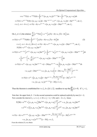
The evaluation of the integrals and skillful collection of like terms result in the following expression for Y(t) :
 
 
 
 
      
   
0 0 0
0 0 0
0
2
( ) 1 0 1 2 ( 2 )
1 0 1
3
1 0 1 3 ( 3 ) ( 2 ) 2 ( 3 )
1 1 0 1 1 1 0 1
2 2 ( 3 )
1 1 0 1
( ) ( ) 2
2!
3 2 ( 3 )
3!
3
a t a t h a t h
a t h a t h a t h
a t h
a a a
Y t e a a a t h e t h e
a a a
t h e a a a a t h e a a a a t h e
a a a a t h e
  

   
   

 

     

       
  
Observe that for {0,1,2,3} and , k k  tJ
 
      
      
    
0 0
0
0
1 0 1
1
1
1 1 0 1
1
2 2
1 1 0 1
[ 1]
( 3 )
( ) sgn max 0,
!
( [ 1] ) sgn max 0, 1
( 3 ) sgn max 0, 2 (4)
i
k
a t i
i
k
i
i
a t ih
a t i h
a t h
a a a
Y t e t ih e k
i
a a a a t i h e k
a a a a t h e k



 

 

 

  
    
 
 
    
   


A definite pattern is yet to emerge; so the process continues.
4 4 3 4 3 Now consider the interval J ; s, t  J  4h J  J ={4h} and s  h J ; hence

5. On Optimal Computational Algorithm…
www.ijmsi.org 40 | P a g e
 
       
 
0
0
3
1 0 1
1 0 1
1
2
1 0 1
0 0
0
2
4
( 4 ) 1
1
2
1
4 [3 ]
the relation (3) implies that
4 3
( ) !
i
i
i
a h i
a t h
i
h
a i h a i h
a
a a a
i h a a a i h
i
a a a
e e a e
Y t e
a h e




 
 


  
  

 
   
  
    
 
   
     
     
0 4
0 4
4 4
0 4
0 0
3
1 0 1
4
( ) 1
1 4
4 2 2 2
1 1 0 1 4 1 1 0 1 4
1
1
[ 2] ( 4 )
1
!
( [ 2] ) ( 4 )
i
a s h i
t
a t s i
h
i
i
a s i h
a s i h a s h
a a a
e s i h e
i
a e ds
a a a a s i h e a a a a s h e
   
 
   

 
  
    
      
        
       
 



   
     
     
0 4
0 4
4 4
0 4
0 0
3
1 0 1
4
( ) 1
1 4
4 4 2 2 2
1 1 0 1 4 1 1 0 1 4
1
1
[ 2] ( 4 )
1
!
( [ 2] ) ( 4 )
i
a s h i
t
a t s i
h
i
i
a s i h
a s i h a s h
a a a
e s i h e
d i
a e ds
ds
a a a a s i h e a a a a s h e
   
 

   

 
  
    
      
        
       
 



 
       
 
0
3
1 0 1
1 0 1
1
2
1 0 1
0 0
0
2
( )
1
1
2 ( 3 )
1
[ 1]
4 3
!
( )
i
i
i
a t t ih i
i
t h
a a t i h
a
a a a
i h a a a i h
i
a a a
Y t e e a e
a h e









  
  

   

 
 
 
     
 
     
 
 
 
0 0
0
0
0
3
( ) 1 1 0 1 1
1
1
3 2 2
1 1 0 1 1
1 1 1 0 1
1 1
2 2
1 1 1 0 1 1 1 1
1
1
[ 2]
1
2
4 1
( 1)!
( [ 2] )
[3 ]
( 1)! 2
([2 ] )
2
i
a t h i
i
i
i i
i i
i
i
a t i h
a t i h
a t i h
a t i h
a a a a
a t h e t i h e
i
a a a a t i h e
i h e a a a a a
i
i h e
a a a a a a a a
    

   
 
 
 
   

 
 
 
 

    

  
   


  

 
   0
3
2
0 1
( 4 ) ( 4 )
3
t h a t h
a a e  

 
 
       
     0 0 0
3 3
( ) 1 1 0 1 1 1 0 1
1 0
1 1
1 1
4 1 3
! !
i i
a t h i i
i i
a a a a a t i h a a a a a t i h
a a t h e t i h e i h e
i i
        

 
     
      
 
 
       
 
   0 0  
3 3
1 0 1 1 1 0 1 1
1 0 1 0
1 1
1 1
1 3
1 ! 1 !
i i
i i
i i
a a a a t i h a a a a t i h
a a t i h e a a i h e
i i
       
 
 
     
    
   
     
     
 
        
 
 
0 0
0 0
0
2
2 2
1 1
1 1 0 1 1 0 1 0 1
1 1
2
2
1 2 2 2
1 0 1 0 1 1 1 0 1
1
3
2 2
1 0 1 0 1
[ 2] [ 2]
[ 2] ( 4 )
( 4 )
2
( 4 )
2
2
4
2
4
3
i i
i i
i
i
a t i h a t i h
a t i h a t h
a t h
t i h
a a a a t h e a a a a a e
i h
a a a a a e a a a a t h e
t h
a a a a a e
 
   
 

   

 
   
  

 
    

    

 
 

It is evident from change of variables and grouping techniques that

6. On Optimal Computational Algorithm…
www.ijmsi.org 41 | P a g e
 
       
 
     
   
 
  
 
 
0
0 0
3
1 0 1
1
0 0
0
0
3 3
1 1 0 1 1 1 0 1 1
1 0
1 1
( ) ( ) ( )
1 1 0
3
1 1 0 1 1
1
1 1
[ 1
4
!
1 1
( 1)! 1 !
4 4
[3 ]
( 1)!
i
i
i
i i
a t i i
i i
a t h a t h t ih
i
i
i
a t i h a t i h
a
a t i
a a a
i h
i
a a a a a a a
e t i h e a a t i h e
i i
a t h e a a t h e e
a a a a
i h e
i


       

 
  

 

   
 


 
     
 
    

 


 
    
 
      
 
    0
0
0
3
1 0 1 1 1
1 0
1
4
1 0 1
1
]
3
1 !
; (5)
!
i
i t i
i
i
a t i
i
h a h
a t ih
a a a
a a i h e
i
a a a
e t ih e
i
   






 


  


 
 
 
     
 
     
   
 
 
0
0
0 0
0
2
2 2 2
1
1 1 1 0 1 1 0 1 0 1
1 1
2 2
2 2 2
1 1 0 1 1 1 0 1
2 2
2
1 1 0 1
1
[ 2]
[ 2]
3 4
[ 2]
( [ 2] ) 2
2 2
3 4
(6)
2 2
( [ 2] )
;
2
i i
i i
i
i
a t i h
a t i h
a t h a t h
a t i h
t i h e t i h
a a a a a a a a a a e
t h t h
a a a a e a a a a e
t i h e
a a a a

   
 
   
 

 
 
 
 
   
  
 
   
 
 
 

   
 
 
      
2
1 0 1
2
2
1 0 1
0
0
0 0
2 2
2 ( 3 )
1 1 1 1 0 1
1
2
2
1 ( 3 )
1 0 1 0 1 1
1
2
[ 2]
Also,
2
([2 ] )
2
2
(7)
2
t h i
i
i t h
i
a t i h
a
a t i h a
a a a
h
a a a
i h e
a h e a a a a a
i h
a a a a a e a e


 

  

 
  

 
 



 

  


      
       
 
   
   
1 0 1
0 0
0 0
0
2 3
2
1 1 1 1 0 1
1
2
1 2 2 2
1 1 0 1 1 1 0 1
1
3
3
2 2 1 1 0 1
1 0 1 0 1
1
[ 1] ( 4 )
[ 2] ( 4 )
( 4 )
Furthermore,
3
( 4 )
3
( 4 ) 4
4
1
3 !
i
i
i
i
i
i
i
a t i h a t h
a t i h a t h
a t h
a a a i h
t h
a e a a a a a e
a a a a t h e a a a a t h e
t h a a a a
a a a a a e t i h e
i
   


   

 
 

  
  

 

 
     
 
    


  
 
    
           
     
 
1 0 1
0
0
0 0
0 0
0
3
1 1 0 1
1
4 1
2 2
1 1 1 0 1
1
3
2 2 2 3
1 1 0 1 1 1 0 1
2
2
1` 1 0 1
1
1
[ 1] ( 3 )
( 4 ) ( 4 )
( 3 )
3
!
1
1 3
2
( 4 )
4
2
2
i
i
i
i
i
a t i h
a t i h
a t i h a t h
a t h a t h
a t h
a a a
a a a a
i h e
i
a t i h e a a a a t h e
t h
a a a a t h e a a a a e
h
a a a a e

 
   


  

   
 
 
 
  
 



 
     

    
 


(8)

7. On Optimal Computational Algorithm…
www.ijmsi.org 42 | P a g e
Adding up expressions (5), (6), (7) and (8) yields
 
   
     
   
0 0
0 0
0
4
1 0 1
1
4 1
2 2
1 1 0 1 1 1 0 1
1
3
3 2 2 2
1 1 0 1 1 1 0 1
[ 1] ( 3 )
( 4 )
( )
!
( [ 1] ) ( 3 )
( 4 ) 3
( 4 ) (9)
2 2
i
a t i
i
i
i
a t ih
a t i h a t h
a t h
a a a
Y t e t ih e
i
a a a a t i h e a a a a t h e
t h
a a a a a a a a t h e



   

   

  

  
    
 
 
      
  
      
 


Hence for , 0, 1, 2, 3, 4, k tJ k
 
      
      
    
   
0 0
0
0
0
1 0 1
1
1
1 1 0 1
1
2 2
1 1 0 1
3
3 2 2 2
1 1 0 1 1 1 0 1
[ 1]
( 3 )
( ) sgn max 0,
!
( [ 1] ) sgn max 0, 1
( 3 ) sgn max 0, 2
( 4 ) 3
( 4 )
2 2
i
k
a t i
i
k
i
i
a t ih
a t i h
a t h
a
a a a
Y t e t ih e k
i
a a a a t i h e k
a a a a t h e k
t h
a a a a a a a a t h e



 

 
   

 

  
    
 
 
    
   
  
      
 


   ( 4 ) sgn max 0, 3 (10) t h k  
   
 
 
0 1
1
1
Observe that for , , 1,2, , ; and 1, 1,2, , 1 . The transformation
!
from ( ) to ( ) requires only the computations of , for 1,2, , 1 2 ,
2,3, , 1 , 3, such that 1, sin
k j i
k k i j
t J c j k c i k
j
Y t Y t c i k
j k i k i j k

     
  
      
 

 1
1 2 1 3 2 1 2
ce is already known for each . Therefore
one need only determine 1 new values, namely , , , , .
i
i j k k k k
c i
k c c c c c     
On a positive note, the author has successfully devised an optimal computational algorithm for the
solution matrices without recourse to the class of differential equations (1) and expression (3), usi
1( ) as a starting point. This is the focus of the next res t.
ng
Y t ul
1 1  3. Main Result: A computational Algorithm for transiting from ( ) to ( ),  k k Y t Y t k
    1 2 1 1 0 1 Let , let , 0,1 . Suppose that 0. k t J a a a a        
 
 
   
      
 
2
1 2
1 2
2
1 2
1 2
2
1
0
0
1 0 1
1 1 1
1 1 2
1
1
1 0 1 1
1
1 1 2
1 0 1
1
2 2
[ 1]
[ 2]
( ) ( ) ( ) [ 1]
!
( [ 1] ) sgn max 0, 1
1
( [
1 ( 1)sgn( )
j
k
j
k
j
k
i
i
j
i
i j
a t j h
a t i h
a a a
Y t Y t Y t a t j h e
j
a a a
a t i h e k
a a a
c a t i j
j

 
 

 
 




 

 
 
  


  

  

 

 
 

    


   


   
  
 
 
     2
1 2
0
2
1 1 2
[ 1]
1] ) sgn max 0, 2 (11)
for some real positive constants secured from ( ),with the process initiated at 1.
k k i
j
i j
i j k
a t i j h
h e k
c Y t k

 
 

   
  


 
3.1 Remarks on the optimal computational algorithm

8. On Optimal Computational Algorithm…
www.ijmsi.org 43 | P a g e
      
2
1 2
1 2
0
1
1 1
1
1 0 1
1
1 0 1 2
[ 1]
Observe that for , ( ) can be expressed in the equivalent form
( ) ( )
( [ 1] ) sgn max 0, 1 (12)
1 sgn( )
for some real posit
k k
k
j
k k i
i j
i j
i j
a t i j h
t J Y t
Y t Y t
a a a
c a t i j h e k
j

 
  



 
  

   
  



    
  
   
0 1
ive constants secured from ( ),with the process initiated at 1.
1
Moreover , 1,2, , 1 ; 1, 1,2, , and the transformation from ( )
!
i j k
j i k
c Y t k
c j k c i k Y t
j

      
    1
1 2 1 3 2 1 2
to ( ) requires only the computations of for 1,2, , 1 2 , 2,3, , 1 ,
3, such that 1.Therefore one need only determine 1 new values, namely
, , , , .

  
     
     
 

k i j
i j
k k k k
Y t c i k j k i
k i j k k c
c c c c
3.2 Interpretation of the computational algorithm for Y(t)
  1 1 Stage 1:Transiting from ( ) to ( ), 1, 2, 3, k k Y t Y Y t k    
 0  Perform the following operations on each term of ( ) : a t
k Y t e
 
      1 0 1  1 0 1  0   0  
-1 1 0 1
power of power of [.] [.]
Increment each power of by 1; preserve the power of
Let
(i) a
(ii) [.] [.] ;
a a a a a a a t h a t h h
a a a
t h t h h e e  

    

    
     0  The operations i and ii yield exactly the same number of terms as in ( ) a t
k Y t e
 
           
1 0 1 1
1 0 1 1 0 1 0 0 exponent of 1+ old exponent of [.] [.]
(iii) Increment each exponent of by 1; preserve the exponent of
(iv) Let [.] [.] ;
(v) Divide each term by the new e
a a a a a a a t h a t h h
a a a a
t h t h h e e
 
      

    
 
   
   
1 0 1
1 0 1 1 0 1
1 0 1 1 0 1
xponent of resulting from operation (iii),
where new exponent of 1 old (preceding) exponent of , that is
new exponent of exponent of from the resulting term in
a a a
a a a a a a
a a a a a a

 
 

   
  
 
1
1 0 1
( )
1 exponent of from the term operated on, in ( )
k
k
Y t
a a a Y t


  
      0 The operations iii , (iv) and v yield exactly the same number of terms as in ( ) a t
k Y t  e
   1 1 0 1
(vi) Aggregate all terms resulting from operations (i) to (v) through appropriate groupings
of common factors of powers of a and a a a .
 

    1 1 1 Stage 2: Transiting from ( ) to ( ), 1,2, 3, k k Y Y t Y t k     
 0   
1 1
1 1
Secure by adding to the aggregated terms in (vi); in order words
the resultant expressions from the application of the algorithm to
( ) ( )
1, 2,3,
( ) ( )
( ) ;
k
k a t
k
Y t Y t
Y k
Y t Y t
t e

 
 
  
  
 

3.3 Cardinality and CardinalityTransition Analyses on ( ) k Y t
    1 Denote the cardinality of . by . . Then ( ) ( ) 1 is the resulting autonomous     k k Y t Y t k
nonhomogeneous linear difference equation, for k1, 2, 3,. Hence
  
  1 1
1 2
( ) 1 , 0, 2, 3, ,noting that ( ) 2.
2 
 
     k
k k
Y t k Y t

9. On Optimal Computational Algorithm…
www.ijmsi.org 44 | P a g e
   
     
 
0
0
1 1
Furthermore, for 1,2, , the number of terms that need to be aggregated from ( )
to secure ( ) ( ) is 1 ,derived from the fact that there are 2 ( )
2 ( ) 1 such terms. Therefore

 
  
 
 a t
k
a t
k k
k
k Y t e
Y t Y t k k Y t e
Y t k2
1
2 terms must be aggregated in the transition from
( ) to ( ). 
 
k k
k
Y t Y t
3.4 Verification and illustrations of Algorithm 3
0
0
0 0 0
0
1 1 ([ ] )
([ ] ) 1 0 1
2 2 1 1 1 0 1
( ) ([ ] )
2 1 0 1 1 1 0 1
1 1 1 1 ([ ] )
1 0 1
( ) ([ ] )
( ) ( ) ( )([ ] )
1 1
( ) ( )( ) ( )([ ] )
( ) ([ ] )
1 1
a t h h
a t h h
a t a t h a t h h
a t h h
a a a t h h e
t J Y t Y t a a a a t h h e
Y t e a a a t h e a a a a t h h e
a a a t h h e
  
  
 
  
  
   

  
       

       
  


    
0
0 0
2 1 1 ([ ] )
1 0 1 2
1 1 0 1 2
1
( ) ( )
( ) ( 2 ) , .
!
i a t h h
a t a t h
i
a a a t ih e
Y t e a a a a t h e t J
i
  
 
 

 
     
  3 4
It is straight-forward and easy to check that the algorithm verifies the rest of the computation
( ), for 3 ,5
s for
.
Y t tJ J  h h
  5 Finally, we apply the algorithm to extend the solution matrices to the interval J  5h,6h .
    1 4 23 32
4 5
To achieve this, set 4, so that 1 5; so we need only obtain the 1 4 1 3
new coefficients , for 1,2,3 , 2, ,5 : 1, namely , and .
The application of the algorithm from to yie
i j
k k k
c i j i i j k c c c
J J
      
      
5 lds the following expression for Y(t), tJ :
 
   
     
   
 
0
0 0
0
4
1 0 1
1 1
1
4 1
1 2 2 2
1 1 0 1 1 1 0 1
1
3
2 3 3 2 2
1 1 0 1 1 1 0 1
1 0 1
[ 1]
[ 1] ( 4 )
( 5 )
( ) ( ) [ 1]
!
( [ 1] ) ( 4 )
( 5 ) 3
( 5 )
2 2





   

   

 
  

  
     
 
 
      
  
      
 




j
j
j
i
i
a t j h
a t i h a t h
a t h
a a a
Y t Y t a t j h e
j
a a a a t i h e a a a a t h e
t h
a a a a a a a a t h e
a a a
 
   
     
   
0
0 0
0
1
4
1
2 3
4 1
1 0 1 1 0 1 2
1 1
1
4
4 2 3 2
1 1 0 1 1 1 0 1
[ 1]
[ 1] ( 4 )
( 5 )
[ 1]
1 !
( [ 2] ) ( 4 )
2 3
( 4 ) 3
( 5 )
2(4) 2(3)



 
 

   
 
  

 
   
  
 
 
    
  
      
 


j
j
j
i
i
a t j h
a t i h a t h
a t h
t j h e
j j
a a a a a a
a t i h e a t h e
t h
a a a a a a a a t h e
1 0 5 4 1
1
Aggregation of like terms: ( ) the terms with 1 4, together with , 1,
5!
evaluate to
Y t   i  j  c  c 

10. On Optimal Computational Algorithm…
www.ijmsi.org 45 | P a g e
 
       
     
0 0 0
0 0
5 5 1
1 0 1
1 1 0 1
1 1
3
2 2 3 2 2 2
1 1 0 1 1 1 0 1 1 1 0 1
[ 1]
( 3 ) ( 4 )
( [ 1] )
!
( 4 ) 3
( 3 ) ( 4 )
2 2


 
 
     
  
 
  
       
 
 
  
         
 
 
j
a t j i
j i
a t jh a t i h
a t h a t h
a a a
e t jh e a a a a t i h e
j
t h
a a a a t h e a a a a a a a a t h e
14 23
23 1 4 2 3 32
It follows from the aggregated terms that the values of the remaining three coefficients , and
1 1 1 1 3 1 1
are , and respectively. Therefore , 1 and 2. Hence
4! 8 2 2 2 2 6
c c
c    c  c  c 
 
       
     
 
0 0 0
0 0
5 5 1
1 0 1
1 1 0 1
1 1
3
2 2 3 2 2 2
1 1 0 1 1 1 0 1 1 1 0 1
4
4
1 1 0 1
[ 1]
( 3 ) ( 4 )
( ) ( [ 1] )
!
( 4 ) 3
( 3 ) ( 4 )
2 2
( 4 )
3!


 
 
     
  
  
 
  
        
 
 
  
         
 

  
 
j
a t j i
j i
a t jh a t i h
a t h a t h
a a a
Y t e t jh e a a a a t i h e
j
t h
a a a a t h e a a a a a a a a t h e
t h
a a a a a     0
2 3 3 3 2 2
1 1 0 1 1 1 0 1 5
( 5 ) ( 5 ) 2 ( 5 ) ; .   
  
       
 
a t h a a a t h a a a a t h e t J
5
0
Moreover the general expresion for ( ), can be stated as follows: k
k
Y t t J


 
     
     
   
   
0 0
0
0
0
5
1 0 1
1
5 1
1 1 0 1
1
2 2
1 1 0 1
3
3 2 2 2
1 1 0 1 1 1 0 1
[ 1]
( 3 )
( 4 )
( ) max ,0
!
( [ 1] ) max 1,0
( 3 ) max 2,0
( 4 ) 3
( 4 ) max
2 2
j
a t j
j
i
i
a t jh
a t i h
a t h
a t h
a a a
Y t e t jh e k
j
a a a a t i h e k
a a a a t h e k
t h
a a a a a a a a t h e



 

 
   

 


  
    
 
 
    
   
  
      
 


 
   
 
0  
4
4 2 3 3
1 1 0 1 1 1 0 1
3 2 2
1 1 0 1
( 5 )
3,0
( 4 )
( 5 )
3! max 4,0 .
2 ( 5 )
a t h
k
t h
a a a a a a a a t h
e k
a a a a t h
   
 


  
     
   
     
IV. CONCLUSION
This article obtained an optimal computational schemefor the structure of the solution matrices of
single-delay linear neutral differential equations by leveraging on the established expressions for such matrices
on the time interval of length equal to five times the delay, starting from time zero. The scheme is iteratively
based on transitions fromone time interval of length equal to the delay to the next contiguous intervalof
length h , with the coefficients from the preceding interval preserved, two new coefficients updatedand the rest
obtained from the aggregation of the components resulting from the afore-mentioned transitions. This algorithm
alleviates the computational burden associated with relying on the equation (1) and the expression (3) fraught
with proneness to computational errors and resolves to a great extent the lack of a general expression for the
solution matrices.The structure of the algorithm is so simple that the solution matrix transitions from one
interval to the next contiguous interval can be obtained by inspection and addition of two terms for each new
coefficient.

11. On Optimal Computational Algorithm…
www.ijmsi.org 46 | P a g e
REFERENCES [1] Ukwu, C. (1987). Compactness of cores of targets for linear delay systems., J. Math. Analy.and Appl., Vol. 125, No. 2, August 1. pp. 323-330. [2] Ukwu, C. and Garba, E.J.D. (2014w).Construction of optimal expressions for transition matrices of a class of double – delay scalar differential equations. African Journal of Natural Sciences (AJNS). Vol. 16, 2014. [3] Ukwu, C. and E. J. D. Garba (2014e). Derivation of an optimal expression for solution matrices of a class of single-delay scalar differential equations. Journal of Nigerian Association of Mathematical Physics. Vol. 26, March 2014.