Download as PDF, PPTX


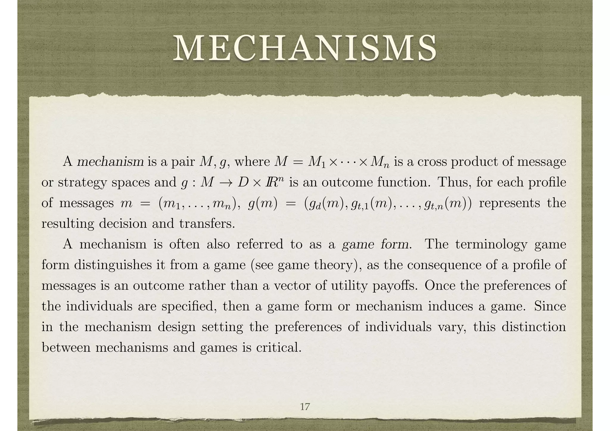


![INDIVIDUAL IRRATIONALITY
IN GROVES’ SCHEMES
if individual 1 were not present. The result will be feasible and any surplus generated
can be given to individual 1. The overall mechanism will be balanced, but the decision
will not be e cient. However, the per-capita loss in terms of e ciency will be at most
maxd,d0,✓1 [v1(d, ✓1) v1(d0
, ✓1)]/n. If utility is bounded, this tends to 0 as n becomes
large. While this obtains approximate e ciency, it still retains some di culties in
terms of individual rationality. This is discussed next.
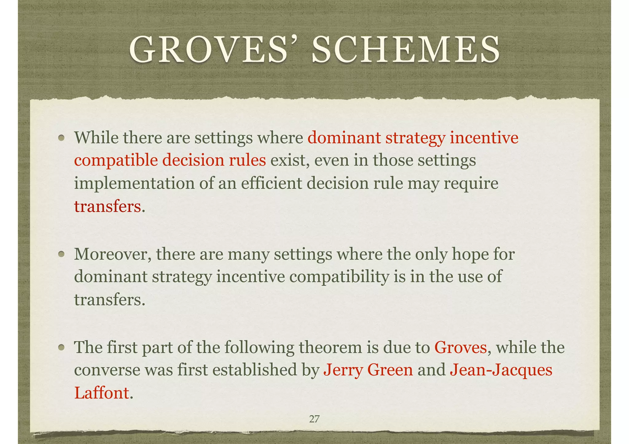
3.9 Lack of Individual Rationality in Groves’ Schemes
In addition to the balance problems that are present with trying to achieve an e cient
decision with a dominant strategy mechanism, there are related problems. One is the
violation of what is commonly referred to as an individual rationality or voluntary
participation condition.9
That requires that vi(d(✓), ✓i) + ti(✓) 0 for each i and ✓,
assuming a proper normalization of utility. As we argued above in the example above,
at least one of 1
4
t1(0, 1)+t2(0, 1) or 1
4
t1(1, 0)+t2(1, 0) holds. Since no project
is built in these cases, this implies that some individual ends up with a negative total
utility. That individual would have been better o↵ by not participating and obtaining
a 0 utility.
3.10 Ine cient Decisions
Groves’ schemes impose e cient decision making and then set potentially unbalanced
32](https://image.slidesharecdn.com/slidemcden-151107075938-lva1-app6891/75/Introduction-to-Mechanism-Design-32-2048.jpg)
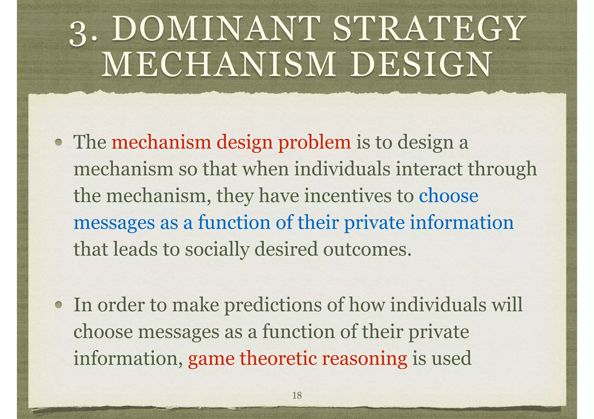
![INEFFICIENT DECISIONS
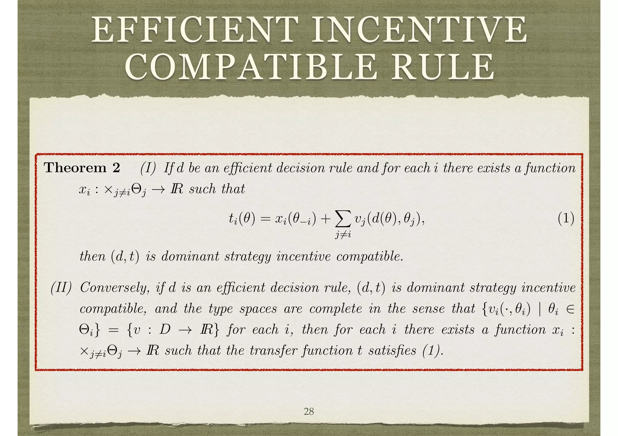
3.10 Ine cient Decisions
Groves’ schemes impose e cient decision making and then set potentially unbalanced
transfers to induce incentive compatibility. An alternative approach is to impose bal-
ance and then set decision making to induce incentive compatibility. This approach
was taken by Herv´e Moulin and strengthened by Shigehiro Serizawa in the context of
a public good decision. It results in a completely di↵erent set of social choice functions
from the Groves’ schemes, which is outlined here in a special case.
Let D = [0, 1]⇥IRn
+ where d = (y, z1, . . . , zn) is such that
P
i zi = cy, where c > 0 is
a cost per unit of production of y. The interpretation is that y is the level of public good
chosen and z1 to zn are the allocations of cost of producing y paid by the individuals.
9
Another problem is that Groves’ schemes can be open to coalitional manipulations even though
they are dominant strategy incentive compatible. For example in a pivotal mechanism individuals
may be taxed even when the project is not built. They can eliminate those taxes by jointly changing
their announcements.
17
The class of admissible preferences di↵ers from the quasi-linear case focused on above.
An individual’s preferences are represented by a utility function over (d, t, ✓i) that takes
the form wi(y, ti zi, ✓i) where wi is continuous, strictly quasi-concave, and monotonic
in its first two arguments, and all such functions are admitted as ✓i varies across ⇥i.
In the situation where no transfers are made and costs are split equally, the resulting
wi(y, cy/n, ✓i) is single-peaked over y, with a peak denoted byi(✓i).
Theorem 3 In the above described public good setting, a social choice function (d, t)
is balanced, anonymous,10
has a full range of public good levels, and dominant strategy
incentive compatible if and only if it is of the form ti(✓) = 0 for all i and d(✓) =
(y(✓), cy(✓)/n, . . . , cy(✓)/n), where there exists (p1, . . . , pn 1) 2 [0, 1]n 1
33](https://image.slidesharecdn.com/slidemcden-151107075938-lva1-app6891/75/Introduction-to-Mechanism-Design-33-2048.jpg)
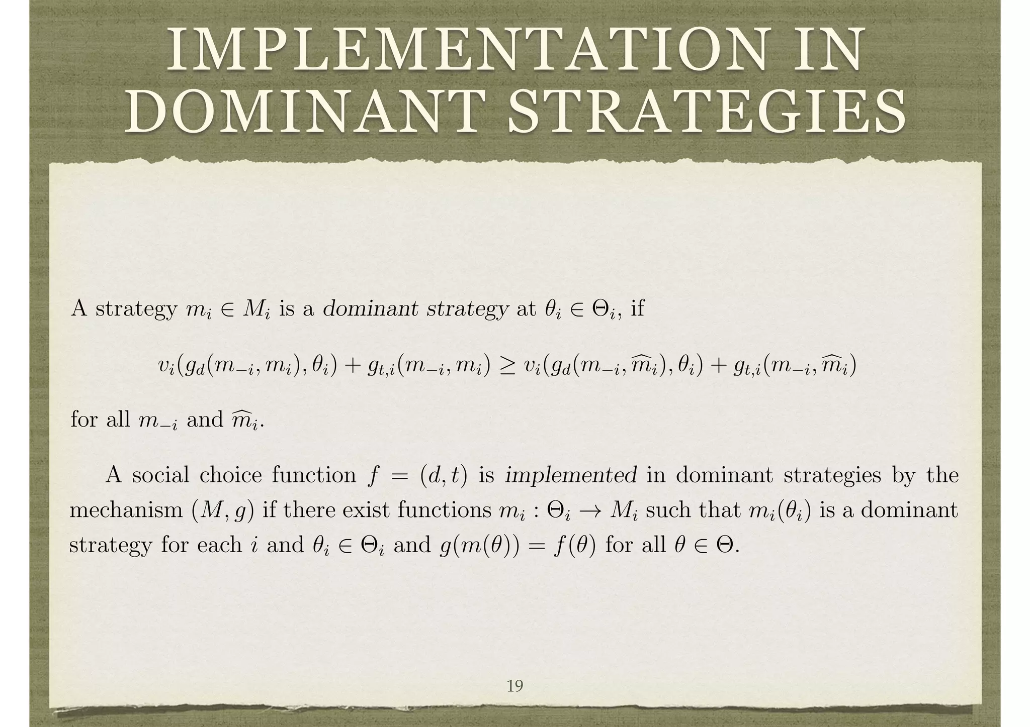
![in its first two arguments, and all such functions are admitted as ✓i varies across ⇥i.
In the situation where no transfers are made and costs are split equally, the resulting
wi(y, cy/n, ✓i) is single-peaked over y, with a peak denoted byi(✓i).
Theorem 3 In the above described public good setting, a social choice function (d, t)
is balanced, anonymous,10
has a full range of public good levels, and dominant strategy
incentive compatible if and only if it is of the form ti(✓) = 0 for all i and d(✓) =
(y(✓), cy(✓)/n, . . . , cy(✓)/n), where there exists (p1, . . . , pn 1) 2 [0, 1]n 1
y(✓) = median [p1, . . . , pn 1, by1(✓1), . . . , byn(✓n)] .
If in addition individual rationality is required, then the mechanism must be a minimum
demand mechanism( y(✓) = mini byi(✓i)).
The intuition Theorem 3 relates back to the discussion of single-peaked preferences.
The anonymity and balance conditions, together with incentive compatibility, restrict
the ti’s to be 0 and the zi’s to be an even split of the cost. Given this, the preferences of
individuals over choices y are then single-peaked. Then the phantom voting methods
described in section 3.4 govern how the choice. The expression for y(✓) fits the phantom
voting methods, where p1, . . . , pn 1 are the phantoms.
The answer to the question of which approach - that of fixing decisions to be e cient
and solving for transfers, or that of fixing transfers to be balanced and solving for
decisions - results in “better” mechanisms is ambiguous.11
There are preference profiles
34](https://image.slidesharecdn.com/slidemcden-151107075938-lva1-app6891/75/Introduction-to-Mechanism-Design-34-2048.jpg)

![INDEPENDENT TYPES
4.2 A Balanced Mechanism with Independent Types
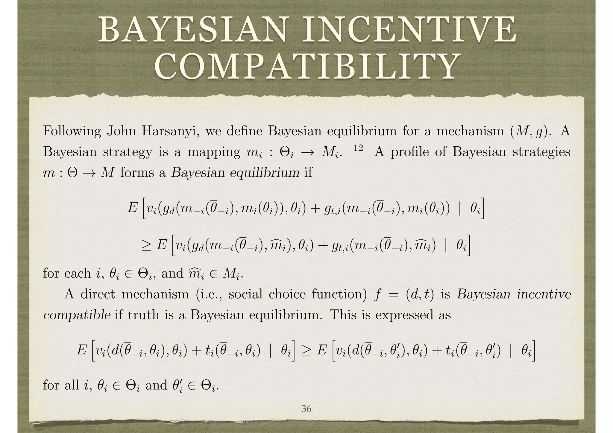
To get a feeling for the implications of the weakening of dominant strategy incentive
compatibility to that of Bayesian incentive compatibility, let us examine the case of
independent types. The mechanisms of d’Aspremont and Gerard-Varet, and of Arrow,
can then be expressed as follows.
Theorem 4 If types are independent (✓ i and ✓i are independent for each i), d is
e cient, and
ti(✓) = E
2
4
X
j6=i
vj(d(✓), ✓j) | ✓i
3
5
1
n 1
X
k6=i
E
2
4
X
j6=k
vj(d(✓), ✓j) | ✓k
3
5 ,
then (d, t) is Bayesian incentive compatible and t is balanced.
Theorem 4 has a converse just as Theorem 2 did. Here it is that if (d, t) is Bayesian
incentive compatible, d is e cient, and t is balanced, then t is of the form above plus
a function xi(✓) such that
P
i xi(✓) = 0 and E[xi(✓) | ✓i] does not depend on ✓i.13
Proof of Theorem 4: The balance of t follows directly from its definition. Let us
verify that (d, t) is Bayesian incentive compatible.
E
h
vi(d(✓ i, ✓0
i), ✓i) + ti(✓ i, ✓0
i) | ✓i
i 38](https://image.slidesharecdn.com/slidemcden-151107075938-lva1-app6891/75/Introduction-to-Mechanism-Design-38-2048.jpg)
![a function xi(✓) such that
P
i xi(✓) = 0 and E[xi(✓) | ✓i] does not depend on ✓i.13
Proof of Theorem 4: The balance of t follows directly from its definition. Let us
verify that (d, t) is Bayesian incentive compatible.
E
h
vi(d(✓ i, ✓0
i), ✓i) + ti(✓ i, ✓0
i) | ✓i
i
= E
h
vi(d(✓ i, ✓0
i), ✓i) | ✓i
i
+ E
2
4
X
j6=i
vj(d(✓), ✓j) | ✓0
i
3
5
1
n 1
X
k6=i
E
2
4E
2
4
X
j6=k
vj(d(✓), ✓j) | ✓k
3
5 | ✓i
3
5 .
13
Note that it is possible for E[xi(✓) | ✓i] not to depend on ✓i and yet xi(✓) to depend on ✓. For
instance, suppose that each ⇥k = { 1, 1} and that xi(✓) = ⇥k✓k.
20
Under independence, this expression becomes
= E
2
4vi(d(✓ i, ✓0
i), ✓i) +
X
j6=i
vj(d(✓ i, ✓0
i), ✓j) | ✓i
3
5
1
n 1
X
k6=i
E
2
4
X
j6=k
vj(d(✓), ✓j)
3
5 .
The second expression is independent of the announced ✓0
i, and so maximizing
E
h
vi(d(✓ i, ✓0
i), ✓i) + ti(✓ i, ✓0
i) | ✓i
i
with respect to ✓0
i boils down to maximizing:
E
2
4vi(d(✓ i, ✓0
i), ✓i) +
X
j6=i
vj(d(✓ i, ✓0
i), ✓j) | ✓i
3
5 .
Since d is e cient, this expression is maximized when ✓0
i = ✓i.
Note that truth remains a best response even after ✓ i is known to i. Thus, the
39](https://image.slidesharecdn.com/slidemcden-151107075938-lva1-app6891/75/Introduction-to-Mechanism-Design-39-2048.jpg)
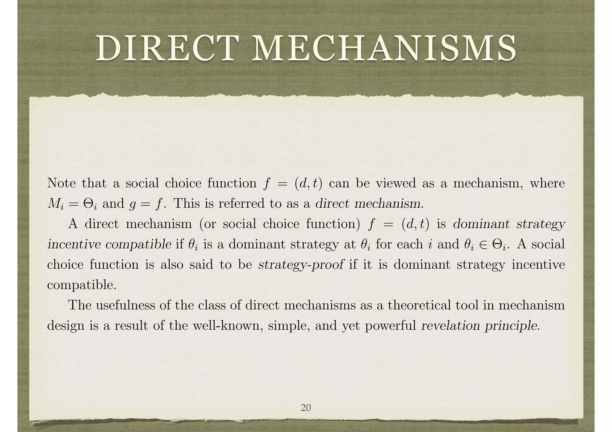
![DEPENDENT TYPES
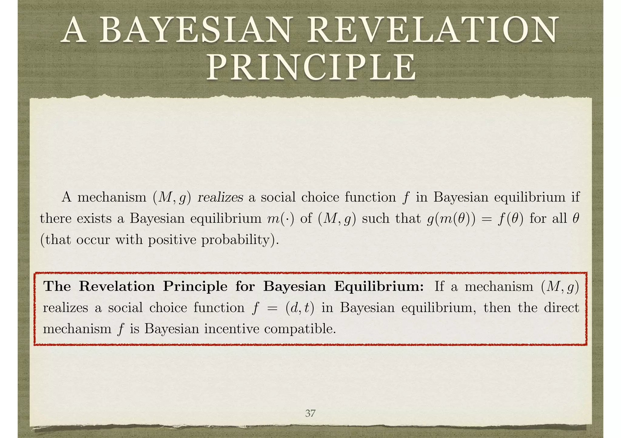
The independence condition in Theorem 4 is important in
providing the simple structure of the transfer functions, and
is critical to the proof.
Without independence, it is still possible to find an efficient,
balanced, Bayesian incentive compatible mechanisms in
“most” settings.
Since d is e cient, this expression is maximized when ✓0
i = ✓i.
Note that truth remains a best response even after ✓ i is known to i. Thus, the
incentive compatibility is robust to any leakage or sharing of information among the
individuals. Nevertheless, the design of the Bayesian mechanisms outlined in Theo-
rem 4 still requires knowledge of E[· | ✓i]’s, and so such mechanisms are sensitive to
particular ways on the distribution of uncertainty in the society.
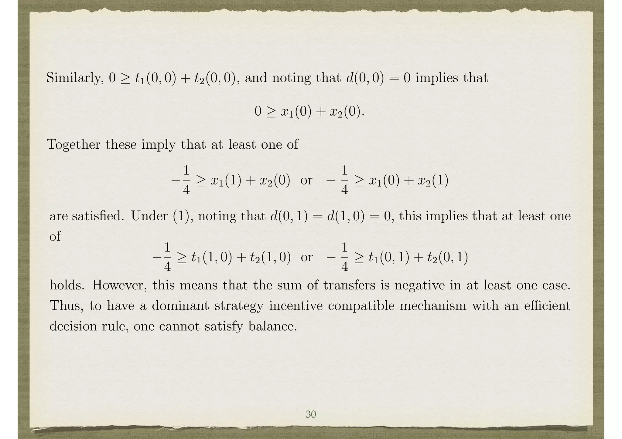
4.3 Dependent Types
The independence condition in Theorem 4 is important in providing the simple struc-
ture of the transfer functions, and is critical to the proof. Without independence, it is
still possible to find e cient, balanced, Bayesian incentive compatible mechanisms in
“most” settings. The extent of “most” has been made precise by d’Aspremont, Cr´emer,
and Gerard-Varet by showing that “most” means except those where the distribution
of types is degenerate in that the matrix of conditional probabilities does not have full
rank, which leads to the following theorem.
Theorem 5 Fix the finite type space ⇥ and the decisions D. If n 3, then the set of
probability distributions P for which there exists a Bayesian incentive compatible social
choice function that has an e cient decision rule and balanced transfers, is an open
and dense subset of the set of all probability distributions on ⇥.14
To get a feeling for how correlation can be used in structuring transfers, see Example
40](https://image.slidesharecdn.com/slidemcden-151107075938-lva1-app6891/75/Introduction-to-Mechanism-Design-40-2048.jpg)
![INTERIM IR
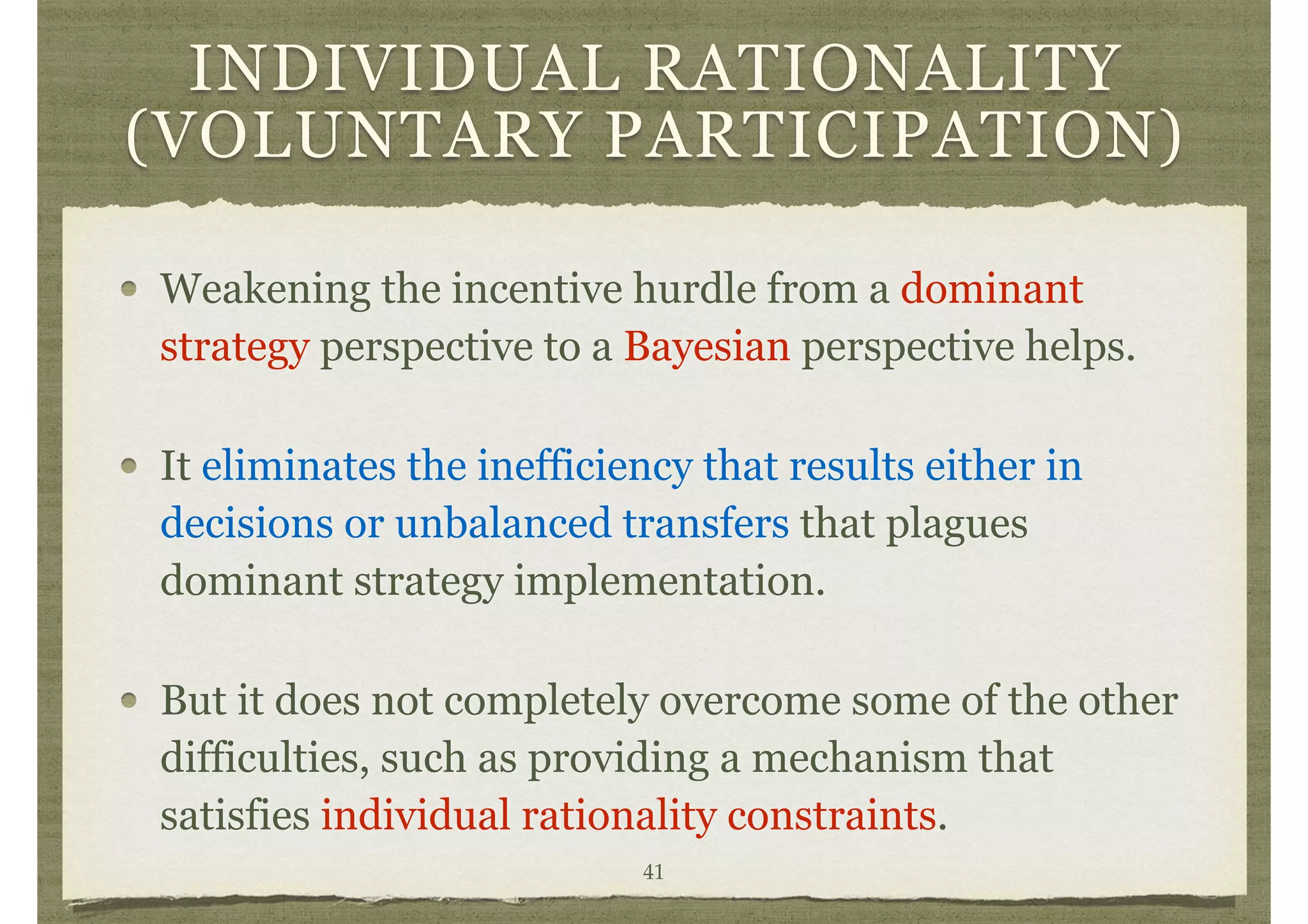
individual i would get from not participating in the mechanism for any ✓i.
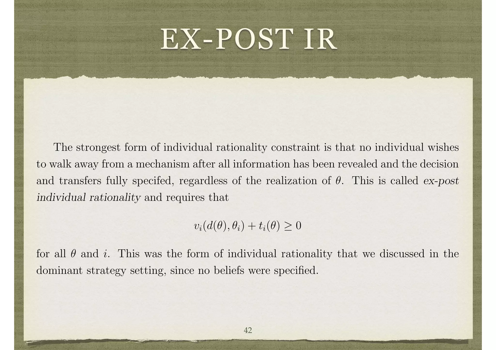
The strongest form of individual rationality constraint is that no individual wishes
to walk away from a mechanism after all information has been revealed and the decision
and transfers fully specifed, regardless of the realization of ✓. This is called ex-post
individual rationality and requires that
vi(d(✓), ✓i) + ti(✓) 0
for all ✓ and i. This was the form of individual rationality that we discussed in the
dominant strategy setting, since no beliefs were specified.
A weaker form of individual rationality is that no individual wishes to walk away
from the mechanism at a point where they know their own type ✓i, but only have
expectations over the other individuals’ types and the resulting decision and transfers.
This is called interim individual rationality and requires that
E
h
vi(d(✓), ✓i) + ti(✓) | ✓i
i
0
for all i and ✓i 2 ⇥i.
15
The time perspective can give rise to di↵erent versions of e ciency as well. However, in terms
of maximizing
P
i vi the time perspective is irrelevant as maximizing E[
P
i vi(d(✓), ✓i)] is equivalent
to maximizing
P
i vi(d(✓), ✓i) at each ✓ (given the finite type space). If one instead considers Pareto
e ciency, then the ex-ante, interim, and ex-post perspectives are no longer equivalent.
43](https://image.slidesharecdn.com/slidemcden-151107075938-lva1-app6891/75/Introduction-to-Mechanism-Design-43-2048.jpg)
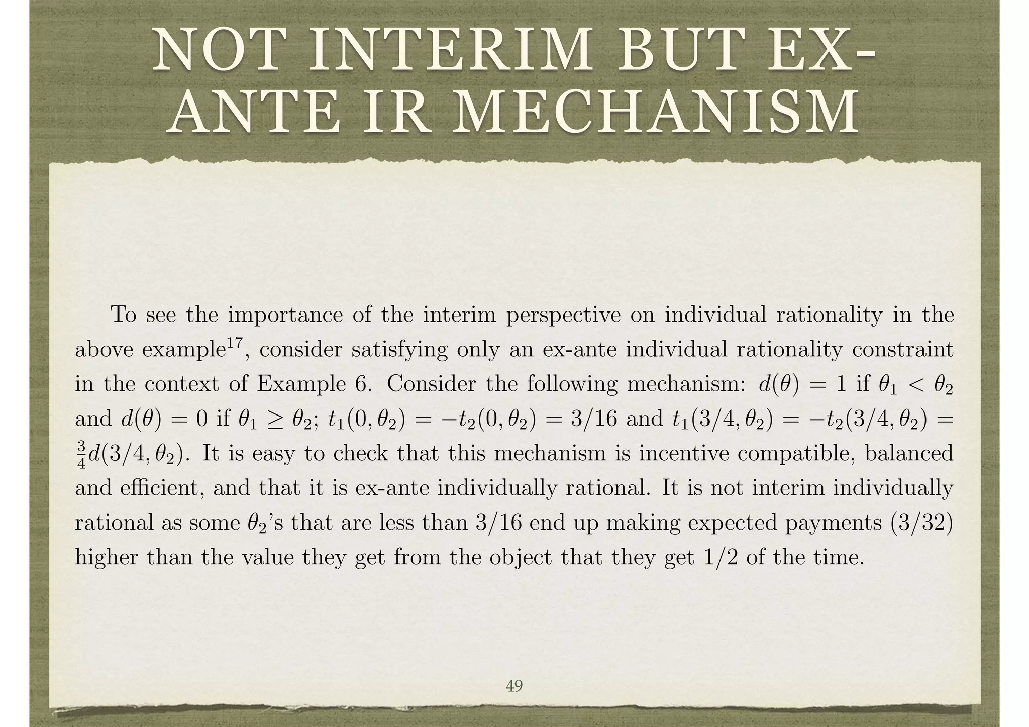
![EX-ANTE IR
The weakest form of individual rationality is that no individual wishes to walk away
from the mechanism before they know their own type ✓i, and only have expectations
over all the realizations of types and the resulting decision and transfers. This is called
ex-ante individual rationality and requires that
E
h
vi(d(✓), ✓i) + ti(✓)
i
0
for all i.
Consider any social choice function (d, t) such that
P
i E[vi(d(✓), ✓i) + ti(✓)] 0.
This will generally be satisfied, as otherwise it would be better not to run the mecha-
nism at all. Then if (d, t) does not satisfy ex-ante individual rationality, it is easy to
alter transfers (simply adding or subtracting a constant to each individual’s transfer44](https://image.slidesharecdn.com/slidemcden-151107075938-lva1-app6891/75/Introduction-to-Mechanism-Design-44-2048.jpg)
![LACK OF IR IN
BARGAINING
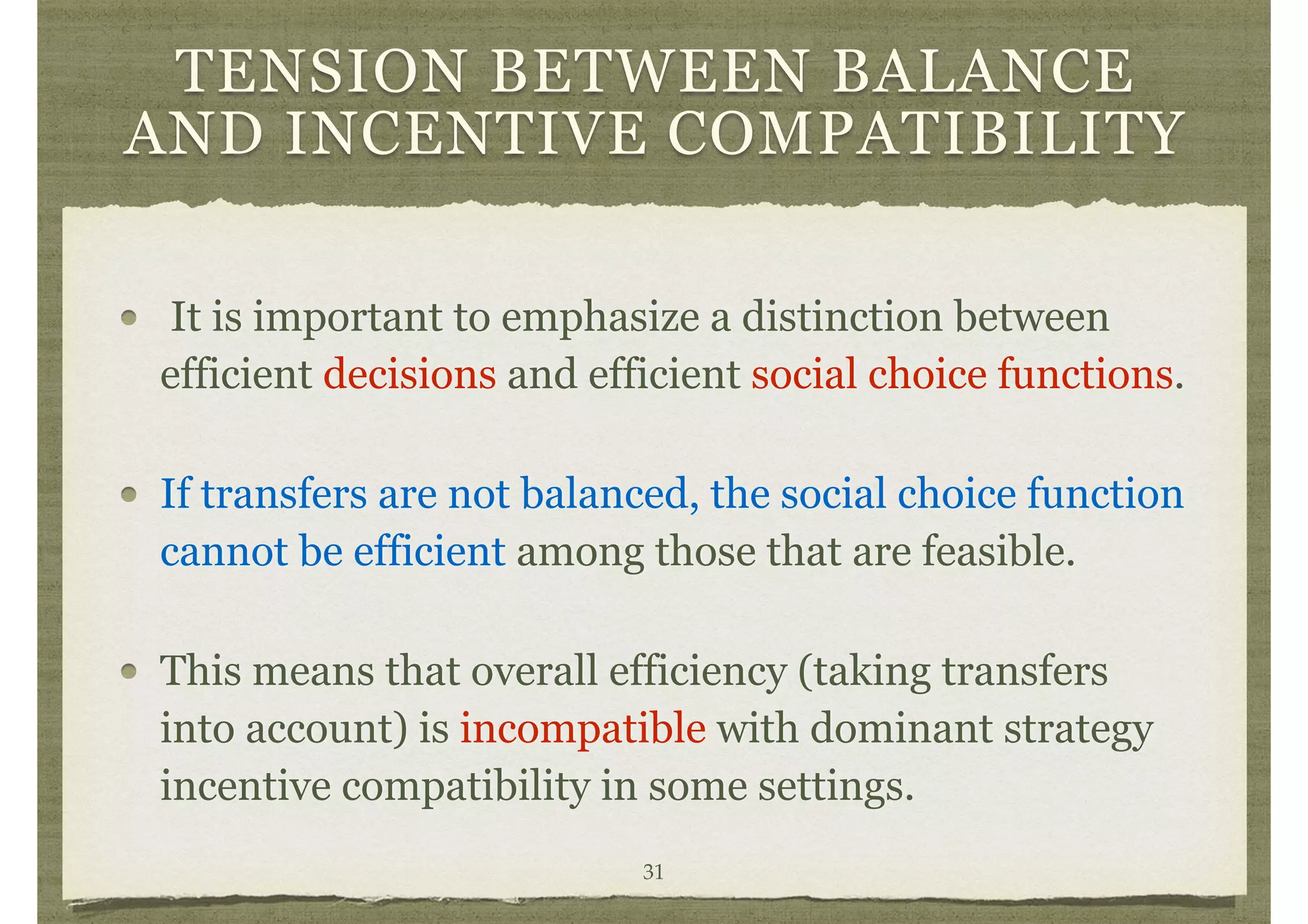
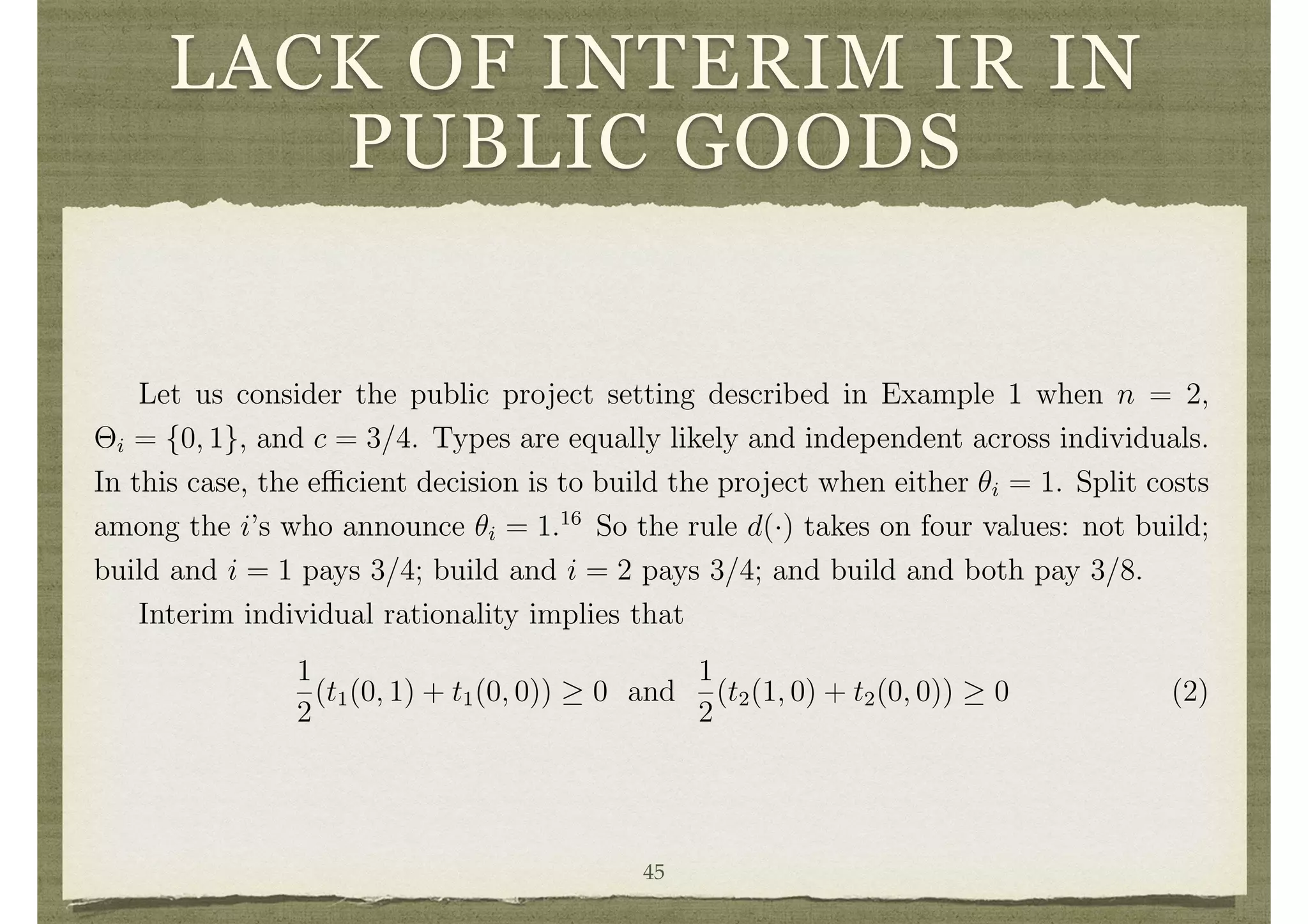
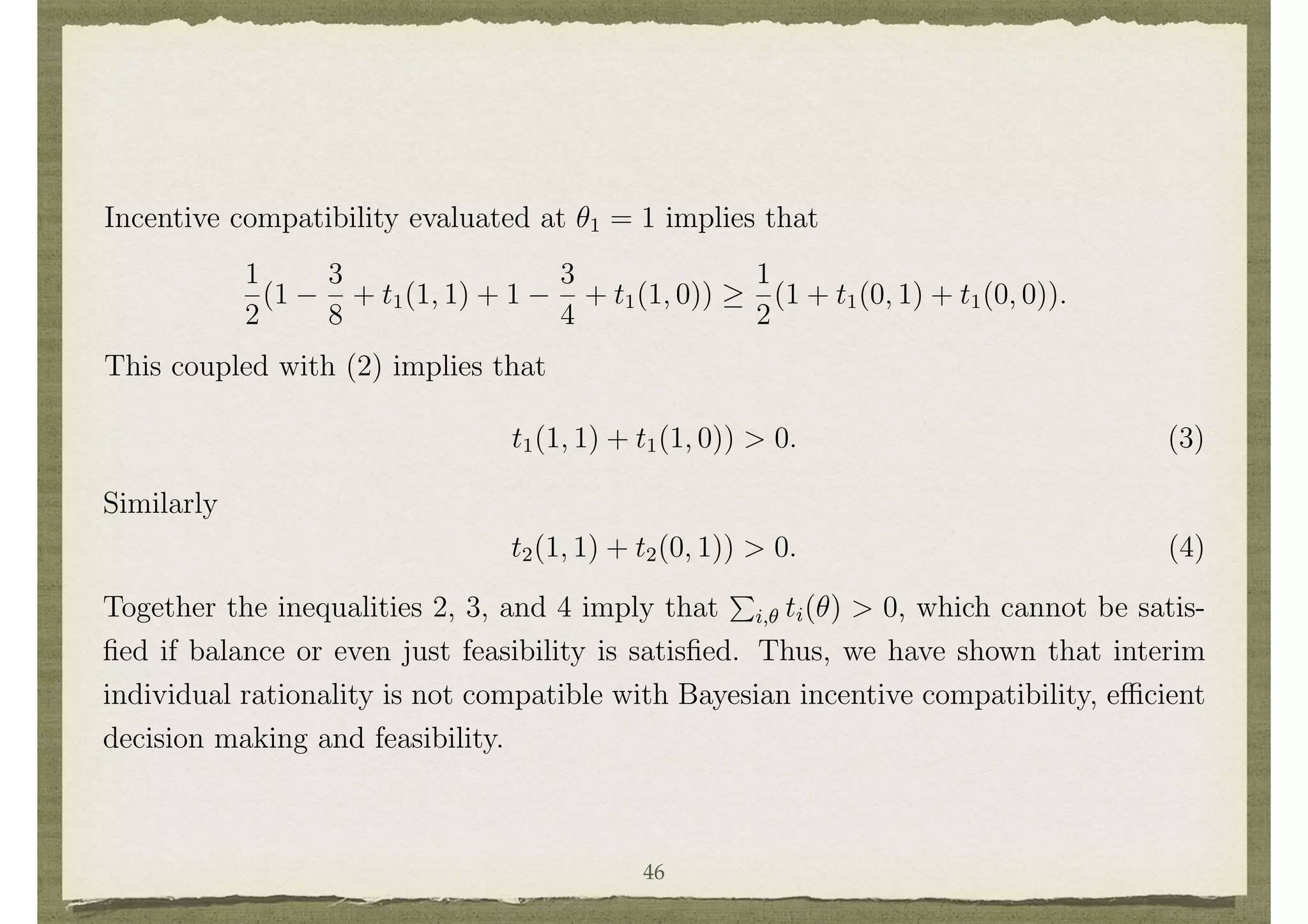
decision making and feasibility.
Finding mechanisms that take e cient decisions, are incentive compatible, balanced
and interim individually rational, is not simply a problem in public goods settings, but
is also a problem in private goods settings as was pointed out by Roger Myerson and
Mark Satterthwaite. That point is illustrated here in the context of a simple example.
Example 6 Lack of Interim Individual Rationality in a Bargaining Setting
A seller (i = 1) has an indivisible object worth ✓1 which takes on values in ⇥1 =
{0, 3/4} with equal probability. A buyer has a value for the object of of ✓2 that takes on
values in ⇥2 = [0, 1] according to a uniform distribution. A decision is a specification
in D = {0, 1} where 0 indicates that the object stays in the seller’s hands, while 1
indicates that the object is traded to the buyer.
An e cient decision is d(✓) = 1 if ✓2 > ✓1, and d(✓) = 0 if ✓2 < ✓1. Interim
individual rationality requires that if ✓2 < 3/4 (noting that these types only trade 1/2
of the time), then 1
2
✓2 + E[t2(✓1, ✓2)] 0, or
E[t2(✓1, ✓2)]
1
2
✓2. (5)
Since an e cient decision is the same for any 0 < ✓2 < 3/4 and 0 < ✓0
2 < 3/4, Bayesian
incentive compatibility implies that t2(✓1, ✓2) is constant across 0 < ✓2 < 3/4. Then
(5) implies that for any 0 < ✓2 < 3/4
47](https://image.slidesharecdn.com/slidemcden-151107075938-lva1-app6891/75/Introduction-to-Mechanism-Design-47-2048.jpg)
![E[t2(✓1, ✓2)]
1
2
✓2. (5)
Since an e cient decision is the same for any 0 < ✓2 < 3/4 and 0 < ✓0
2 < 3/4, Bayesian
incentive compatibility implies that t2(✓1, ✓2) is constant across 0 < ✓2 < 3/4. Then
(5) implies that for any 0 < ✓2 < 3/4
E[t2(✓1, ✓2)] 0. (6)
Interim individual rationality for sellers of type ✓1 = 3/4 (who expect to trade 1/4 of
the time) implies that (3
4
)2
+E[t1(3/4, ✓2)] 3
4
or E[t1(3/4, ✓2)] 3/16. Then incentive
compatibility for type ✓1 = 0 implies that E[t1(0, ✓2)] 3/16. Thus, E[t1(✓)] 3/16.
Feasibility then implies that 3/16 E[t2(✓)]. Then by (6) it follows that
3
4
E[t2(✓1, ✓2)]
24
for some ✓2 3/4. However, this, 1 ✓2 > 3/4, and (6) then imply that
✓2
2
+ E[t2(✓1, 0)] ✓2 + E[t2(✓1, ✓2)],
which violates incentive compatibility.
Thus, there does not exist a mechanism that satisfies interim individual rationality,
feasibility, e ciency, and Bayesian incentive compatibility in this setting.
48](https://image.slidesharecdn.com/slidemcden-151107075938-lva1-app6891/75/Introduction-to-Mechanism-Design-48-2048.jpg)


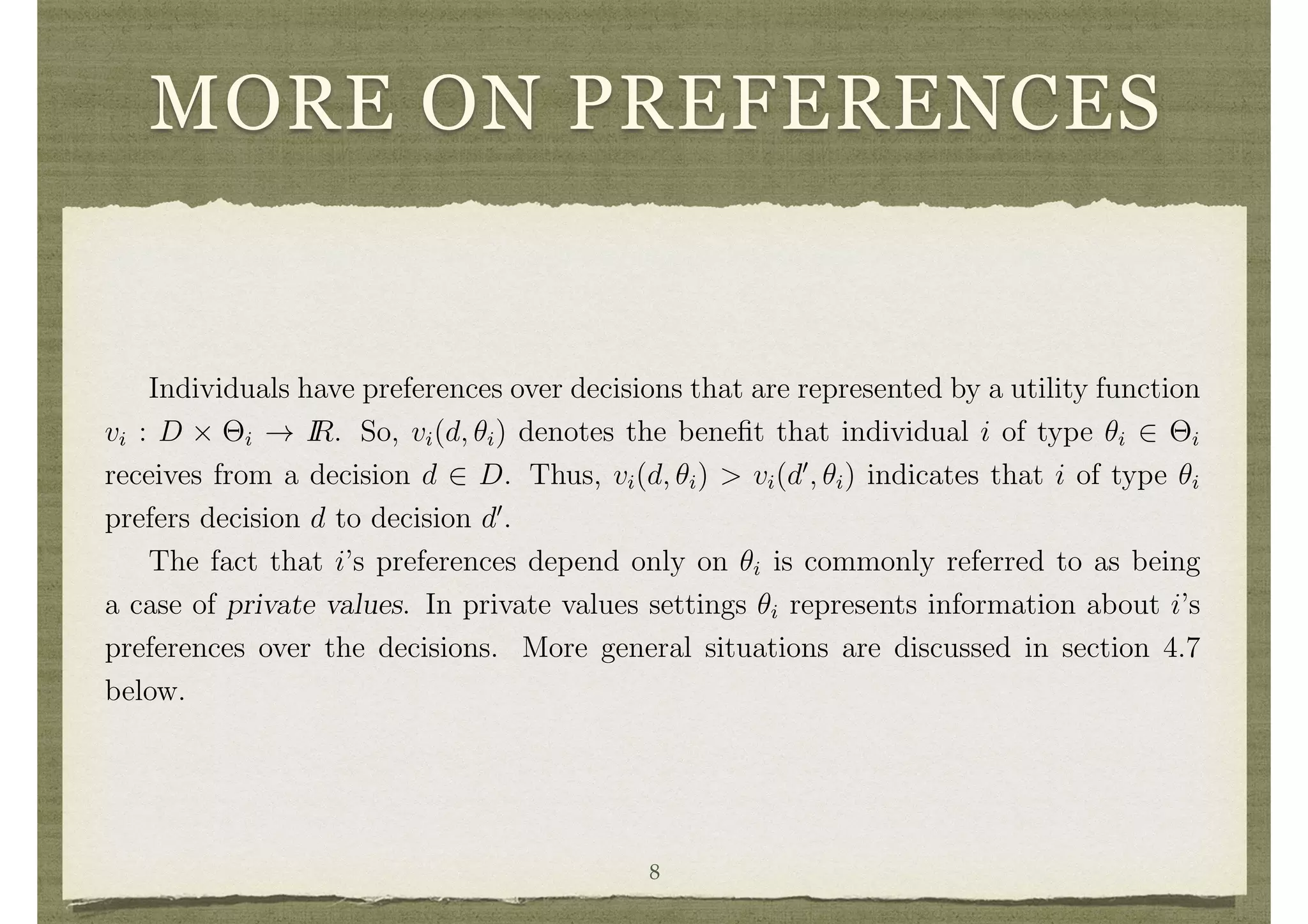
The document summarizes Matthew O. Jackson's 2014 work on mechanism design, which explores the systematic design of institutions and their effects on decision-making among strategically acting individuals with private information. Key concepts include dominant strategy mechanism design, Bayesian mechanism design, and the role of transfer functions in ensuring participation and efficiency in decision-making processes. The paper emphasizes the challenges of achieving both incentive compatibility and efficient outcomes in various settings, while also providing illustrative examples of public and private goods.


![Tom[unit 1]](https://cdn.slidesharecdn.com/ss_thumbnails/tomunit-1-140122191249-phpapp02-thumbnail.jpg?width=640&height=640&fit=bounds)

![[10] degrees of freedom assignment](https://cdn.slidesharecdn.com/ss_thumbnails/10degreesoffreedomassignment-160926065131-thumbnail.jpg?width=640&height=640&fit=bounds)


![[ICF2020]資料](https://cdn.slidesharecdn.com/ss_thumbnails/icf2020ss-210214133513-thumbnail.jpg?width=640&height=640&fit=bounds)


