Download as PDF, PPTX
![Single Potential Buyer
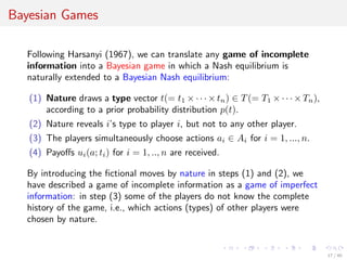
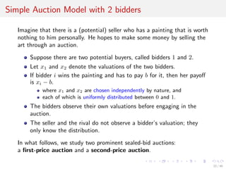
A seller seeks to sell a single indivisible good to a potential buyer.
The buyer’s utility if she purchases the good and pays a monetary
transfer t to the seller is θ − t.
If she does not purchase the good, her utility is zero.
θ is the buyer’s valuation of the good, also called her type.
The seller has a subjective probability distribution over possible
values of θ ∈ [θ, θ]: cdf is denoted by F with density f.
Assume positive support: f(θ) > 0 for all θ ∈ [θ, θ].
£
¢
¡Rm What is an optimal selling mechanism? Is his expected revenue
maximized by committing to a price, as well as by committing to selling
the good at that price whenever the buyer is willing to pay the price?
8 / 40](https://image.slidesharecdn.com/auction-160927005422/85/Introduction-to-Auction-Theory-8-320.jpg)
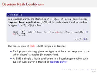
![Fixed Pricing Mechanism
Pick a price p and to say to the buyer that she can have the good if and
only if she is willing to pay p. (Assume the seller can commit to it)
Note that the probability that the buyer’s value is below p is F(p).
The seller’s optimization problem is just the monopoly problem with
demand function 1 − F(p), that is, maxp p(1 − F(p)).
In general, the seller may commit to a direct mechanism (q, t) in which
The buyer is asked to report her type, if it is θ then
Transfer the good to the buyer with probability q(θ), and
The buyer has to pay the seller t(θ).
Definition 2 (Def 2.1)
A direct mechanism consists of functions q and t where
q : [θ, θ] → [0, 1] and t : [θ, θ] → R.
9 / 40](https://image.slidesharecdn.com/auction-160927005422/85/Introduction-to-Auction-Theory-9-320.jpg)
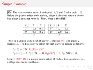
![Revelation Principle (Single Buyer Version)
Theorem 3 (Prop 2.1 – Revelation Principle)
For every mechanism Γ and every optimal buyer strategy σ in Γ, there is
a direct mechanism Γ and an optimal buyer strategy σ in Γ such that
(i) The strategy σ satisfies σ (θ) = θ for every θ ∈ [θ, θ], that is, σ
prescribes telling the truth.
(ii) For every θ ∈ [θ, θ] the probability q(θ) and the payment t(θ) under
Γ equal the probability of purchase and the expected payment that
result under Γ if the buyer plays her optimal strategy σ.
Proof.
For every θ ∈ [θ, θ] define q(θ) and t(θ) as required by (ii) in Theorem 3.
The optimality of truthfully reporting θ in Γ then follows immediately
from the optimality of σ(θ) in Γ.
(← If reporting θ = θ in Γ is strictly better, then choosing σ(θ ) in Γ
must also be better, contradicting to the optimality of σ).
10 / 40](https://image.slidesharecdn.com/auction-160927005422/85/Introduction-to-Auction-Theory-10-320.jpg)
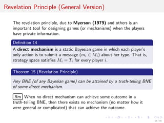
![The Buyer’s Incentive Conditions (1)
Given a direct mechanism, we define the buyer’s expected utility u(θ)
conditional on her type being θ by
u(θ) = θq(θ) − t(θ).
Definition 4 (Def 2.2 and 2.3)
A direct mechanism is incentive compatible if truth telling is optimal
for every θ ∈ [θ, θ], that is, if
u(θ) ≥ θq(θ ) − t(θ ) for all θ, θ ∈ [θ, θ].
A direct mechanism is individually rational if the buyer, conditional on
her type, is willing to participate, that is, if
u(θ) ≥ 0 for all θ ∈ [θ, θ].
11 / 40](https://image.slidesharecdn.com/auction-160927005422/85/Introduction-to-Auction-Theory-11-320.jpg)
![Payoff and Revenue Equivalence
Lemma 6 and the fundamental theorem of calculus implies Lemma 7.
Lemma 7 (Lem 2.3 – Payoff Equivalence)
Consider an incentive compatible direct mechanism. Then for all
θ ∈ [θ, θ] we have
u(θ) = u(θ) +
θ
θ
q(x)dx.
Since u(θ) = θq(θ) − t(θ), we also obtain the following.
Lemma 8 (Lem 2.4 – Revenue Equivalence)
Consider an incentive compatible direct mechanism. Then for all
θ ∈ [θ, θ] we have
t(θ) = t(θ) + (θq(θ) − θq(θ)) −
θ
θ
q(x)dx.
13 / 40](https://image.slidesharecdn.com/auction-160927005422/85/Introduction-to-Auction-Theory-13-320.jpg)
![Characterizing Optimal Mechanism
Theorem 9 (Prop 2.2)
A direct mechanism (q, t) is incentive compatible if and only if
(i) q is increasing.
(ii) For every θ ∈ [θ, θ] we have
t(θ) = t(θ) + (θq(θ) − θq(θ)) −
θ
θ
q(x)dx.
Theorem 10 (Prop 2.3)
An incentive compatible direct mechanism is individually rational if and
only if u(θ) ≥ 0 or equivalently t(θ) ≤ θq(θ).
Lemma 11 (Lem 2.5)
If an incentive compatible and individually rational direct mechanism
maximizes the seller’s expected revenue, then t(θ) = θq(θ).
14 / 40](https://image.slidesharecdn.com/auction-160927005422/85/Introduction-to-Auction-Theory-14-320.jpg)
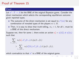
![Proof of Theorem 9
Proof.
Since necessity has been shown, we only need to prove sufficiency. That
is, we have to show u(θ) ≥ θq(θ ) − t(θ ) for any θ, θ ∈ [θ, θ].
u(θ) = θq(θ) − t(θ) ≥ θq(θ ) − t(θ )
⇐⇒
θ
θ
q(x)dx ≥
θ
θ
q(x)dx + (θ − θ )q(θ )
⇐⇒
θ
θ
q(x)dx ≥
θ
θ
q(θ )dx ⇐⇒
θ
θ
(q(x) − q(θ ))dx ≥ 0.
When q is increasing, the last inequality always holds for any θ = θ.
Using Theorem 9 and Lemma 11, the seller can restrict his attention on
the set of all increasing functions q : [θ, θ] → [0, 1].
← Note that t(·) is completely determined by q(·).
15 / 40](https://image.slidesharecdn.com/auction-160927005422/85/Introduction-to-Auction-Theory-15-320.jpg)
![Optimal Selling Mechanism
Extreme point theorem guarantees that the seller can restrict his
attention to non-stochastic mechanisms.
Non-stochastic mechanism is monotone if and only if there is some
p∗
∈ [θ, θ] such that q(θ) = 0 if θ < p∗
and q(θ) = 1 if θ > p∗
.
The seller cannot do better than quoting a simple price p∗
to the
buyer (and the buyer either accepting or rejecting p∗
).
Theorem 12 (Prop 2.5)
The following direct mechanism maximizes the seller’s expected revenues
among all incentive compatible, individually rational direct mechanisms.
Suppose p∗
∈ arg maxp∈[θ,θ] p(1 − F(p)). Then,
q(θ) = 1 if θ ≥ p∗
, and q(θ) = 0 if θ < p∗
,
t(θ) = p∗
if θ ≥ p∗
, and t(θ) = 0 if θ < p∗
.
If there are multiple potential buyers, we consider competitive bidding,
i.e., strategic interactions among buyers must be incorporated.
16 / 40](https://image.slidesharecdn.com/auction-160927005422/85/Introduction-to-Auction-Theory-16-320.jpg)
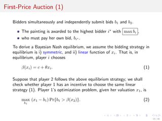
![First-Price Auction (2)
Since x2 is uniformly distributed on [0, 1] by assumption, we obtain
Pr{b1 > β(x2)} = Pr{b1 > c + θx2}
= Pr
b1 − c
θ
> x2 =
b1 − c
θ
.
The first equality comes from the linear bidding strategy (1), the third
equality is from the uniform distribution. Substituting it into (2), the
expected payoff becomes a quadratic function of b1.
max
b1
(x1 − b1)
b1 − c
θ
Taking the first order condition, we obtain
du1
db1
=
1
θ
[−2b1 + x1 + c] = 0 ⇒ b1 =
c
2
+
x1
2
. (3)
Comparing (3) with (1), we can conclude that c = 0 and θ = 1
2
constitute a Bayesian Nash equilibrium.
24 / 40](https://image.slidesharecdn.com/auction-160927005422/85/Introduction-to-Auction-Theory-24-320.jpg)
![Expectation (1)
Definition 17
Given a random variable X taking on values in [0, ω], its cumulative
distribution function (CDF) F : [0, ω] → [0, 1] is:
F(x) = Pr[X ≤ x]
the probability that X takes on a value not exceeding x.
We assume that F is increasing and continuously differentiable.
Definition 18
If X is distributed according to F, then its expectation is
E[X] =
ω
0
xf(x)dx =
ω
0
xdF(x)
and for γ : [0, ω] → R, the expectation of γ(X) is analogously defined as
E[γ(X)] =
ω
0
γ(x)f(x)dx =
ω
0
γ(x)dF(x) .
26 / 40](https://image.slidesharecdn.com/auction-160927005422/85/Introduction-to-Auction-Theory-26-320.jpg)
![Expectation (2)
Definition 19
The conditional expectation of X given that X < x is
E[X | X < x] =
1
F(x)
x
0
tf(t)dt,
which can be rewritten as follows (by integrating by parts):
F(x)E[X | X < x] =
x
0
tf(t)dt
= xF(x) −
x
0
F(t)dt.
The conditional expectation of γ(X) is defined as
E[γ(X) | X < x] =
1
F(x)
x
0
γ(t)f(t)dt.
27 / 40](https://image.slidesharecdn.com/auction-160927005422/85/Introduction-to-Auction-Theory-27-320.jpg)
![Expected Revenue: First-Price
In a first-price auction, the payment is max{1
2 X1, 1
2 X2} .
Recall that β(xi) = 1
2 xi is a BNE.
max{1
2 X1, 1
2 X2} = 1
2 max{X1, X2} = 1
2 Y1.
The expectation of Y1 becomes
E[Y1] =
1
0
yf1(y)dy
=
1
0
2y2
dy =
2
3
y3
1
0
=
2
3
.
The expected revenue of the first-price auction is
1
3
(= 1
2 × 2
3 ).
29 / 40](https://image.slidesharecdn.com/auction-160927005422/85/Introduction-to-Auction-Theory-29-320.jpg)
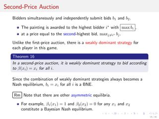
![Expected Revenue: Second-Price
In a second-price auction, the payment is min{X1, X2} .
Recall that β(xi) = xi, i.e., trugh-telling is a BNE.
min{X1, X2} = Y2.
The expectation of Y2 becomes
E[Y2] =
1
0
yf2(y)dy
=
1
0
y × 2(1 − y)dy =
1
0
2(y − y2
)dy
= 2
1
2
y2
1
0
−
1
3
y3
1
0
=
1
3
.
The expected revenue of the second-price auction is
1
3
, which is identical
to the expected revenue of the first-price auction!.
30 / 40](https://image.slidesharecdn.com/auction-160927005422/85/Introduction-to-Auction-Theory-30-320.jpg)
![First-Price: General Model with n bidders (2)
Since (4) holds in equilibrium, i.e., b = β(x),
g(x)
β (x)
(x − b) − G(x) = 0 ⇐⇒ G(x)β (x) + g(x)β(x) = xg(x),
which yields the differential equation
d
dx
(G(x)β(x)) = xg(x).
Taking integral between 0 and x, we obtain
x
0
d
dy
(G(y)β(y))dy = G(x)β(x) − G(0)β(0) =
x
0
yg(y)dy
⇒ β(x) =
1
G(x)
x
0
yg(y)dy = E[Y n−1
1 | Y n−1
1 < x].
£
¢
¡Rm The equilibrium strategy is to bid the the conditional expectation
of second-highest value given that my value x is the highest.
33 / 40](https://image.slidesharecdn.com/auction-160927005422/85/Introduction-to-Auction-Theory-33-320.jpg)
![First-Price: General Model with n bidders (3)
The expected payment (to the seller) of each bidder given x is
G(x) × E[Y n−1
1 | Y n−1
1 < x],
which is identical to that of the second-price auction.
£
¢
¡Rm The expected revenue is just the aggregation of the expected
payment of all bidders, it can be derived by
n ×
ω
0
G(x) × E[Y n−1
1 | Y n−1
1 < x]f(x)dx
= n
ω
0
G(x) ×
1
G(x)
x
0
yg(y)dy f(x)dx
= n
ω
0
x
0
yg(y)dy f(x)dx = n
ω
0
ω
y
f(x)dx yg(y)dy
= n
ω
0
y(1 − F(y))g(y)dy =
ω
0
yf2(y)dy
⇒ E[Y n
2 ] since f2(y) = n(1 − F(y))fn−1
1 (y).
34 / 40](https://image.slidesharecdn.com/auction-160927005422/85/Introduction-to-Auction-Theory-34-320.jpg)
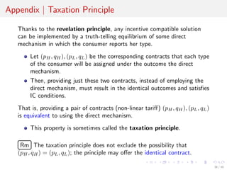

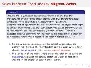
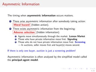
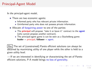
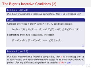
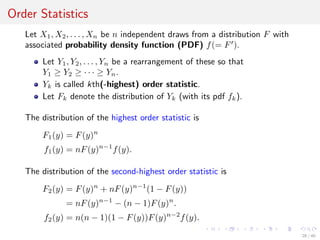
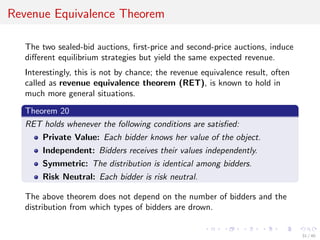
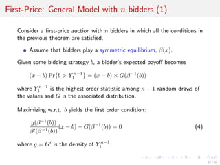
The document comprises lecture slides on auction theory by Yosuke Yasuda from Osaka University, focusing on key concepts such as the independent private values model, conclusions by Milgrom and Weber, and the principal-agent model. It outlines various auction mechanisms, the equivalence of auction forms, revenue maximization strategies, and insights into Bayesian games and the revelation principle. Overall, the lecture emphasizes the mathematical foundations and strategic considerations underlying auction theory and economic mechanisms.


![[ICF2020]資料](https://cdn.slidesharecdn.com/ss_thumbnails/icf2020ss-210214133513-thumbnail.jpg?width=640&height=640&fit=bounds)


