Download as PDF, PPTX


![Framework – some observations
Individual preferences depend only on the rate of substitution:
r =
vK
vM
.
It will turn out that this implies that it is wlog to consider mechanisms
whose outcomes only depend on r. Let:
r ∼ Gj with positive density gj on [rj, r̄j].](https://image.slidesharecdn.com/presentation-220825151659-0811a3d9/85/Redistribution-through-Markets-37-320.jpg)
![Framework – some observations
Individual preferences depend only on the rate of substitution:
r =
vK
vM
.
It will turn out that this implies that it is wlog to consider mechanisms
whose outcomes only depend on r. Let:
r ∼ Gj with positive density gj on [rj, r̄j].
Social preferences can also be expressed as a function of r:
µEB
[xB
K · vK + xB
M · vM ] + ES
[xS
K · vK + xS
M · vM ].](https://image.slidesharecdn.com/presentation-220825151659-0811a3d9/85/Redistribution-through-Markets-38-320.jpg)
![Framework – some observations
Individual preferences depend only on the rate of substitution:
r =
vK
vM
.
It will turn out that this implies that it is wlog to consider mechanisms
whose outcomes only depend on r. Let:
r ∼ Gj with positive density gj on [rj, r̄j].
Social preferences can also be expressed as a function of r:
µEB
vM
xB
K ·
vK
vM
+ xB
M
+ ES
vM
xS
K ·
vK
vM
+ xS
M
.](https://image.slidesharecdn.com/presentation-220825151659-0811a3d9/85/Redistribution-through-Markets-39-320.jpg)
![Framework – some observations
Individual preferences depend only on the rate of substitution:
r =
vK
vM
.
It will turn out that this implies that it is wlog to consider mechanisms
whose outcomes only depend on r. Let:
r ∼ Gj with positive density gj on [rj, r̄j].
Social preferences can also be expressed as a function of r:
µEB
EB
[vM |r]
xB
K · r + xB
M
+ ES
ES
[vM |r]
xS
K · r + xS
M
.](https://image.slidesharecdn.com/presentation-220825151659-0811a3d9/85/Redistribution-through-Markets-40-320.jpg)
![Framework – some observations
Individual preferences depend only on the rate of substitution:
r =
vK
vM
.
It will turn out that this implies that it is wlog to consider mechanisms
whose outcomes only depend on r. Let:
r ∼ Gj with positive density gj on [rj, r̄j].
Social preferences can also be expressed as a function of r:
µEB
EB
[vM |r]
| {z }
λB(r)
xB
K · r + xB
M
| {z }
UB(r)
+ ES
ES
[vM |r]
| {z }
λS(r)
xS
K · r + xS
M
| {z }
US(r)
.](https://image.slidesharecdn.com/presentation-220825151659-0811a3d9/85/Redistribution-through-Markets-41-320.jpg)
![Framework – some observations
Individual preferences depend only on the rate of substitution:
r =
vK
vM
.
It will turn out that this implies that it is wlog to consider mechanisms
whose outcomes only depend on r. Let:
r ≡ vK/vM ∼ Gj with positive density gj on [rj, r̄j].
Social preferences can also be expressed as a function of r:
TS(Λ) = µ
Z r̄B
rB
λB(r)UB(r)dGB(r) +
Z r̄S
rS
λS(r)US(r)dGS(r).](https://image.slidesharecdn.com/presentation-220825151659-0811a3d9/85/Redistribution-through-Markets-42-320.jpg)


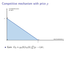
![Single-price mechanisms – seller side
Problem: Choose a price pS to maximize seller welfare while buying
quantity Q and not exceeding a budget of R (where R QG−1
S (Q)).
max
pS≥G−1
S (Q)
(
Q
GS(pS)
Z pS
rS
λS(r)(pS − r)dGS(r) + ΛS(R − pSQ)
)
,
where ΛS = ES[vM ].](https://image.slidesharecdn.com/presentation-220825151659-0811a3d9/85/Redistribution-through-Markets-56-320.jpg)
![Single-price mechanisms – seller side
Problem: Choose a price pS to maximize seller welfare while buying
quantity Q and not exceeding a budget of R (where R QG−1
S (Q)).
max
pS≥G−1
S (Q)
(
Q
GS(pS)
Z pS
rS
λS(r)(pS − r)dGS(r) + ΛS(R − pSQ)
)
,
where ΛS = ES[vM ].
We will refer to the price pC
S = G−1
S (Q) as the competitive price;
Any price pS pC
S leads to rationing.](https://image.slidesharecdn.com/presentation-220825151659-0811a3d9/85/Redistribution-through-Markets-57-320.jpg)


![Single-price mechanisms – seller side
Intuition: There are three effects associated with raising the price pS
above the competitive level pC
S :
1 Allocative efficiency is reduced ↓
2 The mechanism uses up more money leaving a smaller amount
R − pSQ to be redistributed as a lump-sum transfer to all sellers ↓
3 Sellers that sell receive a higher price ↑
Consider the net redistribution effect 2+3:
−ΛS + ES
[λS(r)|r ≤ pS]](https://image.slidesharecdn.com/presentation-220825151659-0811a3d9/85/Redistribution-through-Markets-68-320.jpg)
![Single-price mechanisms – seller side
Intuition: There are three effects associated with raising the price pS
above the competitive level pC
S :
1 Allocative efficiency is reduced ↓
2 The mechanism uses up more money leaving a smaller amount
R − pSQ to be redistributed as a lump-sum transfer to all sellers ↓
3 Sellers that sell receive a higher price ↑
Consider the net redistribution effect 2+3:
−ΛS + ES
[λS(r)|r ≤ pS] ≥ 0 ↑](https://image.slidesharecdn.com/presentation-220825151659-0811a3d9/85/Redistribution-through-Markets-69-320.jpg)
![Single-price mechanisms – seller side
Intuition: There are three effects associated with raising the price pS
above the competitive level pC
S :
1 Allocative efficiency is reduced ↓
2 The mechanism uses up more money leaving a smaller amount
R − pSQ to be redistributed as a lump-sum transfer to all sellers ↓
3 Sellers that sell receive a higher price ↑
Consider the net redistribution effect 2+3:
−ΛS + ES
[λS(r)|r ≤ pS] ≥ 0 ↑
This net effect must be stronger than the negative effect 1 to justify
rationing:
High seller-side inequality;
Low volume of trade: Q Q̄.](https://image.slidesharecdn.com/presentation-220825151659-0811a3d9/85/Redistribution-through-Markets-70-320.jpg)


![Single-price mechanisms – buyer side
Problem: Choose a price pB to maximize buyer welfare while selling
quantity Q and raising a revenue of R (where R QG−1
B (1 − Q)).
max
pB≤G−1
B (1−Q)
Q
1 − GB(pB)
Z r̄B
pB
λB(r)(r − pB)dGB(r) + ΛB(pBQ − R)
.
where ΛB = EB[vM ].](https://image.slidesharecdn.com/presentation-220825151659-0811a3d9/85/Redistribution-through-Markets-73-320.jpg)
![Single-price mechanisms – buyer side
Problem: Choose a price pB to maximize buyer welfare while selling
quantity Q and raising a revenue of R (where R QG−1
B (1 − Q)).
max
pB≤G−1
B (1−Q)
Q
1 − GB(pB)
Z r̄B
pB
λB(r)(r − pB)dGB(r) + ΛB(pBQ − R)
.
where ΛB = EB[vM ].
We will refer to the price pC
B = G−1
B (1 − Q) as the competitive price;
Any price pB pC
B leads to rationing.](https://image.slidesharecdn.com/presentation-220825151659-0811a3d9/85/Redistribution-through-Markets-74-320.jpg)


![Single-price mechanisms – buyer side
Intuition: There are three effects associated with lowering the price pB
below the competitive level pC
B:
1 Allocative efficiency is reduced ↓
2 The mechanism generates less revenue pBQ − R that can be
redistributed as a lump-sum transfer to all buyers ↓
3 Buyers that buy pay a lower price ↑
Consider the net redistribution effect 2+3:
−ΛB + EB
[λB(r)|r ≥ pB]](https://image.slidesharecdn.com/presentation-220825151659-0811a3d9/85/Redistribution-through-Markets-81-320.jpg)
![Single-price mechanisms – buyer side
Intuition: There are three effects associated with lowering the price pB
below the competitive level pC
B:
1 Allocative efficiency is reduced ↓
2 The mechanism generates less revenue pBQ − R that can be
redistributed as a lump-sum transfer to all buyers ↓
3 Buyers that buy pay a lower price ↑
Consider the net redistribution effect 2+3:
−ΛB + EB
[λB(r)|r ≥ pB] ≤ 0 ↓](https://image.slidesharecdn.com/presentation-220825151659-0811a3d9/85/Redistribution-through-Markets-82-320.jpg)
![Single-price mechanisms – buyer side
Intuition: There are three effects associated with lowering the price pB
below the competitive level pC
B:
1 Allocative efficiency is reduced ↓
2 The mechanism generates less revenue pBQ − R that can be
redistributed as a lump-sum transfer to all buyers ↓
3 Buyers that buy pay a lower price ↑
Consider the net redistribution effect 2+3:
−ΛB + EB
[λB(r)|r ≥ pB] ≤ 0 ↓
The net redistribution effect is negative!](https://image.slidesharecdn.com/presentation-220825151659-0811a3d9/85/Redistribution-through-Markets-83-320.jpg)


![Two-price mechanisms – buyer side
Low buyer-side inequality ⇐⇒ λB(rB) ≤ 2ΛB.
Proposition
When buyer-side inequality is low, it is optimal not to offer the low price
pL
B and to choose pH
B = pC
B.
When buyer-side inequality is high, there exists Q ∈ (0, 1] such that
Rationing at the low price is optimal when Q Q;
Setting pH
B = pC
B (and not offering the low price pL
B) is optimal for
Q ≤ Q.](https://image.slidesharecdn.com/presentation-220825151659-0811a3d9/85/Redistribution-through-Markets-94-320.jpg)
![Two-price mechanisms – buyer side
Low buyer-side inequality ⇐⇒ λB(rB) ≤ 2ΛB.
Proposition
When buyer-side inequality is low, it is optimal not to offer the low price
pL
B and to choose pH
B = pC
B.
When buyer-side inequality is high, there exists Q ∈ (0, 1] such that
Rationing at the low price is optimal when Q Q;
Setting pH
B = pC
B (and not offering the low price pL
B) is optimal for
Q ≤ Q.
This is in fact the optimal mechanism overall!](https://image.slidesharecdn.com/presentation-220825151659-0811a3d9/85/Redistribution-through-Markets-95-320.jpg)
![Two-price mechanisms – buyer side
Intuition: This time rationing (a discounted price) is offered to buyers
with relatively low types r ∈ [pL
B, rδ], so that it is possible that the net
redistribution effect is positive:
−ΛB](https://image.slidesharecdn.com/presentation-220825151659-0811a3d9/85/Redistribution-through-Markets-96-320.jpg)
![Two-price mechanisms – buyer side
Intuition: This time rationing (a discounted price) is offered to buyers
with relatively low types r ∈ [pL
B, rδ], so that it is possible that the net
redistribution effect is positive:
−ΛB + EB
[λB(r)| r ∈ [pL
B, rδ]]](https://image.slidesharecdn.com/presentation-220825151659-0811a3d9/85/Redistribution-through-Markets-97-320.jpg)
![Two-price mechanisms – buyer side
Intuition: This time rationing (a discounted price) is offered to buyers
with relatively low types r ∈ [pL
B, rδ], so that it is possible that the net
redistribution effect is positive:
−ΛB + EB
[λB(r)| r ∈ [pL
B, rδ]] ≥ 0](https://image.slidesharecdn.com/presentation-220825151659-0811a3d9/85/Redistribution-through-Markets-98-320.jpg)
![Two-price mechanisms – buyer side
Intuition: This time rationing (a discounted price) is offered to buyers
with relatively low types r ∈ [pL
B, rδ], so that it is possible that the net
redistribution effect is positive:
−ΛB + EB
[λB(r)| r ∈ [pL
B, rδ]] ≥ 0 ↑](https://image.slidesharecdn.com/presentation-220825151659-0811a3d9/85/Redistribution-through-Markets-99-320.jpg)
![Two-price mechanisms – buyer side
Intuition: This time rationing (a discounted price) is offered to buyers
with relatively low types r ∈ [pL
B, rδ], so that it is possible that the net
redistribution effect is positive:
−ΛB + EB
[λB(r)| r ∈ [pL
B, rδ]] ≥ 0 ↑
This net effect must be stronger than the negative effect on allocative
efficiency to justify rationing:
High buyer-side inequality;
High volume of trade: Q Q.](https://image.slidesharecdn.com/presentation-220825151659-0811a3d9/85/Redistribution-through-Markets-100-320.jpg)


![General Framework
A designer chooses a mechanism to allocate a unit mass of objects to
a unit mass of agents.
Each object has quality q ∈ [0, 1], q is distributed acc. to cdf F.
Each agent is characterized by a type (i, r, λ), where:
i is an observable label, i ∈ I (finite);
r is an unobserved willingness to pay (for quality), r ∈ R+;
λ is an unobserved social welfare weight, λ ∈ R+;
The type distribution is known to the designer.
If (i, r, λ) gets a good with quality q and pays t, her utility is qr − t,
while her contribution to social welfare is λ(qr − t)](https://image.slidesharecdn.com/presentation-220825151659-0811a3d9/85/Redistribution-through-Markets-120-320.jpg)
![General Framework
The designer has access to arbitrary (direct) allocation mechanisms
(Γ, T) where Γ(q|i, r, λ) is the probability that (i, r, λ) gets a good with
quality q or less, and T(i, r, λ) is the associated payment, subject to:
Feasibility: E(i,r,λ) [Γ(q|i, r, λ)] ≥ F(q), ∀q ∈ [0, 1];
IC constraint: Each agent (i, r, λ) reports (r, λ) truthfully;
IR constraint: U(i, r, λ) ≡ r
R
qdΓ(q|i, r, λ) − T(i, r, λ) ≥ 0;
Non-negative transfers: T(i, r, λ) ≥ 0, ∀(i, r, λ).
The designer maximizes, for some constant α ≥ 0, a weighted sum of
revenue and agents’ utilities:
E(i,r,λ) [αT(i, r, λ) + λU(i, r, λ)] .](https://image.slidesharecdn.com/presentation-220825151659-0811a3d9/85/Redistribution-through-Markets-121-320.jpg)


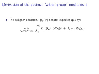
![Framework
Lemma
It is optimal for the designer to condition the allocation and transfers only
on agents’ labels i and WTP r.
Let Vi(r) be the expected per-unit-of-quality social benefit from allocating
a good to an agent with WTP r in group i in an IC mechanism.
With redistributive preferences:
Vi(r) = Λi(r) ·
1 − Gi(r)
gi(r)
| {z }
utility
+ α ·
r −
1 − Gi(r)
gi(r)
| {z }
revenue
where Λi(r) = Er̃∼Gi [ λ | r̃ ≥ r, i].](https://image.slidesharecdn.com/presentation-220825151659-0811a3d9/85/Redistribution-through-Markets-135-320.jpg)
![Framework
Lemma
It is optimal for the designer to condition the allocation and transfers only
on agents’ labels i and WTP r.
Let Vi(r) be the expected per-unit-of-quality social benefit from allocating
a good to an agent with WTP r in group i in an IC mechanism.
With redistributive preferences:
Vi(r) = Λi(r) ·
1 − Gi(r)
gi(r)
| {z }
utility
+ α ·
r −
1 − Gi(r)
gi(r)
| {z }
revenue
where Λi(r) = Er̃∼Gi [ λ | r̃ ≥ r, i].](https://image.slidesharecdn.com/presentation-220825151659-0811a3d9/85/Redistribution-through-Markets-136-320.jpg)
![Framework
Economic idea:
The designer assesses the “need” of agents by estimating the unobserved
welfare weights based on the observable (label i) and elicitable (wtp r)
information:
Λi(r) = Er̃∼Gi [ λ | r̃ ≥ r, i].](https://image.slidesharecdn.com/presentation-220825151659-0811a3d9/85/Redistribution-through-Markets-137-320.jpg)
![Framework
Economic idea:
The designer assesses the “need” of agents by estimating the unobserved
welfare weights based on the observable (label i) and elicitable (wtp r)
information:
Λi(r) = Er̃∼Gi [ λ | r̃ ≥ r, i].
Consequence:
The optimal allocation depends on the statistical correlation of labels
and willingness to pay with the unobserved social welfare weights.](https://image.slidesharecdn.com/presentation-220825151659-0811a3d9/85/Redistribution-through-Markets-138-320.jpg)
![Framework
Economic idea:
The designer assesses the “need” of agents by estimating the unobserved
welfare weights based on the observable (label i) and elicitable (wtp r)
information:
Λi(r) = Er̃∼Gi [ λ | r̃ ≥ r, i].
Consequence:
The optimal allocation depends on the statistical correlation of labels
and willingness to pay with the unobserved social welfare weights.
Correlation is likely to be negative (however, the direction and strength
depend on the market context!)](https://image.slidesharecdn.com/presentation-220825151659-0811a3d9/85/Redistribution-through-Markets-139-320.jpg)


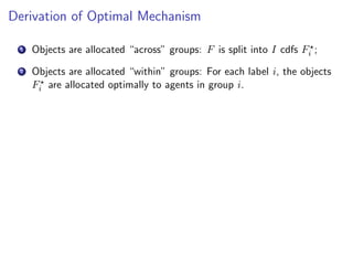


![Derivation of Optimal Mechanism
1 Objects are allocated “across” groups: F is split into I cdfs F⋆
i ;
2 Objects are allocated “within” groups: For each label i, the objects
F⋆
i are allocated optimally to agents in group i.
Observation: Only expected quality, Qi(r), matters for payoffs.
Within a group, agents are partitioned into intervals according to WTP,
with either the “market” or “non-market” allocation in each interval:
Market allocation: assortative matching between WTP and quality
Qi(r) = (F⋆
i )−1
(Gi(r)), ∀r ∈ [a, b];](https://image.slidesharecdn.com/presentation-220825151659-0811a3d9/85/Redistribution-through-Markets-153-320.jpg)
![Derivation of Optimal Mechanism
1 Objects are allocated “across” groups: F is split into I cdfs F⋆
i ;
2 Objects are allocated “within” groups: For each label i, the objects
F⋆
i are allocated optimally to agents in group i.
Observation: Only expected quality, Qi(r), matters for payoffs.
Within a group, agents are partitioned into intervals according to WTP,
with either the “market” or “non-market” allocation in each interval:
Market allocation: assortative matching between WTP and quality
Qi(r) = (F⋆
i )−1
(Gi(r)), ∀r ∈ [a, b];
Non-market allocation: random matching between WTP and quality
Qi(r) = q̄, ∀r ∈ [a, b].
Details](https://image.slidesharecdn.com/presentation-220825151659-0811a3d9/85/Redistribution-through-Markets-154-320.jpg)


![Economic Implications
Assuming differentiability, the condition for using a non-market mechanism
around type r in group i becomes
Λ′
i(r)
1 − Gi(r)
gi(r)
+ α + (Λi(r) − α)
d
dr
1 − Gi(r)
gi(r)
0,
where recall that Λi(r) = Er̃∼Gi [ λ | r̃ ≥ r, i].](https://image.slidesharecdn.com/presentation-220825151659-0811a3d9/85/Redistribution-through-Markets-185-320.jpg)
![Economic Implications
Assuming differentiability, the condition for using a non-market mechanism
around type r in group i becomes
Λ′
i(r)
1 − Gi(r)
gi(r)
+ α + (Λi(r) − α)
d
dr
1 − Gi(r)
gi(r)
0,
where recall that Λi(r) = Er̃∼Gi [ λ | r̃ ≥ r, i].
Thus, non-market allocation is optimal if willingness to pay is strongly
(negatively) correlated with the unobserved social welfare weights.](https://image.slidesharecdn.com/presentation-220825151659-0811a3d9/85/Redistribution-through-Markets-186-320.jpg)
![Economic Implications
Assuming differentiability, the condition for using a non-market mechanism
around type r in group i becomes
Λ′
i(r)
1 − Gi(r)
gi(r)
+ α + (Λi(r) − α)
d
dr
1 − Gi(r)
gi(r)
0,
where recall that Λi(r) = Er̃∼Gi [ λ | r̃ ≥ r, i].
Thus, non-market allocation is optimal if willingness to pay is strongly
(negatively) correlated with the unobserved social welfare weights.
This is more likely to hold when:
The designer has strong redistributive preferences (dispersion in λ’s);
The good being allocated is relatively expensive and everyone needs it;
The label i is not very informative about λ.](https://image.slidesharecdn.com/presentation-220825151659-0811a3d9/85/Redistribution-through-Markets-187-320.jpg)


![Extensions and Future Work
Allocative externalities =⇒ vaccine allocation (ADK + Eric Budish)
Vi(r) = Λi(r) ·
1 − Gi(r)
gi(r)
| {z }
utility
+ α ·
r −
1 − Gi(r)
gi(r)
| {z }
revenue
+ E [Tex|i, r]
| {z }
externality
.](https://image.slidesharecdn.com/presentation-220825151659-0811a3d9/85/Redistribution-through-Markets-217-320.jpg)
![Extensions and Future Work
Allocative externalities =⇒ vaccine allocation (ADK + Eric Budish)
Vi(r) = Λi(r) ·
1 − Gi(r)
gi(r)
| {z }
utility
+ α ·
r −
1 − Gi(r)
gi(r)
| {z }
revenue
+ E [Tex|i, r]
| {z }
externality
.
Pricing versus Rationing](https://image.slidesharecdn.com/presentation-220825151659-0811a3d9/85/Redistribution-through-Markets-218-320.jpg)
![Extensions and Future Work
Allocative externalities =⇒ vaccine allocation (ADK + Eric Budish)
Vi(r) = Λi(r) ·
1 − Gi(r)
gi(r)
| {z }
utility
+ α ·
r −
1 − Gi(r)
gi(r)
| {z }
revenue
+ E [Tex|i, r]
| {z }
externality
.
Pricing versus Rationing versus Queuing (ADK + Shengwu Li)](https://image.slidesharecdn.com/presentation-220825151659-0811a3d9/85/Redistribution-through-Markets-219-320.jpg)
![Extensions and Future Work
Allocative externalities =⇒ vaccine allocation (ADK + Eric Budish)
Vi(r) = Λi(r) ·
1 − Gi(r)
gi(r)
| {z }
utility
+ α ·
r −
1 − Gi(r)
gi(r)
| {z }
revenue
+ E [Tex|i, r]
| {z }
externality
.
Pricing versus Rationing versus Queuing (ADK + Shengwu Li)
vK · xK + vM · xM − vQ · xQ](https://image.slidesharecdn.com/presentation-220825151659-0811a3d9/85/Redistribution-through-Markets-220-320.jpg)
![Extensions and Future Work
Allocative externalities =⇒ vaccine allocation (ADK + Eric Budish)
Vi(r) = Λi(r) ·
1 − Gi(r)
gi(r)
| {z }
utility
+ α ·
r −
1 − Gi(r)
gi(r)
| {z }
revenue
+ E [Tex|i, r]
| {z }
externality
.
Pricing versus Rationing versus Queuing (ADK + Shengwu Li)
vK · xK + vM · xM − vQ · xQ
Other on-going projects:](https://image.slidesharecdn.com/presentation-220825151659-0811a3d9/85/Redistribution-through-Markets-221-320.jpg)
![Extensions and Future Work
Allocative externalities =⇒ vaccine allocation (ADK + Eric Budish)
Vi(r) = Λi(r) ·
1 − Gi(r)
gi(r)
| {z }
utility
+ α ·
r −
1 − Gi(r)
gi(r)
| {z }
revenue
+ E [Tex|i, r]
| {z }
externality
.
Pricing versus Rationing versus Queuing (ADK + Shengwu Li)
vK · xK + vM · xM − vQ · xQ
Other on-going projects:
▶ Application to congestion pricing;](https://image.slidesharecdn.com/presentation-220825151659-0811a3d9/85/Redistribution-through-Markets-222-320.jpg)
![Extensions and Future Work
Allocative externalities =⇒ vaccine allocation (ADK + Eric Budish)
Vi(r) = Λi(r) ·
1 − Gi(r)
gi(r)
| {z }
utility
+ α ·
r −
1 − Gi(r)
gi(r)
| {z }
revenue
+ E [Tex|i, r]
| {z }
externality
.
Pricing versus Rationing versus Queuing (ADK + Shengwu Li)
vK · xK + vM · xM − vQ · xQ
Other on-going projects:
▶ Application to congestion pricing;
▶ Comparison of screening devices.](https://image.slidesharecdn.com/presentation-220825151659-0811a3d9/85/Redistribution-through-Markets-223-320.jpg)


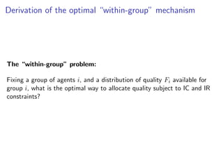


![Derivation of the optimal “within-group” mechanism
The designer’s problem is
max
Ψi
Z 1
0
Vi(t)
z }| {
Z 1
t
Vi(G−1
i (x))dx + max{0, λ̄i − α}ri1{t=0}
dΨi(t)
s.t. Ψi ≻MPS
F−1
i
Agents are partitioned into intervals according to WTP:
▶ Market allocation: assortative matching between WTP and quality
Qi(r) = F−1
i (Gi(r)), ∀r ∈ [a, b];
Back](https://image.slidesharecdn.com/presentation-220825151659-0811a3d9/85/Redistribution-through-Markets-266-320.jpg)
![Derivation of the optimal “within-group” mechanism
The designer’s problem is
max
Ψi
Z 1
0
Vi(t)
z }| {
Z 1
t
Vi(G−1
i (x))dx + max{0, λ̄i − α}ri1{t=0}
dΨi(t)
s.t. Ψi ≻MPS
F−1
i
Agents are partitioned into intervals according to WTP:
▶ Market allocation: assortative matching between WTP and quality
Qi(r) = F−1
i (Gi(r)), ∀r ∈ [a, b];
▶ Non-market allocation: random matching between WTP and quality
Qi(r) = q̄, ∀r ∈ [a, b].
Back](https://image.slidesharecdn.com/presentation-220825151659-0811a3d9/85/Redistribution-through-Markets-267-320.jpg)
![Derivation of the optimal “within-group” mechanism
The designer’s problem is
max
Ψi, F̃i
Z 1
0
Vi(t)
z }| {
Z 1
t
Vi(G−1
i (x))dx + max{0, λ̄i − α}ri1{t=0}
dΨi(t)
s.t. Ψi ≻MPS
F̃−1
i ≻FOSD
F−1
i
Agents are partitioned into intervals according to WTP:
▶ Market allocation: assortative matching between WTP and quality
Qi(r) = F−1
i (Gi(r)), ∀r ∈ [a, b];
▶ Non-market allocation: random matching between WTP and quality
Qi(r) = q̄, ∀r ∈ [a, b].
Back](https://image.slidesharecdn.com/presentation-220825151659-0811a3d9/85/Redistribution-through-Markets-268-320.jpg)

The document discusses inequality-aware market design, emphasizing how market designers consider wealth disparities among participants when creating structures for various markets such as housing, healthcare, and food. It highlights the importance of addressing the equity-efficiency trade-off and the implications of wealth on individuals' preferences and social welfare. Additionally, the paper outlines potential mechanisms for optimal market design that accommodates these inequalities within the constraints of incentive compatibility and budget balance.