The document provides an overview of transport phenomena, emphasizing the unified treatment of momentum, heat, and mass transfer processes relevant to chemical engineering. It outlines course details, including subject focus areas like the Navier-Stokes equations, boundary layer concepts, and various applications, as well as specific problem-solving examples. Recommended textbooks are listed alongside a grading structure based on class tests.


![Equation of Motion –
Navier Stokes equation
/ [ . ]
Dv Dt p g
= − − +
𝜕𝑣𝑥
𝜕𝑥
+
𝜕𝑣𝑦
𝜕𝑦
+
𝜕𝑣𝑧
𝜕𝑧
= 0
𝜌
𝜕 𝑣𝑧
𝜕𝑡
+ 𝑣𝑥
𝜕 𝑣𝑧
𝜕𝑥
+ 𝑣𝑦
𝜕 𝑣𝑧
𝜕𝑦
+ 𝑣𝑧
𝜕 𝑣𝑧
𝜕𝑧
= −
𝜕 𝑃
𝜕𝑧
+ 𝜇
𝜕2 𝑣𝑧
𝜕𝑥2
+
𝜕2 𝑣𝑧
𝜕𝑦2
+
𝜕2 𝑣𝑧
𝜕𝑧2
+ 𝜌 𝑔𝑧
Continuity Equation
Cartesian Coordinate – z component
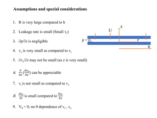
Relevant Boundary Conditions
No slip at the liquid-solid interface
No shear at the liquid-vapor interface
6](https://image.slidesharecdn.com/nsequation-230411195526-db05f2d9/85/NS-Equation-pdf-6-320.jpg)


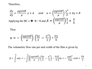


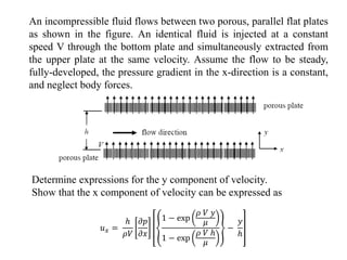


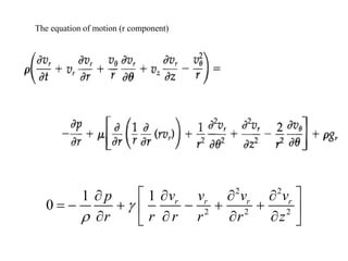


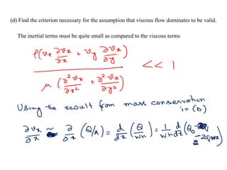
![The mass flow rate versus the pressure drop (W versus ΔP) relationship for a Newtonian
fluid in a circular tube is given by (where ΔP = P0 – PL)
4
4
8
(1)
8
P R P W
W or
L L R
= =
Even for a tapered tue, W does not change with Z
The above equation is assumed to be approximately valid for a differential
length dZ of the tube, whose radius R is slowly changing with Z.
Approximation that a flow between non-parallel surfaces can be treated
locally as a flow between parallel surfaces is know as LUBRICATION
APPROXIMATION.
4
8 1
(2)
[ ( ) ]
d P W
d Z R Z
− =](https://image.slidesharecdn.com/nsequation-230411195526-db05f2d9/85/NS-Equation-pdf-63-320.jpg)
![( )
( )
(3)
o L o
L o
Z
R Z R R R
L
R R
d R
d Z L
= + −
−
=
4
8 1
(2)
[ ( ) ]
d P W
d Z R Z
− =
From Eqns 2 and 3
4
8
L o
W L dR
d P
R R R
− =
−
Integrating the above equation between Z = 0 (R = Ro) and Z = L (R = RL)
4
8
L L
o o
P R
L o
P R
W L dR
d P
R R R
− =
−
](https://image.slidesharecdn.com/nsequation-230411195526-db05f2d9/85/NS-Equation-pdf-64-320.jpg)