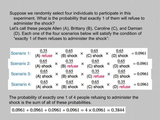
+ 
Binomial distribution 
Slides edited by Valerio Di Fonzo for www.globalpolis.org 
Based on the work of Mine Çetinkaya-Rundel of OpenIntro 
The slides may be copied, edited, and/or shared via the CC BY-SA license 
Some images may be included under fair use guidelines (educational purposes)
Milgram experiment 
Stanley Milgram, a Yale University 
psychologist, conducted a series of 
experiments on obedience to 
authority starting in 1963. 
● Experimenter (E) orders the 
teacher (T), the subject of the 
experiment, to give severe electric 
shocks to a learner (L) each time 
the learner answers a question 
incorrectly. 
● The learner is actually an actor, 
and the electric shocks are not 
real, but a prerecorded sound is 
played each time the teacher 
administers an electric shock. 
http://en.wikipedia.org/wiki/File:Milgram_E 
xperiment_v2.png
Milgram experiment (cont.) 
● These experiments measured the willingness of study 
participants to obey an authority figure who instructed 
them to perform acts that conflicted with their personal 
conscience. 
● Milgram found that about 65% of people would obey 
authority and give such shocks. 
● Over the years, additional research suggested this number 
is approximately consistent across communities and time.
Bernouilli random variables 
● Each person in Milgram's experiment can be thought of as 
a trial. 
● A person is labeled a success if she refuses to administer 
a severe shock, and failure if she administers such shock. 
● Since only 35% of people refused to administer a shock, 
probability of success is p = 0.35. 
● When an individual trial has only two possible outcomes, it 
is called a Bernoulli random variable.
Suppose we randomly select four individuals to participate in this 
experiment. What is the probability that exactly 1 of them will refuse to 
administer the shock? 
Let's call these people Allen (A), Brittany (B), Caroline (C), and Damian 
(D). Each one of the four scenarios below will satisfy the condition of 
“exactly 1 of them refuses to administer the shock”: 
The probability of exactly one 1 of 4 people refusing to administer the 
shock is the sum of all of these probabilities.
Binomial distribution 
The question from the prior slide asked for the probability of 
given number of successes, k, in a given number of trials, n, 
(k = 1 success in n = 4 trials), and we calculated this 
probability as 
# of scenarios x P(single scenario) 
● # of scenarios: there is a less tedious way to figure this 
out, we'll get to that shortly... 
● P(single scenario) = pk(1-p)n-k 
where p is the probability of a success 
The binomial distribution describes the probability of having 
exactly k successes in n independent Bernouilli trials with 
probability of success p.
Computing the # of scenarios 
Earlier we wrote out all possible scenarios that fit the condition 
of exactly one person refusing to administer the shock. If n 
was larger and/or k was different than 1, for example, n = 9 
and k = 2: 
writing out all possible scenarios would be incredibly tedious 
and prone to errors.
Computing the # of scenarios 
Choose function 
The choose function is useful for calculating the number of 
ways to choose k successes in n trials.
Practice 
Which of the following is false?
Binomial distribution (cont.) 
Binomial probabilities 
If p represents probability of success, (1-p) represents 
probability of failure, n represents number of independent 
trials, and k represents number of successes
Binomial conditions 
1. the trials must be independent 
2. the number of trials, n, must be fixed 
3. each trial outcome must be classified as a 
success or a failure 
4. the probability of success, p, must be the 
same for each trial
Practice 
Which of the following is not a condition that needs to be met 
for the binomial distribution to be applicable? 
1. the trials must be independent 
2. the number of trials, n, must be fixed 
3. each trial outcome must be classified as a success 
or a failure 
4. the number of desired successes, k, must be greater than 
the number of trials 
5. the probability of success, p, must be the same for each 
trial
Practice 
According to a 2013 Gallup poll, worldwide only 13% of employees are 
engaged at work (psychologically committed to their jobs and likely to 
be making positive contributions to their organizations). Among a 
random sample of 10 employees, what is the probability that 8 of 
them are engaged at work? 
1. pretty high 
2. pretty low 
We multiple 45 for 
p (*number of probability that 8 
are engaged at work), and 
for 1-p (* 2, which is 10-8, that is 
the probability of non engaged at 
work) 
Gallup: http://www.gallup.com/poll/160061/obesity-rate-stable-2012.aspx, January 23, 2013.
Computing the previous probability in R 
…and with the applet 
http://spark.rstudio.com/minebocek/dist_calc/
Practice 
A 2012 Gallup survey suggests that 26.2% of Americans are 
obese. Among a random sample of 10 Americans, what is 
the probability that exactly 8 are obese?
Expected value 
A 2012 Gallup survey suggests that 26.2% of Americans are 
obese. Among a random sample of 100 Americans, how many 
would you expect to be obese? 
● Easy enough, 100 x 0.262 = 26.2. 
● Or more formally, μ = np = 100 x 0.262 = 26.2. 
● But this doesn't mean in every random sample of 100 people 
exactly 26.2 will be obese. In fact, that's not even possible. In 
some samples this value will be less, and in others more. 
How much would we expect this value to vary?
Expected value and its variability 
Mean and standard deviation of binomial distribution 
Going back to the obesity rate: 
We would expect 26.2 out of 100 randomly sampled Americans 
to be obese, with a standard deviation of 4.4. 
_________ 
Note: Mean and standard deviation of a binomial might not always be 
whole numbers, and that is alright, these values represent what we would 
expect to see on average.
Unusual observations 
Using the notion that observations that are more than 2 
standard deviations away from the mean are considered 
unusual and the mean and the standard deviation we just 
computed, we can calculate a range for the plausible 
number of obese Americans in random samples of 100. 
26.2 ± (2 x 4.4) → (17.4, 35.0)
Normal Approximation to binomial 
FIG. 1 FIG.2 
FIG.3 FIG.4
An analysis of Facebook users 
A recent study found that ``Facebook users get more than they 
give". For example: 
1. 40% of Facebook users in our sample made a friend request, 
but 63% received at least one request 
2. Users in our sample pressed the like button next to friends' 
content an average of 14 times, but had their content ``liked" 
an average of 20 times 
3. Users sent 9 personal messages, but received 12 
4. 12% of users tagged a friend in a photo, but 35% were 
themselves tagged in a photo 
Any guesses for how this pattern can be explained? 
Power users contribute much more content than the typical user. 
http://www.pewinternet.org/Reports/2012/Facebook-users/Summary.aspx
Practice 
This study also found that approximately 25% of Facebook users are 
considered power users. The same study found that the average 
Facebook user has 245 friends. What is the probability that the 
average Facebook user with 245 friends has 70 or more friends who 
would be considered power users? Note any assumptions you must 
make. 
We are given that n = 245, p = 0.25, and we are asked for the 
probability P(K ≥70). To proceed, we need independence, which we'll 
assume but could check if we had access to more Facebook data. 
P(X ≥ 70) = P(K = 70 or K = 71 or K = 72 or … or K = 245) 
= P(K = 70) + P(K = 71) + P(K = 72) + … + P(K = 
245) 
This seems like an awful lot of work...
Normal approximation 
to the binomial
Practice 
What is the probability that the average Facebook user with 
245 friends has 70 or more friends who would be considered 
power users?
Using R for Calculating Binomial 
Distribution 
Why this number is different 
from the previous one? 
Because it is just an 
approximation, and in order to 
reduce the difference, one 
solution is to take out a 0.5 
from the original number (70). 
70
Practice

Binomial distribution

  • 1.
    + Binomial distribution Slides edited by Valerio Di Fonzo for www.globalpolis.org Based on the work of Mine Çetinkaya-Rundel of OpenIntro The slides may be copied, edited, and/or shared via the CC BY-SA license Some images may be included under fair use guidelines (educational purposes)
  • 2.
    Milgram experiment StanleyMilgram, a Yale University psychologist, conducted a series of experiments on obedience to authority starting in 1963. ● Experimenter (E) orders the teacher (T), the subject of the experiment, to give severe electric shocks to a learner (L) each time the learner answers a question incorrectly. ● The learner is actually an actor, and the electric shocks are not real, but a prerecorded sound is played each time the teacher administers an electric shock. http://en.wikipedia.org/wiki/File:Milgram_E xperiment_v2.png
  • 3.
    Milgram experiment (cont.) ● These experiments measured the willingness of study participants to obey an authority figure who instructed them to perform acts that conflicted with their personal conscience. ● Milgram found that about 65% of people would obey authority and give such shocks. ● Over the years, additional research suggested this number is approximately consistent across communities and time.
  • 4.
    Bernouilli random variables ● Each person in Milgram's experiment can be thought of as a trial. ● A person is labeled a success if she refuses to administer a severe shock, and failure if she administers such shock. ● Since only 35% of people refused to administer a shock, probability of success is p = 0.35. ● When an individual trial has only two possible outcomes, it is called a Bernoulli random variable.
  • 5.
    Suppose we randomlyselect four individuals to participate in this experiment. What is the probability that exactly 1 of them will refuse to administer the shock? Let's call these people Allen (A), Brittany (B), Caroline (C), and Damian (D). Each one of the four scenarios below will satisfy the condition of “exactly 1 of them refuses to administer the shock”: The probability of exactly one 1 of 4 people refusing to administer the shock is the sum of all of these probabilities.
  • 6.
    Binomial distribution Thequestion from the prior slide asked for the probability of given number of successes, k, in a given number of trials, n, (k = 1 success in n = 4 trials), and we calculated this probability as # of scenarios x P(single scenario) ● # of scenarios: there is a less tedious way to figure this out, we'll get to that shortly... ● P(single scenario) = pk(1-p)n-k where p is the probability of a success The binomial distribution describes the probability of having exactly k successes in n independent Bernouilli trials with probability of success p.
  • 7.
    Computing the #of scenarios Earlier we wrote out all possible scenarios that fit the condition of exactly one person refusing to administer the shock. If n was larger and/or k was different than 1, for example, n = 9 and k = 2: writing out all possible scenarios would be incredibly tedious and prone to errors.
  • 8.
    Computing the #of scenarios Choose function The choose function is useful for calculating the number of ways to choose k successes in n trials.
  • 9.
    Practice Which ofthe following is false?
  • 10.
    Binomial distribution (cont.) Binomial probabilities If p represents probability of success, (1-p) represents probability of failure, n represents number of independent trials, and k represents number of successes
  • 11.
    Binomial conditions 1.the trials must be independent 2. the number of trials, n, must be fixed 3. each trial outcome must be classified as a success or a failure 4. the probability of success, p, must be the same for each trial
  • 12.
    Practice Which ofthe following is not a condition that needs to be met for the binomial distribution to be applicable? 1. the trials must be independent 2. the number of trials, n, must be fixed 3. each trial outcome must be classified as a success or a failure 4. the number of desired successes, k, must be greater than the number of trials 5. the probability of success, p, must be the same for each trial
  • 13.
    Practice According toa 2013 Gallup poll, worldwide only 13% of employees are engaged at work (psychologically committed to their jobs and likely to be making positive contributions to their organizations). Among a random sample of 10 employees, what is the probability that 8 of them are engaged at work? 1. pretty high 2. pretty low We multiple 45 for p (*number of probability that 8 are engaged at work), and for 1-p (* 2, which is 10-8, that is the probability of non engaged at work) Gallup: http://www.gallup.com/poll/160061/obesity-rate-stable-2012.aspx, January 23, 2013.
  • 14.
    Computing the previousprobability in R …and with the applet http://spark.rstudio.com/minebocek/dist_calc/
  • 15.
    Practice A 2012Gallup survey suggests that 26.2% of Americans are obese. Among a random sample of 10 Americans, what is the probability that exactly 8 are obese?
  • 16.
    Expected value A2012 Gallup survey suggests that 26.2% of Americans are obese. Among a random sample of 100 Americans, how many would you expect to be obese? ● Easy enough, 100 x 0.262 = 26.2. ● Or more formally, μ = np = 100 x 0.262 = 26.2. ● But this doesn't mean in every random sample of 100 people exactly 26.2 will be obese. In fact, that's not even possible. In some samples this value will be less, and in others more. How much would we expect this value to vary?
  • 17.
    Expected value andits variability Mean and standard deviation of binomial distribution Going back to the obesity rate: We would expect 26.2 out of 100 randomly sampled Americans to be obese, with a standard deviation of 4.4. _________ Note: Mean and standard deviation of a binomial might not always be whole numbers, and that is alright, these values represent what we would expect to see on average.
  • 18.
    Unusual observations Usingthe notion that observations that are more than 2 standard deviations away from the mean are considered unusual and the mean and the standard deviation we just computed, we can calculate a range for the plausible number of obese Americans in random samples of 100. 26.2 ± (2 x 4.4) → (17.4, 35.0)
  • 19.
    Normal Approximation tobinomial FIG. 1 FIG.2 FIG.3 FIG.4
  • 20.
    An analysis ofFacebook users A recent study found that ``Facebook users get more than they give". For example: 1. 40% of Facebook users in our sample made a friend request, but 63% received at least one request 2. Users in our sample pressed the like button next to friends' content an average of 14 times, but had their content ``liked" an average of 20 times 3. Users sent 9 personal messages, but received 12 4. 12% of users tagged a friend in a photo, but 35% were themselves tagged in a photo Any guesses for how this pattern can be explained? Power users contribute much more content than the typical user. http://www.pewinternet.org/Reports/2012/Facebook-users/Summary.aspx
  • 21.
    Practice This studyalso found that approximately 25% of Facebook users are considered power users. The same study found that the average Facebook user has 245 friends. What is the probability that the average Facebook user with 245 friends has 70 or more friends who would be considered power users? Note any assumptions you must make. We are given that n = 245, p = 0.25, and we are asked for the probability P(K ≥70). To proceed, we need independence, which we'll assume but could check if we had access to more Facebook data. P(X ≥ 70) = P(K = 70 or K = 71 or K = 72 or … or K = 245) = P(K = 70) + P(K = 71) + P(K = 72) + … + P(K = 245) This seems like an awful lot of work...
  • 22.
  • 23.
    Practice What isthe probability that the average Facebook user with 245 friends has 70 or more friends who would be considered power users?
  • 24.
    Using R forCalculating Binomial Distribution Why this number is different from the previous one? Because it is just an approximation, and in order to reduce the difference, one solution is to take out a 0.5 from the original number (70). 70
  • 25.

Editor's Notes

  • #20 Say we have a binomial random variable with probability of success 0.25. This is what the distribution looks like when n is equal to 10 (fig.1), and each bar represents a potential outcome. With ten trials, the number of successes could range anywhere from 0 to 10 and therefore we have 11 bars here. Heights of the bars represent the likelihood of these outcomes. For example, the probability of zero successes can be calculated as 0.75. The probability of failure raised to the 10th power since zero successes basically means ten failures. This value comes out to be approximately 0.056, which is the height of this bar. With n equals 10 and p equals 0.25, the expected number of successes is 2.5 (indicated by the arrow in the middle), and hence the distribution is centered around this value. So, the binomial distribution, with p equals 0.25 and n equals 10 is right skewed. Keeping p constant at 0.25 and increasing n equals 20 (fig. 2) we see a change in the center of the distribution, which is expected since n times p is now different. But we also see a change in the shape. The distribution, while still right-skewed, is looking much less skewed. Increasing the sample size further to 50 (fig.3), the distribution looks even more symmetric, and much smoother, and increasing the sample size even further to 100 (fig.4), the distribution looks no different than the normal distribution.