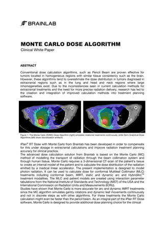
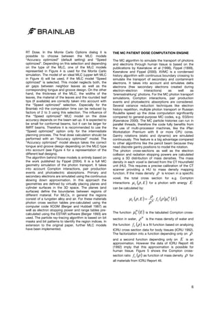
Learn more: https://www.brainlab.com/iplan-rt Conventional dose calculation algorithms, such as Pencil Beam are proven effective for tumors located in homogeneous regions with similar tissue consistency such as the brain. However, these algorithms tend to overestimate the dose distribution in tumors diagnosed in extracranial regions such as in the lung and head and neck regions where large inhomogeneities exist. Due to the inconsistencies seen in current calculation methods for extracranial treatments and the need for more precise radiation delivery, research has led to the creation and integration of improved calculation methods into treatment planning software.

1. MONTE CARLO DOSE ALGORITHM
Clinical White Paper
ABSTRACT
Conventional dose calculation algorithms, such as Pencil Beam are proven effective for
tumors located in homogeneous regions with similar tissue consistency such as the brain.
However, these algorithms tend to overestimate the dose distribution in tumors diagnosed in
extracranial regions such as in the lung and head and neck regions where large
inhomogeneities exist. Due to the inconsistencies seen in current calculation methods for
homogeneities
extracranial treatments and the need for more precise radiation delivery, research has led to
the creation and integration of improved calculation methods into treatmen planning
treatment
software.
Figure 1: The Monte Carlo (XVMC) Dose Algorithm (right) simulates rotational treatments continuously while Semi Analytical Dose
Algorithms (left) show discretization artifacts.
iPlan® RT Dose with Monte Carlo from Brainlab has been developed in order to compensate
for this under dosage in extracranial calculations and improve radiation treatment planning
accuracy for clinical practice.
The advanced dose calculation solution from Brainlab is based on the Monte Carlo (MC)
Brainlab
method of modelling the transport of radiation through the beam collimation system and
through human tissue. Monte Carlo requires a 3-dimensional CT-scan of the patient's tissue
3
scan
to create an internal model of the patient and to calculate the dose distribution of the radiation
patient
emitted by a medical linear accelerator. The present implementation is designed to model
photon radiation. It can be used to calculate dose for conformal Multileaf Collimator (MLC)
treatments including conformal beam, IMRT, static and dynamic arc and HybridArcTM
ing
treatment modalities. The MLC and patient models are created using interaction parameter
tabulations from the National Institute of Standards and Technology (NIST) of the USA and the
International Commission on Radiation Units and Measurements (ICRU).
ional
Studies have shown that Monte Carlo is more accurate for arc and dynamic IMRT treatments
since the MC algorithm simulates gantry rotations and dynamic leaf movements continuously
and not in discrete steps as with other algorithms. For these treatments the Monte Carlo
ete
calculation might even be faster than the pencil beam. As an integral part of the iPlan RT Dose
software, Monte Carlo is designed to provide additional dose planning choice for the clinical
cl

2. practice resulting in more informed treatment options especially for extracranial indications.
This paper introduces the background to the Monte Carlo Dose algorithm and its integration
into Brainlab treatment planning software. It provides an overview of the physical features
behind the iPlan RT Dose Monte Carlo (MC) algorithm and allows the reader to understand the
behavior of the MC algorithm and how it will be integrated into the clinical environment. For
more detailed information about the MC techniques in general and the XVMC algorithm in
particular, refer to the publications listed in section References.
Figure 2: Schematic representation of two particle history examples within the patient model. Illustrated are photons (yellow),
electrons (green) and positrons (red). The red dots represent interactions of the particles with atoms of the tissue.
INTRODUCTION
New cancer treatment techniques like IGRT and IMRT
allow more precise dose deposition in the target
volume and an improved control of the normal tissue
complications. An accurate dose calculation is essential
to assure the quality of the improved techniques.
Conventional dose calculation methods, like the pencil
beam algorithm, are of high quality in regions with
re
homogeneous tissue, e.g. within the brain. However, for
treatments in the head-and-neck or in the thorax
neck
regions, i.e. in regions consisting of bone, soft tissue
and air cavities, an improved accuracy is required. For
example, the pencil beam algorithm is known to
mple,
overestimate the dose in the target volume for the
treatment of small lung tumors. The reason is, the
pencil beam algorithm calculates dose by scaling pencil
beam dose distribution kernels in water to take the
tissue heterogeneities into account, but this method
ssue
has accuracy limitations in these regions. MC dose
calculation algorithms, on the other hand, provide more
accurate results especially in heterogeneous regions.
The MC technique is a stochastic method for solving
complex equations or integrals numerically. MC
techniques are based on pseudo random numbers
generated by computer algorithms called random
number generators. Pseudo random numbers are not
really random; however high quality random number
generators
rators
provide
uniformly
distributed
and
uncorrelated numbers, i.e. they behave like random
numbers. In other words, two arbitrarily generated
pseudo random numbers are independent from each
other.
In radiotherapy MC techniques are applied to solve the
transport problem of ionizing radiation within the human
body. Here the radiation is decomposed into single
quantum particles (photons, electrons, positrons). The
motion of these particles through the irradiation device
and the human tissue is simulated by taking into
account the material properties of the different
components of the Linac head and the tissue properties

3. in each volume element (voxel). The photons, electrons
and positrons interact with the electrons of the atomic
shells and the electromagnetic field of the atomic
nuclei. This can cause ionization events. The
corresponding interaction properties are based on
quantum physics.
For the Linac head these properties can be calculated
using the known atomic composition of the different
components, for the patient they can be calculated
based on the CT images and the Hounsfield Unit in
each voxel. The interaction properties are given as total
and differential cross sections. Total cross sections
characterize the interaction probabilities of a particle
with a given energy in a medium with a definite atomic
composition. Differential cross sections characterize
the probability distribution functions for the generation
of secondary particles with definite secondary particle
parameters like energy and scattering angle. The
random numbers in a MC simulation are required to
sample the specific parameters from these probability
distribution functions. For example, the path length of a
photon with given energy is sampled from an
exponential distribution function based on the linear
attenuation coefficients along the straight line from the
starting position to the interaction point. The type of the
photon interaction (photoelectric absorption, Compton
scatter or pair production) is sampled from the total
cross sections of these processes. After sampling the
secondary particle parameters from the differential
cross sections, the secondary particles are simulated in
a similar manner. This procedure causes a particle
history beginning with an initial particle and many
daughter particles in multiple generations. The process
stops if the remaining energy falls below some
minimum energy (also called cut-off energy) or all
particles have left the region of interest. Figure 2 shows
two examples of possible particle histories.
The MC simulation of charged particles (electrons and
positrons) is more complicated and more time
consuming than the simulation of photons because the
number of interactions per length unit is much higher.
However, the so-called condensed history technique
allows the simulation of charged particles in a
reasonable time. Using this technique a large number of
elastic and semi-elastic interactions is grouped
together into one particle step and is modeled as a
multiple interaction with continuous energy loss of the
electrons and positrons along their paths.
At each charged particle step the amount of absorbed
energy is calculated and accumulated in a threedimensional matrix. Later this matrix is transformed into
dose by dividing the energy in each voxel by the mass
of the voxel. Generally, a huge number of particle
histories must be simulated in a MC calculation.
Otherwise, the number of energy deposition events per
voxel is small. This leads to a large variance of the dose
value in each voxel and the dose distribution becomes
noisy. The effect of noisy dose distributions can be
observed at the iso-dose lines if they appear too
jagged. Sometimes it is difficult to distinguish between
physical and statistical fluctuations. Therefore it is
important to calculate a smooth dose distribution with
small statistical variance. This statistical variance per
voxel decreases with increasing number of histories
N hist
as
1
N hist , i.e. the statistical variance can be
decreased by a factor of 2 if the number of histories is
increased by a factor of 4. This behavior contributes to
the long calculation times of MC algorithms. In general,
MC dose algorithms consist of at least two
components. One component is a virtual model of the
treatment device. It is used as particle source and
provides particle parameter (position, angle, energy,
charge) distributions close to reality. The second
component takes the particles generated by the first
component as input. It models the particle transport
through the patient and calculates the dose distribution.
It is useful to subdivide the first component, the model
of the Linac head, into further subcomponents (see
below).
For a more thorough introduction into all issues
associated with clinical implementation of Monte Carlobased external beam treatment planning we refer to the
review by Reynaert et al (2007) or the AAPM Task
Group Report No 105 (2007).
X-RAY VOXEL MONTE CARLO (XVMC)
The iPlan RT Dose Monte Carlo algorithm is based on
the X-ray Voxel Monte Carlo algorithm developed by
Iwan Kawrakow and Matthias Fippel (Kawrakow et al
1996, Fippel et al 1997, Fippel 1999, Fippel et al 1999,
Kawrakow and Fippel 2000, Fippel et al 2003, Fippel
2004). The XVMC algorithm consists of 3 main
components (see Figure 3).
The first component is used as particle source. It
models the upper part of the Linac head (target,
primary collimator, flattening filter) and generates
photons as well as contaminant electrons from the
corresponding distribution. The particles are then
transferred to the second component, the model of the
collimating system. Depending on the field
configuration, the particles are absorbed, scattered or
passed through. The surviving particles are transferred
to the patient dose computation engine. In this third
component the radiation transport through the patient
geometry is simulated and the dose distribution is
computed. In the following sections the 3 components
of XVMC are characterized in more detail.
THE VIRTUAL ENERGY FLUENCE MODEL
The geometry of the target, the flattening filter and the
primary collimator does not change when the field
3

4. Figure 3: The 3 components of XVMC.
shape is changed. Therefore, it can be assumed that
the phase space of photons and charged particles
above the jaws and the MLC is independent on the field
configuration. To model this phase space, a Virtual
Energy Fluence Model (VEFM) is employed. With some
extensions this model is based on the work by Fippel et
al (2003).
It consists of two or three photon sources with twotwo
dimensional Gaussian shape and one charged particle
sional
(electron) contamination source. The photon sources
model ‘bremsstrahlung’ photons created in the target
and Compton photons scattered by the primary
collimator and flattening filter materials. For the photon
sources various parameters are required. For example,
the distances of the sources to the nominal beam focus
is either estimated or taken from the technical
information provided by Linac vendor. The Gaussian
widths (standard deviations) as well as the rela
relative
weights of the photon sources are fitted using
measured dose distributions in air. Additional horn
correction parameters are also fitted from these
measurements. They model deviations of the beam
profile from an ideal flat profile.
The measurements in air have to be performed by a
qualified medical physicist in the clinic using an empty
water phantom. It is necessary to measure profiles and
in-air output factors (head scatter factors) for a variety
air
of field sizes representing the range of treatment fie
field
sizes. The profiles must be measured in different
directions and with different distances to the beam
focus. It is recommended to use an ionization chamber
with built-up cap for the measurements. The cap
up
increases the number of electrons in the chamber with
the aim of an improved measurement signal. It also
removes electrons coming from the Linac head. The
cap should be as small as possible to guarantee a high
d
spatial resolution. Therefore, it should consist of a
material with high density, e.g. brass or some similar
material. The thickness of the cap is estimated such
that the depth of dose maximum is reached.
The measured profiles are normalized using the in
in-air
output factors. In this way they provide absolute dose
ut
profiles per monitor unit. Then the data can be used as
representation of a photon fluence distribution in air
versus field size. On the other hand, based on the
model assumptions a theoretical fluence dis
distribution in
air can be calculated analytically. By minimizing the
deviations between both distributions, the free model
parameters can be adjusted. The minimization is
performed using a Levenberg-Marquardt algorithm
Levenberg
(Press et al 1992).
The VEFM also requires information about the photon
res
energy spectrum as well as the fluence of charged
particle contamination at the patient’s surface. This
information is derived from a measured depth dose
curve Dmeas z in water for the reference field size
( )
(field size used for the dose – monitor unit calibration).
ield
The curve Dmeas z is used to minimize the squared
( )
difference to a calculated depth dose curve
Based on the model assumptions,
Dcalc ( z ) .
Dcalc ( z )
is given
by:
E max
Dcalc (z ) = wγ
∫ dE p( E ) D (E , z ) + w D (z ).
mono
e
e
E min
4

5. The
set
of
Dmono (E , z )
mono-energetic depth dose curves
in water is calculated using Monte Carlo
and the geometric beam model parameters derived
after fitting the measured profiles in air. The set is
calculated for a table of energies reaching from the
minimum energy of the spectrum
Emin
up to an energy
that is a little larger than the maximum energy
This allows us to use
E max
E max
.
water and the formula on
Dcalc ( z ) .
It requires the
depth dose MC computation of a pure electron
contamination source in water De z . Because most of
( )
the electrons originate in the flattening filter, the
location of the electron source is assumed to be the
foot plane of the filter. The energy spectrum of the
electrons is estimated by an exponential distribution as
described by Fippel et al (2003).
also as a fitting parameter.
In contrast to the original paper (Fippel et al 2003), we
model the energy spectrum
(
p(E ) by:
)
p(E ) = N 1 − e−lE e−bE ,
MODELING OF THE COLLIMATING SYSTEM
Emin ≤ E ≤ Emax .
This function behaves more comparable to spectra
calculated using EGSnrc (Kawrakow 2000) and BEAM
(Rogers et al 1995) especially in the low energy region.
The free parameters l, b and the normalization factor
N
are fitted. For
Emin
and
E max
we usually take fix
values, but it is possible to adjust them also, because
sometimes the maximum energy of the spectrum can
be different from the
nominal photon energy setting in MV. The parameter
wγ
is the total weight of all photon sources. It is
calculated by
wγ = 1 − we
with
we
being the weight
of the electron contamination source. The parameter
we is also fitted using the measured depth dose in
The components of the collimating system (jaws and
MLC) are modeled in different ways. The rectangle
given by the positions of both jaw pairs is used to
define the sampling space of the initial particles. That
means only photons and electrons are generated going
through the jaw opening. In other words, the MC
algorithm assumes fully blocking jaws. The error of this
assumption is estimated to be below 0.5% because of
the jaw thickness and the attenuation of the jaw
material. Furthermore, the beam is additionally blocked
by the MLC leading to further reduction of the photon
fluence outside the beam limits. The advantage of this
approach is that it saves computation time. The
simulation of photon histories being absorbed within
the jaw material would just be a waste of computing
power and it would not have a significant effect on the
calculation accuracy.
The MLC on the other hand can be simulated with two
different precision levels selected by the user of iPlan
Figure 4: Different MLC leaf designs (from upper left to lower right): ideal MLC (no leakage radiation), tilted
leaves (Siemens), step design (Elekta), tongue and groove design (Varian), Varian Millennium, Brainlab m3.
Represented are only 4 leaf pairs per MLC.
5

6. RT Dose. In the Monte Carlo Options dialog it is
possible to choose between the MLC models
“Accuracy optimized” (default setting) and “Speed
optimized”. Depending on this selection and depending
on the type of the MLC, one of the MLC models
represented in Figure 4 is used for the Monte Carlo
simulation. The model of an ideal MLC (upper left MLC
in Figure 4) will be used, if the MLC model “Speed
optimized” is selected. This model neglects both, the
air gaps between neighbor leaves as well as the
corresponding tongue and groove design. On the other
hand, the thickness of the MLC, the widths of the
leaves, the material of the leaves and the rounded leaf
tips (if available) are correctly taken into account with
the “Speed optimized” selection. Especially for the
Brainlab m3 the computation time can be reduced by
factors of 2 to 3 using this selection. The influence of
the “Speed optimized” MLC model on the dose
accuracy depends on the beam set up. It is expected to
be small for conformal beams, but it can be larger for
IMRT beams. Therefore it is recommended to use the
“Speed optimized” option only for the intermediate
planning process. The final dose calculation should be
performed with an “Accuracy optimized” model. The
“Accuracy optimized” model always takes the correct
tongue and groove design depending on the MLC type
into account (see Figure 4 for a representation of the
different leaf designs).
The algorithm behind these models is entirely based on
the work published by Fippel (2004). It is a full MC
geometry simulation of the photon transport. It takes
into account Compton interactions, pair production
events and photoelectric absorptions. Primary and
secondary electrons are simulated using the continuous
slowing down approximation. In this approach the
geometries are defined by virtually placing planes and
cylinder surfaces in the 3D space. The planes (and
surfaces) define the boundaries between regions of
different material. For MLCs, in general the regions
consist of a tungsten alloy and air. For these materials
photon cross section tables pre-calculated using the
computer code XCOM (Berger and Hubbell 1987) as
well as electron stopping power and range tables precalculated using the ESTAR software (Berger 1993) are
used. The particle ray-tracing algorithm is based on bit
masks and bit patterns to identify the region indices. In
extension to the original paper, further MLC models
have been implemented.
THE MC PATIENT DOSE COMPUTATION ENGINE
The MC algorithm to simulate the transport of photons
and electrons through human tissue is based on the
publications by Kawrakow et al (1996), Fippel (1999),
Kawrakow and Fippel (2000). XVMC is a condensed
history algorithm with continuous boundary crossing to
simulate the transport of secondary and contaminant
electrons. It takes into account and simulates delta
electrons (free secondary electrons created during
electron-electron
interactions)
as
well
as
‘bremsstrahlung’ photons. For the MC photon transport
simulations, Compton interactions, pair production
events and photoelectric absorptions are considered.
Several variance reduction techniques like electron
history repetition, multiple photon transport or Russian
Roulette speed up the dose computation significantly
compared to general-purpose MC codes, e.g. EGSnrc
(Kawrakow 2000). The MC particle histories can run in
parallel threads, therefore the code fully benefits from
the use of multi-processor machines, like the iPlan
Workstation Premium with 8 or more CPU cores.
Gantry rotations (static and dynamic) are simulated
continuously. This feature is a big advantage compared
to other algorithms like the pencil beam because they
need discrete gantry positions to model the rotation.
The photon cross-sections as well as the electron
collision and radiation stopping powers are calculated
using a 3D distribution of mass densities. The mass
density in each voxel is derived from the CT Hounsfield
unit (HU). This requires a precise calibration of the CT
scanner providing a HU to mass density mapping
function. If the mass density ρ is known in a specific
voxel, the total cross section for e.g. Compton
interactions µ C ρ , E for a photon with energy E
(
)
can be calculated by:
µ C (ρ , E ) =
The function
W
µC ( E )
is the tabulated Compton cross-
W
ρ is the mass density of water and
f C (ρ ) is a fit function based on analyzing
section in water,
the function
ρ
W
f C (ρ )µ C (E ).
W
ρ
ICRU cross section data for body tissues (ICRU 1992).
The factorization into a function depending only on ρ
and a second function depending only on E is an
approximation. However the data of ICRU Report 46
(1992) imply that this approximation is possible for
human tissue. Figure 5 shows the Compton crosssection ratio f C ρ as function of mass density ρ for
( )
all materials from ICRU Report 46.
6

7. The line in Figure 5 represents a fit to these data. It is
given by:
The function
densities
0.99 + 0.01 ρ ρ , ρ ≤ ρ
f C (ρ ) ≈ 
W
W
0.85 + 0.15 ρ ρ , ρ ≥ ρ
W
W
This fit function is used by XVMC to calculate the
Compton cross-section. There are a few materials with
section.
deviations between the real cross section ratio and the
fit function of up to 1.5%. However, these are materials
like gallstone or urinary stones. Furthermore, the
Furt
correct elemental composition in a given voxel is
unknown. Only a HU number is known and different
material compositions can lead to the same HU.
Therefore, the HU number itself has some uncertainty
overlaying in this manner the uncertainty of the fit
function. The influence of the HU number uncertainty
on Monte Carlo calculated dose distributions has been
discussed in the literature (Vanderstraeten et al 2007).
Similar fit functions exist to calculate the pair
production and photoelectric cross
s-sections as well as
the electron collision and radiation stopping powers.
Their dependencies on the mass density of course
differ from f C ρ .
ρ
f C (ρ )
is also used to convert mass
into electron densities
ne
or vice versa.
The relation is given by:
W
ne = ne
with
W
ne
ρ
f (ρ )
ρW C
being the electron density of water.
( )
Figure 5: Compton cross section ratio versus mass density for all materials of ICRU report 46
cross-section
(crosses). The line represents a fit to these data. This function is used by XVMC to calculate the
Compton cross-section.
section.
7

8. THE MC PARAMETERS
MEAN VARIANCE
Within iPlan RT Dose software the user has some
influence on the MC dose calculation accuracy, the
dose calculation time and the dose result type. This can
be done using the Monte Carlo Options. Four
parameters can be influenced:
The mean variance parameter estimates the number of
particles histories needed to achieve this variance per
beam in % of the maximum dose of that beam.
Because everything here is normalized per beam, the
final variance in the PTV can be smaller. For example, if
we have 5 overlapping beams in the PTV and each
beam is calculated with 2% variance, then the variance
in the PTV is about 1.
In the non-overlapping regions it remains 2%. Because
overlapping
•
•
•
•
Spatial resolution (in mm),
Mean variance (in %),
Dose result type (“Dose to medium” or “Dose
to water”)
MLC model (“Accuracy optimized” or “Speed
optimized”).
of the
1
N hist law mentioned in the introduction, the
calculation time increases by a factor of 4 if the mean
variance is decreased by a factor of 2. The final
calculation should be 1% or smaller.
SPATIAL RESOLUTION
The spatial resolution defines the size of the internal
MC dose computation grid. It does not mean however
es
that the final MC grid size is exactly equal to the value
of the parameter. The MC voxels are constructed by
combining an integer number of pixels from the original
CT cube. Therefore the final sizes of the voxels are only
approximately equal to the value of the spatial
resolution parameter. They can also be different for the
3 spatial directions. Furthermore, they cannot be
smaller than the initial pixel sizes. The selection of this
parameter has a strong influence on the calculation
time. Decreasing this parameter by a factor of 2 can
me.
increase the calculation time by a factor of about 6.
Final dose calculations for small tumors should be
performed with a spatial resolution of 2 to 3 mm.
DOSE RESULT TYPE
The iPlan RT Dose application allows the calculation of
2 different dose types. The default setting “Dose to
medium” means real energy dose, i.e. the energy
absorbed in a small tissue element divided by the mass
of the tissue element. “Dose to water”, on the other
hand, means energy absorbed in a small cavity of water
divided by the mass of that cavity, whereas some
tissue, e.g. bone, surrounds the cavity (see Figure 6).
rrounds
There is no visible difference between “Dose to
medium” and “Dose to water” for most of the human
soft tissue types. However, “Dose to water” can be up
to 15% larger compared to “Dose to medium” for bony
tissues (AAPM 2007). This is because of the high
high-
Figure 6: The difference between “Dose to medium” and “Dose to water”. “Dose to medium” should be calculated if
the user is interested in the average dose within the whole voxel. “Dose to water” should be calculated if the user has
more interest in the dose within small soft tissue cells surrounded by bone material.
s
8

9. density bone causing a higher fluence of secondary
electrons in the water cavity and accordingly causing a
higher dose compared to the case of the cavity filled
also with bone. Therefore “Dose to water” should be
selected if the user wants to know the dose in soft
tissue cells within a bony structure (see Figure 6). The
relation between “Dose to water” DW and “Dose to
medium”
DM
is calculated by:
W
DW = DM  S  ,
 ρ

M
with
(S ρ )W
M
being the unrestricted electron mass
collision stopping power ratio for water to that for the
medium averaged over the photon beam spectrum.
This ratio is approximately 1.0 for soft tissues with a
mass density of ~ 1.0 g/cm³. It increases up to ~1.15
for bony tissue with mass density up to 2.0 g/cm³.
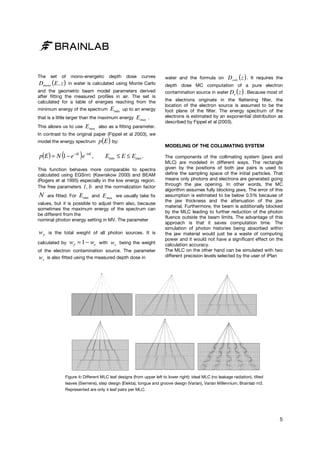
MLC MODEL PRECISION
The MLC model precision can be either “Accuracy
optimized” or “Speed optimized”. “Accuracy optimized”
means, the MLC is modeled with full tongue-andgroove design. It takes into account the air gaps
between neighbor leaves. The “Speed optimized”
option neglects this effect. It employs a model of an
ideal MLC (see section Modeling of the Collimator
System and Figure 4). Therefore this option shortens
the calculation time. The section Modeling of the
Collimator System contains more detailed information
about the MLC modeling.
regular beams and clinical field arrangements in
heterogeneous conditions (conformal beam therapy,
arc therapy and IMRT including simultaneous
integrated boosts). They measured absolute and
relative dose distributions with ion chambers and near
tissue equivalent radiochromic films. The comparison to
calculations has shown that the iPlan MC algorithm
leads to accurate dosimetric results under clinical test
conditions.
Fragoso et al. (2010) performed a dosimetric verification
and clinical evaluation of the MC algorithm in iPlan RT
Dose for application in stereotactic body radiation
therapy (SBRT) treatment planning. They conclude:
“Overall, the iPlan MC algorithm is demonstrated to be
an accurate and efficient dose algorithm, incorporating
robust tools for MC-based SBRT treatment planning in
the routine clinical setting”.
In a similar investigation Petoukhova et. Al. (2010)
presented verification measurements and a clinical
evaluation of the iPlan RT MC dose algorithm for 6 MV
photon energy. They demonstrate that the Monte Carlo
algorithm in iPlan RT “[…] is able to accurately predict
the dose in the presence of inhomogeneities typical for
head and neck and thorax regions with reasonable
calculation times (5–20 min)”.
In a second publication Petoukhova et al. (2011)
performed a dosimetric verification of HybridArc using
an ArcCHECK diode array. The authors conclude that
for different treatment sites, "comparison of the
absolute dose distributions measured and calculated in
iPlan RT Dose with the MC algorithm at the cylindrical
shape of the ArcCHECK diode array for HybridArc
plans gives a good agreement even for the 2% dose
difference and 2 mm distance to agreement criteria."
DISCUSSION
The XVMC code as basis of iPlan Monte Carlo has
been benchmarked by comparison with the “gold
standard” MC algorithms EGSnrc (Kawrakow 2000) and
BEAM (Rogers et al 1995). It has also been validated by
comparison with measurements (see e.g. Fippel et al.
1997, Fippel et al 1999, Fippel et al 2003). A detailed
comparison of XVMC with pencil beam and collapsed
cone algorithms using measurements in an
inhomogeneous lung phantom has been published by
Krieger and Sauer (2005). Dobler et al (2006) have
demonstrated the accuracy of XVMC relative to
conventional dose algorithms using measurements for
extracranial stereotactic radiation therapy of small lung
lesions. An experimental verification of the Monte Carlo
dose calculation module in iPlan RT Dose presented
Künzler et. al. (2009) by testing a variety of single
9

10. REFERENCES
[1]
AAPM Task Group Report No 105: Issues
associated with clinical implementation of Monte Carlobased external beam treatment planning, Medical
Physics 34 (2007) 4818-4853.
Berger M J, Hubbell J H: XCOM: Photon cross
sections on a personal computer, Technical Report
NBSIR 87-3597 (1987) National Institute of Standards
and Technology, Gaithersburg, MD.
[2]
[3]
Berger M J: ESTAR, PSTAR, and ASTAR:
Computer programs for calculating stopping-power and
range tables for electrons, protons, and helium ions,
Technical Report NBSIR 4999 (1993) National Institute
of Standards and Technology, Gaithersburg MD.
[4] Dobler B, Walter C, Knopf A, Fabri D, Loeschel R,
Polednik M, Schneider F, Wenz F, Lohr F: Optimization
of extracranial stereotactic radiation therapy of small
lung lesions using accurate dose calculation algorithms,
Radiation Oncology 1 (2006) 45.
[12] Kawrakow I: Accurate condensed history Monte
Carlo simulation of electron transport. I. EGSnrc, the
new EGS4 version, Medical Physics 27 (2000) 485-498.
[13] Kawrakow I, Fippel M: Investigation of variance
reduction techniques for Monte Carlo photon dose
calculation using XVMC, Physics in Medicine and
Biology 45 (2000) 2163-2183.
[14] Kawrakow I, Fippel M, Friedrich K: 3D Electron
Dose Calculation using a Voxel based Monte Carlo
Algorithm (VMC), Medical Physics 23 (1996) 445-457.
[15] Krieger T, Sauer O A: Monte Carlo- versus pencilbeam-/collapsed-cone-dose calculation in a
heterogeneous multi-layer phantom, Physics in
Medicine and Biology 50 (2005) 859-868.
[16] Künzler T, Fotina I, Stock M, Georg D:
Experimental verification of a commercial Monte Carlobased dose calculation module for high-energy photon
beams, Physics in Medicine and Biology 54 (2009)
7363-7377.
[5]
Fippel M: Fast Monte Carlo dose calculation for
photon beams based on the VMC electron algorithm,
Medical Physics 26 (1999) 1466-1475.
[17] Petoukhova A L, van Wingerden K, Wiggenraad R
G J, van de Vaart P J M, van Egmond J, Franken E M,
van Santvoort J P C: Verification measurements and
Fippel M: Efficient particle transport simulation
through beam modulating devices for Monte Carlo
treatment planning, Medical Physics 31 (2004) 1235-
clinical evaluation of the iPlan RT Monte Carlo dose
algorithm for 6 MV photon energy, Physics in Medicine
1242.
[18] Petoukhova A L, van Egmond J, Eenink M G C,
Wiggenraad R G J, van Santvoort J P C: ArcCHECK
diode array for dosimetric verification of HybridArc,
Physics in Medicine and Biology 56 (2011) accepted for
publication.
[6]
[7] Fippel M, Haryanto F, Dohm O, Nüsslin F, Kriesen
S: A virtual photon energy fluence model for Monte
Carlo dose calculation, Medical Physics 30 (2003) 301311.
[8] Fippel M, Kawrakow I, Friedrich K: Electron beam
dose calculations with the VMC algorithm and the
verification data of the NCI working group, Physics in
Medicine and Biology 42 (1997) 501-520.
[9]
Fippel M, Laub W, Huber B, Nüsslin F:
Experimental investigation of a fast Monte Carlo photon
beam dose calculation algorithm, Physics in Medicine
and Biology 44 (1999) 3039-3054.
and Biology 55 (2010) 4601-4614.
[19] Press W H, Flannery B P, Teukolsky S A,
Vetterling W T: Numerical Recipes in C: The Art of
Scientific Computing, Second Edition, Cambridge
University Press (1992).
[20] Reynaert N, van der Marck S C, Schaart D R, Van
der Zee W, Van Vliet-Vroegindeweij C, Tomsej M,
Jansen J, Heijmen B, Coghe M, De Wagter C: Monte
Carlo treatment planning for photon and electron
beams, Radiation Physics and Chemistry 76 (2007)
[10] Fragoso M, Wen N, Kumar S, Liu D, Ryu S,
Movsas B, Munther A, Chetty I J: Dosimetric verification
643-686.
and clinical evaluation of a new commercially available
Monte Carlo-based dose algorithm for application in
stereotactic body radiation therapy (SBRT) treatment
planning, Physics in Medicine and Biology 55 (2010)
[21] Rogers D W O, Faddegon B A, Ding G X, Ma C M,
We J, Mackie T R: BEAM: A Monte Carlo code to
simulate radiotherapy treatment units, Medical Physics
22 (1995) 503-524.
4445-4464.
[22] Vanderstraeten B, Chin P W, Fix M, Leal M, Mora
G, Reynaert N, Seco J, Soukup M, Spezi E, De Neve W,
Thierens H: Conversion of CT numbers into tissue
[11] ICRU Report No 46: Photon, Electron, Proton and
Neutron Interaction Data for Body Tissues, International
Commission on Radiation Units and Measurements
(1992).
Europe | +49 89 99 1568 0 | de_sales@brainlab.com
North America | +1 800 784 7700 | us_sales@brainlab.com
South America | +55 11 3256 8301 | br_sales@brainlab.com
RT_WP_E_MONTECARLO_AUG11
parameters for Monte Carlo dose calculations: a multicentre study, Physics in Medicine and Biology 52 (2007)
539-562.
Asia Pacific | +852 2417 1881 | hk_sales@brainlab.com
Japan | +81 3 5733 6275 | jp_sales@brainlab.com
10