IMRT

9.17 Intensity-Modulated Radiation Therapy Planning
AL Boyer
J Unkelbach, Harvard Medical School, Boston, MA, USA
ã 2014 Elsevier B.V. All rights reserved.
9.17.1 The Concept of Intensity-Modulated Radiation Therapy 432
9.17.1.1 Prerequisites for the Development of Intensity-Modulated Radiation Therapy 432
9.17.1.2 Rational for IMRT: Concave Target Volumes 432
9.17.1.3 Advantage of IMRT over 3D Conformal Techniques 433
9.17.1.4 Historical Perspective 434
9.17.2 Optimization of Fluence Distributions 435
9.17.2.1 Dose-Deposition Matrix 436
9.17.2.2 IMRT Planning: A Step-by-Step Demonstration 436
9.17.2.2.1 Initialization and input 436
9.17.2.2.2 Formulation as an optimization problem 436
9.17.2.2.3 Solution to the IMRT problem: the optimal treatment plan 437
9.17.2.2.4 Assessing trade-offs 438
9.17.2.3 The IMRT Optimization Problem 438
9.17.2.3.1 Dose-volume effects 439
9.17.2.3.2 Use of clinical outcome models in IMRT optimization 440
9.17.2.3.3 Further remarks 440
9.17.2.4 Optimization Algorithms 440
9.17.2.4.1 Visualization of the FMO problem 441
9.17.2.4.2 Gradient descent 442
9.17.2.4.3 Including second derivatives 443
9.17.3 The Means to Deliver Optimized Fluence Distributions 443
9.17.3.1 SMLC or Step-and-Shoot Delivery 444
9.17.3.1.1 Basic leaf-pair algorithm 445
9.17.3.1.2 Logarithmic direct aperture decomposition 448
9.17.3.1.3 Matrix inversion 449
9.17.3.2 DMLC Delivery 450
9.17.3.2.1 Leaf-pair speed optimization 451
9.17.3.2.2 Special quality assurance 451
9.17.3.3 Dosimetry of the End of the Leaf 453
9.17.3.4 Practical Dosimetry Considerations 456
9.17.4 Direct Aperture Optimization 457
9.17.4.1 Local Leaf Position Optimization 457
9.17.4.1.1 Approximate dose calculation 458
9.17.4.1.2 Optimizing leaf positions 459
9.17.4.2 Aperture Generation Methods 459
9.17.4.2.1 Generating new apertures 459
9.17.4.2.2 Solving the pricing problem 460
9.17.4.3 Extensions 460
9.17.4.3.1 Integration of improved dose calculation 460
9.17.4.3.2 Hybrid methods and extensions 461
9.17.4.3.3 Generalization to constrained optimization 461
9.17.5 Multicriteria Planning Methods 461
9.17.5.1 Prioritized Optimization 461
9.17.5.2 Interactive Pareto-Surface Navigation Methods 462
9.17.5.2.1 Pareto optimality 462
9.17.5.2.2 Navigating the Pareto surface 463
9.17.5.2.3 Approximating the Pareto surface 464
9.17.5.2.4 Remarks 464
Comprehensive Biomedical Physics http://dx.doi.org/10.1016/B978-0-444-53632-7.00914-X 431

9.17.6 Clinical Application of IMRT 465
9.17.6.1 Prostate 465
9.17.6.2 Head and Neck 466
9.17.6.3 Other Sites 466
9.17.6.4 Comparison of IMRT versus 3D-CRT 467
9.17.6.5 Quality Assurance 468
References 469
Glossary
Beamlet/bixel Refers to narrow beam segment of an
incident radiation beam.
Fluence map Refers to the discretized version of the lateral
fluence distribution of an incident radiation beam. The
fluence map specifies the intensity of all beamlets.
Objective function Is a mathematical function to quantify
clinical goals in an IMRT optimization problem.
Pareto surface Refers to the collection of all Pareto-optimal
IMRT treatment plans, that is, plans that cannot be
improved in one objective without worsening at least one
other objective.
9.17.1 The Concept of Intensity-Modulated
Radiation Therapy
The central problem for treating cancer with ionizing radiation
is finding a means to expose malignant cells to a tumoricidal
dose without exposing healthy tissue to a dose that will lead to
unacceptable damage. External beam teletherapy and inter-
nally administered brachytherapy can both be exploited to
this end. The well-known skin-sparing and moderate attenua-
tion properties of megavoltage (4–50 MV) x-rays have led to
their widespread use for treatment of tumors other than skin
cancer by teletherapy. The direction and collimation of the
x-ray beam are to be devised to optimize the dose to the target
tumor while protecting normal structures as much as possible
by collimation. If the tumor dose can be delivered at a suffi-
ciently high level without increasing the dose to normal tissue
to damaging levels, a medically useful probability of control of
tumors can be achieved without producing an unacceptable
risk of damage to normal tissues.
9.17.1.1 Prerequisites for the Development of
Intensity-Modulated Radiation Therapy
There are two technical developments for advanced radiother-
apy treatment planning in the last quarter of the twentieth
century: computerized tomography (CT) and multileaf colli-
mators (MLCs). Three-dimensional tomographic imaging of
the patient using CT and the addition of MLCs to medical
linear accelerators made intensity-modulated radiation ther-
apy (IMRT) technically feasible. Prior to the general access to
CT scanners, teletherapy was planned as treatment fields hav-
ing two-dimensional shapes that could be determined by mea-
suring the anatomy of the patient visible on projection
radiographs. Since these anatomical x-ray shadows were them-
selves projections through the three-dimensional shapes of
the patient’s organs, the locations of invaginations and con-
cave surfaces could not be determined. Even if they could be,
there was no way to cause dose distributions to conform to
these features of three-dimensional target volume surfaces. The
image data sets acquired by CT scanners capable of volume
acquisition are in essence three-dimensional digital models of
patient anatomy, an essential foundation for physical model-
ing of dose delivered by radiotherapy beams. The development
of advanced treatment planning computer systems coupled
with widespread access to fast CT scanners enabled the inves-
tigation of more effective radiotherapy treatment techniques.
These assets led to the development of three-dimensional con-
formal radiotherapy (3D-CRT), techniques that optimize
shaped collimation of multiple fields such that the relatively
uniform dose delivered by each field is confined to the projec-
tion of the target tumor in the direction of each selected x-ray
cone emanating from the treatment machine (Webb, 1993).
Although 3D-CRT is a major improvement on the two-
dimensional treatment planning that preceded it, radiation
oncologists still found that it did not provide the degree con-
trol of the deposition of radiation that they needed.
9.17.1.2 Rational for IMRT: Concave Target Volumes
A classic example occurs with treating the prostate (see Figure 1).
The prostate lies in the midplane of the pelvis beneath the
bladder, between the symphysis pubis and the anterior rectal
wall. The seminal vesicles and often the lateral lobes of the
prostate can form a concave volume into which the convex
anterior wall of the rectum fits. Alternatively, in certain patients,
the rectum can extend around the prostate forming a pocket in
the anterior rectal wall in which the prostate fits. Only millime-
ters of tissue separate the malignant glandular acini in the
interior of the prostate from the radiosensitive lining of the
rectum. The development of tools to plan 3D-CRT treatments
enabled radiation oncologists to visualize the target tumors
relative to isodose surfaces in three dimensions (see Figure 2).
The dilemma that the anatomy of the prostate presents can be
illustrated by the problem faced by radiation oncologists
attempting to utilize 3D-CRT to investigate escalation of dose
to early-stage prostate cancer during the last decade of the twen-
tieth century. It was soon appreciated that in order to realize the
goal of increasing doses to tumor volumes while reducing or
keeping constant doses to the radiosensitive normal rectal wall,
some means were needed to cause the distribution of dose to be
432 Intensity-Modulated Radiation Therapy Planning

shaped around the convex or concave anterior surface of the
rectum. Exploring beam directions and relative intensity
weights, manually optimized by experienced treatment plan-
ners, failed to find a way to avoid overdosing the anterior rectal
wall in order to achieve the high doses to the prostate that the
radiation oncologists were wishing to investigate. Similar situa-
tions abound at other cancer treatment sites. Classical applica-
tions of IMRT include paraspinal tumor geometries and cancers
in the head and neck region. Paraspinal tumors, where the target
volume surrounds the spinal cord that is to be spared from
irradiation, are used to illustrate IMRT planning in
Section 9.17.2.
9.17.1.3 Advantage of IMRT over 3D Conformal Techniques
IMRT refers to radiotherapy delivery methods for which the
fluence distribution in the plane perpendicular to the incident
beam direction is modulated. IMRT can deliver distributions of
dose that flow into concavities and contract from convexities.
Distributions can be made to exhibit diminutions of dose
within the interior of a higher dose volume. Even though
there are limits to the amplitude of these dose modulations,
this feature of IMRT carries a distinct advantage over 3D-CRT in
most instances. The capability of avoiding delivering full doses
to uninvolved sensitive structures (organs at risk or OARs) near
target volumes requiring high doses is arguably the major
advantage of IMRT. Radiation oncologists were quick to inves-
tigate and exploit IMRT for the treatment of cancer of the
prostate. Figure 3 illustrates the advantage of IMRT over 3D-
CRT in a prostate treatment site. The dose delivered by IMRT to
the convex anterior rectal and to the base of the bladder can be
controlled to the extent that the dose to the prostate can be
raised to levels that would risk perforations of the rectal wall if
attempted with 3D-CRT.
Since OARs can be made to receive few doses with IMRT than
with 3D-CRT, it is possible to increase the dose per daily fraction
with IMRT. This ‘accelerated’ pace of dose delivery leads to a
greater probability of tumor cell kill. Modest increases in dose
per fraction can produce benefits worth exploiting.
A secondary advantage is the automated nature of the plan-
ning process with IMRT. A highly experienced planner may be
able to devise complex treatment field arrangements (employ-
ing field-in-field techniques and selecting unique beam angles)
that compete with IMRT plans. But time and training efforts are
required to produce such mastery. There are few opportunities
for quantifying the production of such plans, and the vagaries of
an artistic skill lead to inconsistent results. The IMRT process
lends itself the use of mathematical optimization techniques,
which automate and optimize the design of incident radiation
beams and thereby consistently produce plans of high quality.
B
P
R
95% isodose
Figure 2 Three-dimensional conformal radiotherapy (3D-CRT)
visualization of anatomical structures relative to isodose surface for a
prostate treatment plan. The bladder (B in blue) and the rectum (R in
green) are visualized using a wire-frame rendering. The prostate (P in red)
and seminal vesicles (S in white) are rendered as solid surfaces. The
pose is similar to Figure 1. A wire frame covers the surface corresponding
to a dose that is 95% as great as the maximum dose within the
volume. The treatment strategy was composed of four large fields to treat
involved lymph nodes followed by smaller fields to treat the prostate
alone. The posterior 95% isodose surface penetrates into the anterior wall
of the rectum.
Figure 1 A sagittal section through the male pelvis illustrating the close
proximity of the prostate (P) to the bladder (B) and the rectum (R).
The anterior rectal wall is covered in the lateral projection by the lateral
lobes of the prostate and the seminal vesicles.
Intensity-Modulated Radiation Therapy Planning 433

9.17.1.4 Historical Perspective
The development of IMRT occurred over the last decade of the
twentieth century and the first decade of the twenty-first cen-
tury (Bortfeld, 2006; Webb, 2003). As with most successful
modern technologies, after its initial development, additional
refinements and improvements have continued up to the pre-
sent. IMRT was developed by an international collection of
medical physicists from many radiation oncology centers.
Anders Brahme shared his early thoughts on the subject
through publications and symposia (Brahme et al., 1982;
Lind and Brahme, 1985), an example being the Workshop on
Developments in Dose Planning and Treatment Optimization
at the Karolinska Institute in Stockholm, Sweden, in 1991.
Ideas and information were exchanged through formal pre-
sentations and informal face-to-face discussions at the annual
meetings of the major medial physics and radiation oncology
professional societies, such as the European Society for Radi-
otherapy & Oncology (ESTRO), the American Society for
Radiation Oncology (ASTRO), and the American Association
of Physicists in Medicine (AAPM), and through their associa-
tion journals. The willingness of individual investigators to
share their work candidly with their colleagues, to exchange
criticisms, and to maintain friendly rivalries was the driving
force contributing to the rapid growth and sophistication of
the technology. The British government support of the Royal
Marsden Hospital Joint Department of Physics and Institute of
Cancer Research in Sutton, Surrey, United Kingdom
(Webb, Convery, and Rosenbloom); the German support of
the Deutsches Krebsforschungszentrum (DKFZ) in Heidelberg,
Germany (Schlegel, Bortfeld, and Stein); and the support of
multiple investigators in the United States by the National
Cancer Institute (NCI) poured millions of dollars into the
effort. Leaders of commercial entities (notably Varian, Sie-
mens, Elekta, and the NOMOS Corporation) had the foresight
to invest substantial commercial funding, including grants to
academic investigators, into the development of the MLC hard-
ware and IMRT treatment planning software. These webs of
relationships make it difficult to lay out a single linear chro-
nology of the development of ideas and key demonstrations of
the technology.
The history of NCI grant RO1-CA43840 (Arthur Boyer, PI)
can be used as an example. The application was written in
September and submitted to the NCI by the MD Anderson
Cancer Center (MDACC) in Houston, TX, in October 1991. It
was awarded for 5 years with a start date of 1 July 1992. The
three research objectives were to explore the development of
three tools:
1. Conformal optimization tools. Optimal fluence distributions
for beams from fixed directions were to be developed as had
been proposed in the inverse planning work of Brahme
(1988a,b). Dose-volume histograms were to be used as a
means of control and evaluation of the optimization. Opti-
mization using simulated annealing, as had been investi-
gated by Webb (1989), was to be compared with ‘beam
ensemble’ optimization proposed by Brahme (Ka¨llman
et al., 1988), and techniques were to be borrowed from
CT reconstruction (Bortfeld et al., 1990). The work by
Censor et al. (1988) was referenced. A biological objec-
tive function was to be considered as an alternative.
Section 9.17.2 reviews the foundations of optimizing flu-
ence distributions.
2. Dynamic MLC (DMLC) compensation tools. A sequence of
radiation exposures made with stationary leaf positions was
to be developed to deliver the fluence distributions com-
puted using the first tool (see Section 9.17.3). Film dosim-
etry was to be employed to verify the delivery of the dose
distributions. The proposal for MLC delivery referenced the
earlier work by Brahme (Lind and Brahme, 1987).
IMRT
B B
P P
R R
3D-CRT
Figure 3 Rendering of relative dose by color on the surfaces of the bladder (B), prostate (P), and rectum (R) viewed from the patients’ right side while the
patient is lying on their back. Anterior is toward the top of the figures and posterior is toward the bottom. Shades of red on the bladder and rectum
indicate increasing levels of dose. The right image is rendered from a 3D-CRT plan. The image on the left is rendered from an intensity-modulated
radiotherapy (IMRT) plan for the same patient. In both cases, the uniform red coloring of the prostate surface demonstrates that the target would be uniformly
treated. The reduction in red in the IMRT rendering on the anterior rectal wall and the inferior surface of the bladder compared with the 3D-CRT rendering
demonstrates the calculated reduction of dose to these organs at risk (OAR) using IMRT. Figure reprinted with permission from Varian Medical Systems.

3. Electronic Portal Imaging Device (EPID) field verification tools.
Patient position and the MLC treatment sequences were to
be verified using EPID images. Correlations of image fea-
tures were to use Fourier transform-based correlation.
Clearly, these concepts had not been developed in a vacuum.
The proposal wove together threads of existing ideas along with a
few innovations into a yarn that strung together the whole treat-
ment planning, delivery, and verification process. The reviewers
were convinced by the preliminary data in the application that
the investigative team could carry the project through. The arrival
of Thomas Bortfield at the MDACC in 1992 within weeks of the
beginning of the project, as a postdoctoral fellow, contributed
inestimably to the early success of the effort. Within 9 months, a
three-dimensional inverse planning algorithm had been derived
from his earlier thesis work in two dimensions, the step-and-
shoot sweeping window algorithm had been refined and dem-
onstrated with a clinical MLC newly installed at the MDACC
(Bortfeld et al., 1994), and dose distributions had been delivered
to a film phantom that proved the feasibility of producing three-
dimensional dose volumes bounded by concave surfaces
(Bortfeld et al., 1994). An agreement was brokered with Clif
Ling, the chair of the physics department, and Rodhe Mohan,
the chief of the excellent software development group at the
Memorial Sloan Kettering Cancer Center (MSKCC), that Bortfeld
would tarry in New York in mid-1993 on his way back to
Germany long enough to share the software that had been devel-
oped in Houston. The MSKCC group delivered the first clinical
IMRT treatment using this form of the technology to a prostate
cancer patient (Ling et al., 1996) in 1995. The same year (1995),
the grant was transferred from MDACC to Stanford University
where the PI had accepted an appointment as the director of the
Radiation Physics Division of the Department of Radiation
Oncology. The division was collaborating with the Department
of Neurosurgery at Stanford to develop the Cyberknife Robotic
Radiosurgery System and had just recently treated the first patient
with this device. Soon, postdoctoral fellows and staff funded by
the grant were working on both robotic and cone-beam delivery.
The cone-beam IMRT development was advanced by collabora-
tion with the NOMOS Corporation. Bruce Curran had moved
from academia to industry to work on the implementation of a
cone-beam optimizer and MLC sequence composer within the
NOMOS planning system. Curran installed a prototype treat-
ment planning system at Stanford in 1996 with the able assis-
tance of Stanford faculty physicist Lei Xing (Xing et al., 1999).
The first patient to receive IMRT treatments with the cone-beam
approach using commercial assets received their initial treatment
at Stanford on 11 November 1997. The procedure required
12 min. That the audacious objectives of the grant would be
realized to the extent that patients would be treated by the end
of the last year of the award can only be attributed to the industry
and ingenuity of the medical physicists directly and indirectly
involved. This example demonstrates how medical physicists
from the DKFZ, MSKCC, MDACC, and Stanford worked together
without institutionally initiated formal prearrangements, shared
information and critical software, carried out key clinical devel-
opments, and worked with industry to make IMRT a viable
medical tool. But this example is only a few strands of the global
web of medical physicists who made invaluable contributions.
The list of the many other physicists working on IMRT and their
accomplishments could fill the rest of this chapter. At the risk of
seeming to overlook these worthies, the reader is referred to more
extensive historical discussions (Webb, 2001).
9.17.2 Optimization of Fluence Distributions
IMRT refers to radiotherapy delivery methods for which the
fluence distribution in the plane perpendicular to the incident
beam direction is modulated. To that end, we assume that the
radiation beam is divided into small beam segments, which are
in principle deliverable by a MLC. The lateral fluence distribu-
tion of the beam is thereby discretized into small elements,
which are commonly referred to as beamlets or bixels (see
Figures 4 and 5 for an illustration). A beamlet is a pyramidal
Figure 4 An opposed pair of multileaf collimator (MLC) leaves (gray)
are driven by electric motors. Their positions are encoded as well. They
form a gap between their ends within which an integer number of
beamlets (yellow) is delivered along their motion path (blue). The length
of the beamlet in the direction of leaf travel is a parameter selectable
for the treatment planning system. The width of the beamlet
(perpendicular to leaf motion) is determined by the leaf width. Note the
curved leaf ends and the tongues and grooves on the sides of the leaves.
Voxel i
Bixel j
Figure 5 Schematic illustration of the beamlet and dose-deposition
matrix concepts in IMRT. The incident radiation beam is divided
into beamlets; the dose-deposition matrix stores the dose contribution of
each beamlet to each voxel in the patient.

radiation cone whose apex is at the center of the x-ray source
(bremsstrahlung x-ray target) and whose base is a rectangle
(see Section 9.17.3.1 for details). For an MLC with 1 cm leaf
width, the fluence distribution is represented by the intensities
of 1Â1 cm beamlets. Nowadays, modern MLCs with a smaller
leaf width often allow for a finer discretization into 5Â5 mm
beamlets. The discrete representation of the fluence is com-
monly referred to as the fluence map.
In this section, we discuss the concepts and methods to
determine the intensity of each beamlet. This problem is referred
to as the fluence map optimization (FMO) problem. To that
end, we first introduce the concept of the dose-deposition
matrix, which relates the beamlet intensities to the dose distri-
bution in the patient (Section 9.17.2.1). In Section 9.17.2.2,
the concept of IMRT planning will be demonstrated step by step,
using a paraspinal tumor case as an example. The goal of FMO is
to determine the beamlet intensities in such a way that the
chance of tumor cure is maximized, while the probability of
severe normal tissue complications is minimized. We will see
how this notion is translated into mathematical terms by
formulating IMRT planning as a mathematical optimization
problem (Section 9.17.2.3). Section 9.17.2.4 will provide an
introduction to the most basic optimization algorithms that
can be used to solve FMO problems.
9.17.2.1 Dose-Deposition Matrix
The quality of a treatment plan is primarily judged based on
the dose distribution in the patients. Thus, we would like to
determine the fluence maps of the incident beams as to best
approximate a desired dose distribution. In order to achieve
this, we have to relate the fluence to the dose distribution in the
patient. In this section, we introduce the dose-deposition
matrix concept, which provides exactly this link.
For IMRT planning, the patient is discretized into small
volume elements referred to as voxels. We assume that the
dose-calculation algorithm can provide the dose distribution
of any incident beam. Therefore, the dose-calculation algo-
rithm can be used to obtain the dose distribution in the patient
for every beamlet in the fluence map. Let us denote the dose
that beamlet j contributes to voxel i in the patient for unit
intensity as Dij; and let us denote the intensity of beamlet j as
xj. The total dose di delivered to voxel i is then simply given by
the superposition of all beamlet contributions:
di ¼
X
j
Dijxj
Here, the matrix of dose contributions Dij of beamlets j to
voxel i is referred to as the dose-influence matrix or the dose-
deposition coefficients. The dose-deposition matrix concept is
illustrated in Figure 5. In practice, the fluence is commonly
quantified in monitor units (MU). In this case, the natural unit
of the dose-deposition matrix is Gy/MU, such that the resulting
dose distribution in the patient is obtained in Gy. The dose-
deposition matrix concept is convenient since it allows for a
separation of the mathematical optimization of beamlet inten-
sities xj from the dose-calculation algorithm: in IMRT plan-
ning, the dose-deposition matrix is often calculated up front
and held in memory. Subsequently, the dose distribution is
obtained by a simple matrix multiplication d¼Dx.
9.17.2.2 IMRT Planning: A Step-by-Step Demonstration
In this section, we demonstrate the concepts of IMRT planning
for an example case. We consider the patient shown in Figure 6.
In this case, the target volume to be treated with radiation (red
contour) surrounds the spinal cord (green contour). The latter
is the main dose-limiting organ at risk, which is to be spared
from irradiation. In addition, the kidneys (orange contours)
are located in proximity to the target volume, representing the
secondary OAR to be spared.
9.17.2.2.1 Initialization and input
For IMRT planning, a segmentation of the patient is required,
which specifies to which organ or anatomical structure each
voxel belongs to. In the example in Figure 6, each voxel is
assigned to the spinal cord, the target volume, the kidneys, or
the remaining healthy tissues in the patient. In addition, we
require a setup of the fluence map. Similar to 3D-CRT, this
starts with selecting the location of the isocenter. For IMRT
planning, we determine the set of all beamlets that are poten-
tially helpful in finding the most desirable treatment plan.
Loosely speaking, this corresponds to all beamlets that con-
tribute a significant dose to the target volume. A common
method for initializing the fluence map consists in including
all beamlets for which the central axis of the corresponding
beam segment intersects the target volume. Given the voxel
discretization of the patient, the isocenter, and the beamlet grid
for each incident beam, a dose-calculation algorithm is used to
calculate the dose distribution of each beamlet in the patient,
that is, the dose-deposition matrix, Di j.
9.17.2.2.2 Formulation as an optimization problem
In order to determine the optimal incident fluence distribu-
tions, we have to specify the desired dose distribution. In other
words, we have to characterize what a ‘good’ treatment plan is.
In the example case in Figure 6, treatment planning aims at
different goals:
1. Deliver a prescribed dose dpres
to the target volume. As in
most cases, the target volume contains tumor cells
Figure 6 A typical indication for IMRT: a paraspinal tumor geometry.
The tumor (red) entirely surrounds the spinal cord, which is to be
spared from irradiation. In addition, the kidneys are located in proximity
to the target volume.

embedded in a normal tissue stroma such that treatment
planning aims at a homogeneous dose in the target, avoid-
ing both underdosing, which would fail to kill all the tumor
cells, and overdosing, which would destroy the normal
tissue stroma along with blood vessels and nerves passing
through it. If enough of the stroma survives, tissue will
regrow in the target volume. Otherwise, the target volume
will contain an abscess leading to muscle, nerve, and circu-
lation problems.
2. Minimize dose to the kidneys.
3. Aim at a conformal dose distribution and avoid unneces-
sary dose to all healthy tissues.
4. Limit the dose to the spinal cord. The maximum dose
delivered to any part of the spinal cord has to stay below a
maximum tolerance dose dS
max
.
For IMRT planning, these goals have to be translated into
mathematical terms. This is done by defining functions, which
represent measures for how good a treatment plan is and
whether it is acceptable at all. In this context, we distinguish
objectives and constraints:
Constraints are conditions that are to be satisfied in any case.
Every treatment plan that does not satisfy the constraints
would be unacceptable. The set of constraints together
defines the feasible region, which corresponds to the set
of treatment plans that satisfy all constraints.
Objectives are functions that measure the quality of a treatment
plan. They may represent measures to quantify how close a
treatment plan is to the ideal or desired treatment plan.
In the previously mentioned example, the first three goals
can be formulated as objectives; the fourth goal of enforcing a
strict maximum on the spinal cord dose represents a constraint.
The goal of delivering a homogeneous dose to the target vol-
ume can be formulated via a quadratic objective function:
fT dð Þ ¼
1
NT
XNT
i¼1
di À dpres
ð Þ2
where the summation occurs over the NT voxels located by
three-dimensional indices i that belong to the target volume.
Ideally, every voxel that belongs to the target volume receives
the prescribed dose dpres
, which corresponds to a value of zero
for the function fT. Otherwise, fT yields the average quadratic
deviation from the prescribed dose. The larger the objective
value is, the more the dose deviates from the prescription dose,
corresponding to a worse treatment plan.
Similarly, the goal of minimizing the dose to the kidneys
can be formulated as an objective function. For example, we
can define the objective fK as
fK dð Þ ¼
1
NK
XNK
i¼1
di
that aims at minimizing the mean dose to the kidneys. The goal
of conforming the dose distribution to the target volume can,
for example, be described via a piecewise quadratic penalty
function
fH dð Þ ¼
1
NH
XNH
i¼1
di À dmax
i
À Á2
þ
where the þ operator is defined through (di Àdi
max
)þ ¼di Àdi
max
if di !di
max
and zero otherwise. Thus, di
max
is the maximum dose
that is accepted in voxel i; dose values exceeding di
max
are penal-
ized quadratically. Clearly, in normal tissue voxels directly adja-
cent to the target volume, high doses are unavoidable, whereas at
large distance from the target volume, treatment planning
should aim at avoiding unnecessary dose. Therefore, di
max
can
be chosen based on the distance between voxel i and the target
volume.
Finally, we would like to ensure that the dose in all voxels
that belong to the spinal cord does not exceed a maximum
tolerance dose dS
max
. If we will not accept any treatment plan
that exceeds the maximum dose, this can be implemented as a
constraint, not an objective. In this case, we can formulate the
constraint as
di dmax
S for all i E S
where S is the set of indices of three-dimensional vectors
pointing to voxels within the spinal cord volume.
Treatment planning simultaneously aims at minimizing all
of the previously mentioned objective functions, that is,
ideally, we would like each tumor voxel to receive the pre-
scribed dose, while no dose is delivered to the normal tissues.
It is clear that the objectives associated with different structures
are inherently conflicting. Thus, the treatment planner will
have to weight these conflicting objectives relative to each
other and accept a compromise. The traditional approach in
IMRT planning consists in manually assigning importance
weights w to each objective, using a high weight for the most
important objective and a smaller weight for less important
goals. The best treatment plan is then defined as the one that
minimizes the weighed sum of objectives:
wTfT dð Þ þ wKfK dð Þ þ wHfH dð Þ
Given the mathematical formulation of the clinical goals,
IMRT planning uses mathematical optimization algorithms in
order to determine the fluence map x, corresponding to the
dose distribution d¼Dx, which minimizes the weighted sum
of objectives, subject to all constraints of the dose distribution
and under the condition that all beamlet weights have to be
positive. We will further discuss optimization algorithms in
Section 9.17.2.4. In the succeeding text, we first take a look
at the result of such an optimization.
9.17.2.2.3 Solution to the IMRT problem: the optimal
treatment plan
Figure 7 shows the optimal dose distribution obtained for a
specific choice of optimization parameters: the spinal cord
dose was constrained to two-third of the prescription dose.
The voxel-dependent maximum dose di
max
in the conformity
objective was formulated to provide a dose falloff to one-third
of the prescription dose at 1 cm distance from the target sur-
face. Nine equispaced coplanar incident beams are used. It is
apparent that IMRT is capable of conforming the high-dose
region relatively tightly to the target volume. In particular, the
dose to the spinal cord can be reduced to doses much below
the prescription dose. This would not be possible using 3D
conformal techniques without the possibility of modulating
the intensity of the incident radiation beams.

Figure 8 shows the dose contribution of two out of nine
beam directions, illustrating the use of intensity modulation.
The intensities of the beamlets that intersect with the spinal
cord are reduced to near zero. This allows for a dose reduction
in the spinal cord but at the same time yields an inhomoge-
neous dose distribution in the target volume. All nine beams in
combination deliver the prescribed, homogeneous dose distri-
bution to the target volume.
9.17.2.2.4 Assessing trade-offs
Different objectives in IMRT planning are inherently conflict-
ing. Clearly, there is a trade-off between delivering dose to the
tumor and reducing dose to healthy tissues. In the previously
mentioned example, the dose to the spinal cord is constrained
to two-third of the prescription dose, which compromises the
coverage of the target volume. In regions near the spinal cord,
the target volume does not receive the prescribed dose. To
improve the coverage of the target volume, higher doses to
the spinal cord have to be accepted. In addition, IMRT plan-
ning involves trading off the dose burden of adjacent healthy
tissues. In the previously mentioned example, there is a trade-
off between sparing the kidneys from irradiation and the con-
formity of the dose distribution in the remaining normal
tissue. Achieving a very low dose in the kidneys leads to higher
doses in the normal tissue anterior and posterior to the target
volume. This is illustrated in Figure 9. In comparison with
Figure 9, the weighting factor for the kidney mean dose was
increased and the weighting factor for the conformity objective
was decreased. Thereby, the kidney dose could be substantially
reduced. Through the use of mathematical optimization, the
beam segments that penetrate the kidneys are automatically
avoided. However, this comes at the price of a less conformal
dose distribution, that is, higher doses in the normal tissue
anterior and posterior to the target volume.
In today’s clinical practice, the treatment planner chooses
the objective weights manually, based on prior experience and
trail-and-error experience with the treatment plan before them.
In Section 9.17.5, we discuss multicriteria optimization
methods that represent a more elaborate approach to control-
ling the trade-off between different objectives.
9.17.2.3 The IMRT Optimization Problem
In the previous section (Section 9.17.2.2), we illustrated IMRT
planning step by step for an example case. In this section, we
take a more formal look at IMRT planning as a mathematical
Figure 8 The contribution of two of nine beam directions. The beam in panel (a) directly from the posterior demonstrates the symmetric reduction of
intensity of the beamlets that intersect the spinal cord but not the kidney. One side of the posterior oblique beam in panel (b) intersects part of the
kidney and is less intense than the opposite side of the beam that does not intersect a kidney.
Figure 7 IMRT dose distribution for the paraspinal case example,
demonstrating the ability of IMRT to conform the dose distribution to
concave target volumes.
Figure 9 IMRT dose distribution for the paraspinal case example,
demonstrating the trade-off between conformity of the dose distribution
and the minimization of the kidney dose.

optimization problem. Mathematically, the FMO problem can
be formulated as
minimize
x
f dð Þ
subject to gk dð Þ ck
di ¼
X
j
Dijxj xj ! 0
The first line indicates that we minimize an objective func-
tion f with respect to the fluence map x, which corresponds to
dose distribution d. The second line indicates that we are
restricted to dose distributions that satisfy the constraints
gk(d) ck. The third line specifies the relation between fluence
and dose, and the last line requests that all beamlet intensities
have to be positive in order to be physically meaningful. Treat-
ment planning involves balancing different clinical objectives.
Therefore, the objective function f is a weighted sum of indi-
vidual objectives:
f dð Þ ¼
X
n
wnfn dð Þ
Here, wn are positive weighting factors that are used to
control the relative importance of different terms in the com-
posite objective function.
The objective function that may be the most commonly
used in current treatment planning systems is a piecewise
quadratic penalty function:
fn dð Þ ¼
1
Nn
XNn
i¼1
di À dmax
i
À Á2
þ
or fn dð Þ ¼
1
Nn
XNn
i¼1
dmin
i À di
À Á2
þ
Here, dmax
is a maximum tolerance dose for an organ,
which is usually specified by the treatment planner through
the graphical user interface in the treatment planning system.
Similarly, for target volumes, dmin
is a minimum dose that is to
be delivered to the target volume. Common constraints are
maximum dose values in OAR and minimum doses in target
volumes. In the next subsection, additional commonly used
objectives and constraints are discussed.
9.17.2.3.1 Dose-volume effects
An organ at risk will typically receive an inhomogeneous dose
distribution. Often, the question arises whether it is preferable
to irradiate a small part of the organ to a large dose while
sparing the remaining parts to a large extent or whether it is
better to spread out the dose and avoid large doses in all parts
of the organ. In that context, one distinguishes parallel organs
and serial organs. For organs with a serial structure, the func-
tion of the whole organ will fail if one part of the organ is
damaged. One prominent example for a serial organ is the
spinal cord. For serial organs, it is therefore crucial to limit
the maximum dose delivered to the organ, rather than the
mean dose. For a parallel organ, the function of the organ as
a whole is preserved even if a part of the organ is damaged. An
example for a parallel organ is the lung. The dependence of a
clinical outcome on the irradiated volume of an organ is com-
monly referred to as a volume effect or dose-volume effect. For
IMRT planning, clinical knowledge on dose-volume effects is
to be translated into appropriate objective functions. Today,
mainly two types of objective/constraint function are being
applied: Dose-Volume Histogram (DVH) objectives and the
concept of equivalent uniform dose (EUD).
9.17.2.3.1.1 DVH objectives and constraints
The clinical evaluation of treatment plans often uses the dose-
volume histogram. A typical evaluation criterion for the target
volume is that at least 95% of the target volume should receive
a dose equal or higher than the prescription dose. Similarly, a
criterion for an OAR could be that at most 20% of the organ
should receive more than 30 Gy.
From an optimization perspective, it is not straightforward
to handle DVH constraints in a rigorous way. A naive imple-
mentation of a DVH constraint requires the use of integer
variables. For example, the constraint that no more than v%
of an organ should receive a dose higher than dcrit
can formally
be written as
1
N
XN
i¼1
bi v
bi ! M di À dcrit
À Á
bi E 0; 1f g
where M is a large constant. Here, bi is a binary integer variable
that is introduced for every voxel, which takes the value 1 if the
dose di exceeds dcrit
and 0 if di is smaller than dcrit
. The use of
integer variables represents a different type of optimization
problem, is computationally demanding, and requires algo-
rithms that differ considerably from those that is described in
Section 9.17.2.4.
In practice, DVH constraints are therefore handled approx-
imately through a heuristic tactic. Given the current dose dis-
tribution, one can identify the fraction of voxels that exceed the
dose level dcrit
. If this fraction is smaller than v, the DVH
constraint is fulfilled. Otherwise, a quadratic penalty function
is introduced that aims at reducing the dose to those voxels that
exceed dcrit
by the least amount, neglecting the fraction v that
receives the highest dose.
9.17.2.3.1.2 Equivalent uniform dose
An alternative approach to quantifying dose-volume effects
consists in using generalized mean values of the dose distribu-
tion defined as
EUD dð Þ ¼
1
N
XN
i¼1
dið Þa
" #1=a
for Ni & OAR
where the exponent a is larger than one for OARs. For the special
case a¼1, EUD(d) is equivalent to the mean dose in the organ.
In the limit of large a values, the value of EUD(d) approaches
the maximum dose in the organ. Thus, parallel organs are
described via a small value of a close to 1, whereas serial organs
are described via large values of a: (approximately 10). The
generalized mean value is commonly referred to as EUD.
The generalized mean value can also be applied to target
volumes by using negative exponents. For a large negative
value of a, the EUD approaches the minimum dose in the
target volume. In practice, exponents in the range of a¼À10
toÀ20 are considered.

9.17.2.3.2 Use of clinical outcome models in IMRT
optimization
From the beginning of the development of IMRT, the question
regarding the adequate objective function to be used has per-
sisted. Intuitively, we would like to translate the notion of
‘maximizing the tumor control probability (TCP)’ while
‘minimizing the normal tissue complication probability
(NTCP)’ more directly into mathematical terms (Brahme
et al., 1988; Ka¨llman et al., 1992).
9.17.2.3.2.1 Sigmoid outcome models
One of the most common methods for relating treatment out-
come to the dose distribution consists in performing logistic
regression. As an example, we consider NTCP models. However,
the same methodology can be applied to TCP models. The
severity of a radiation side effect is clinically assessed in discrete
stages. Typically, one is interested in avoiding severe complica-
tions. For example, in the treatment of lung cancer, treatment
planning may aim at minimizing the probability for radiation
pneumonitis of grade two or higher. This converts the observed
clinical outcome into a binary outcome label. NTCP modeling
can thus be considered as a classification problem, which aims
at estimating the probability of a complication given features of
the dose distribution. Standard statistical classification methods,
such as logistic regression, can be applied to this problem. In
logistic regression, the NTCP model is given by
NTCP dð Þ ¼
1
1 þ exp Àf d; qð Þð Þ
Here, f is a function of the dose distribution d and the
model parameters q. The central problem in statistical analysis
and modeling of patient outcome consists in determining the
function f, that is, selecting features of the dose distribution
that are correlated with outcome. One of the most commonly
used representations of f is given by
NTCP dð Þ ¼
1
1 þ exp g TD50 À EUD dð Þð Þ½ Š
In this case, f is a linear function of a single feature of the
dose distribution, namely, the EUD. For EUD(d)¼TD50, the
value of NTCP evaluates to 0.5, that is, TD50 corresponds to
the effective dose that leads to a complication probability of
50%. The parameter g determines the slope of the dose–
response relation. The NTCP model has three parameters
(TD50, g, and the EUD exponent a) that can be fitted to outc-
ome data, for example, through maximum likelihood
methods. This NTCP model is equivalent to the Lyman–
Kutcher–Burman (LKB) model, except that the LKB model
traditionally uses a different functional form of the sigmoid.
Although phenomenological outcome models may play an
increasing role in treatment plan evaluation, their capabilities
from a treatment plan optimization perspective have remained
limited so far. The previously mentioned NTCP model represents
an increasing function of the EUD, that is, higher EUD always
leads to higher NTCP, independent of the parameters TD50 and
g. As a consequence, the dose distribution that minimizes EUD is
the same as the dose distribution that minimizes NTCP. Hence,
from an IMRT optimization perspective, minimizing EUD and
NTCP is equivalent (Romeijn et al., 2004).
9.17.2.3.3 Further remarks
9.17.2.3.3.1 Linear programming formulations
One of the fundamentals of FMO is the linear relation between
the dose and the incident fluence. Due to the linearity, it is
possible to formulate IMRT planning as a linear optimization
problem (LP). LPs are optimization problems for which both
the objective f and all constraint functions gk are linear func-
tions of the optimization variables. At first glance, an exclusive
use of linear functions appears restrictive. However, it turns out
that most nonlinear objective functions currently can be mim-
icked using linear formulations by introducing auxiliary opti-
mization variables. LP formulations for FMO have mostly been
studied in research environments. However, the first-generation
IMRT planning systems and contemporary commercial planning
systems are primarily focused around quadratic objective func-
tions and DVH- and EUD-based objective and constraint
functions.
9.17.2.3.3.2 Size of the optimization problem
IMRT treatment planning corresponds to a large-scale optimi-
zation problem since it involves a large number of variables.
The number of beamlets for a single incident beam depends on
the size of the target volume and the beamlet resolution (typ-
ically 5 or 10 mm) and is usually in the order of 102
–103
for
each beam direction. Assuming that ten beam directions are
used, the total number of beamlets is expected to be in the
order of 103
–104
. Furthermore, the patient is discretized into
voxels, with a typical resolution of 2–4 mm, resulting in the
total number of voxels in the order of 106
.
If all beamlets contributed a significant dose to all voxels in
the patient, the number of elements in the dose-deposition
matrix would be 109
–1010
. If each element is stored as a 4-
byte integer, the dose-deposition matrix requires approximately
10 GB of memory. However, in practice, the dose contributions
to voxels at large distance from a beamlet’s central axis are set
to zero. Thereby, the total number of nonzero elements is
substantially reduced, and the dose-deposition matrix can be
stored in a sparse format.
9.17.2.3.3.3 Convexity
Many objective functions commonly applied in IMRT plan-
ning are convex. This is in particular the case for the piecewise
quadratic objective, the linear objectives, and the generalized
EUD for exponents |a|>1. The convexity property of objective
and constraint functions has important implications for the
optimization of fluence maps. An optimization problem
defined through a convex objective function f and convex
constraint function gk has a unique global minimum, that is,
there are no local minima, which are not the global minimum.
Thus, gradient descent-based optimization algorithms as
described in Section 9.17.2.4 will reliably find the optimal
fluence map. The only nonconvex functions commonly
applied in practice are DVH constraints.
9.17.2.4 Optimization Algorithms
Our goal in this chapter is to provide the reader with an
understanding of the most basic optimization algorithms that
do not require advanced knowledge of optimization theory. In

Section 9.17.2.4.1, we start with a geometric visualization
of the IMRT optimization problem. In Section 9.17.2.4.2, the
gradient descent algorithm in the context of IMRT is described,
which in principle is sufficient to optimize fluence maps. In
Section 9.17.2.4.3, extensions of gradient descent methods
toward quasi-Newton algorithms are outlined. Certainly, the
field of IMRT optimization has advanced significantly, and
increasingly complex algorithms for constrained optimization
are being applied. These algorithms require knowledge of opti-
mization theory, which is beyond the scope of this chapter. The
interested reader is referred to the optimization literature (e.g.,
Bertsekas, 1999 or Nocedal and Wright, 2006) or a review of
mathematical optimization problems in radiotherapy by
Ehrgott et al. (2010).
9.17.2.4.1 Visualization of the FMO problem
Due to the large number of beamlets (optimization variables),
it is not possible to visualize directly the objective and con-
straint functions for a full IMRT planning problem. Neverthe-
less, it is helpful to understand the structure of the IMRT
optimization problem. To that end, we consider a simplified
version of an IMRT planning problem in which only two
beamlets and four voxels are considered. We consider the
following dose-deposition matrix:
D ¼
1:3 0:7 0:1 1:0
0:7 1:3 0:5 0:3

where the first two columns correspond to the tumor voxels
and columns 3 and 4 correspond to OAR voxels. We further
assume that we aim to deliver a dose of 2 to both of the tumor
voxels, and we impose a maximum dose constraint of 0.8 and
1.0 on the OAR voxels.
The goal of delivering the prescribed dose to the tumor
voxels is expressed via a quadratic objective function. The
optimization for this illustrative example can be formulated as
minimize
1
2
X2
i¼1
di À 2ð Þ2
subject to d3 0:8
d4 1:0
di ¼
X2
j¼1
Dij xj xj ! 0
Since we only have two optimization variables, the objec-
tive and constraint functions can be visualized explicitly. This
is done in Figure 10. The objective function is depicted via
isolines. Since we consider a quadratic objective function, it
represents a two-dimensional parabola. The minimum of the
objective function is located at beamlet intensities x1 ¼1 and
x2 ¼1. At this point, both tumor voxels receive the prescribed
dose and the objective function is zero.
We now consider the constraints on the OAR voxels. Since
the dose in each voxel is a linear function of the beamlet
intensities, the constraints represent hyperplanes in beamlet
intensity space, that is, lines in two dimensions. In Figure 10,
we show the lines where the constraints d3 ¼0.8 and d4 ¼1.0
are met exactly. For all beamlet intensities beyond these lines,
the maximum dose to an OAR voxel is exceeded. All beamlet
intensity combinations below the lines form the feasible
region. Thus, the optimal solution to the IMRT planning prob-
lem is given by the point within the feasible region that has the
smallest value of the objective function. In this example, this is
approximately given by x1 ¼0.7 and x2 ¼1.2 and is indicated
by the red dot in Figure 10. By multiplying this solution with
the dose-deposition matrix, we obtain the corresponding opti-
mal dose distribution.
In this case, the constraint for OAR voxel 4 is binding, that
is, the OAR voxel receives the maximum dose we allow for. We
further note that the minimum of the objective function is
outside of the feasible region, which means that, in order to
fulfill the maximum OAR dose constraint, we have to compro-
mise in terms of target dose homogeneity.
9.17.2.4.1.1 Approximate handling of constraints through penalty
functions
A common approach in IMRT planning consists in approxi-
mating the maximum dose constraints in OARs via penalty
Minimum of objective
Feasible set
0
0
0.2
0.4
0.6
0.8
1
1.2
1.4
1.6
1.8
2
0.5 1 1.5 2
(no constraints
violated)
Intensity beamlet x1
Intensity beamlet x2
Desired solution: minimum of
constrained problem
Constraint OAR voxel 3
d3=dmax
Figure 10 Visualization of the IMRT optimization problem for two beamlets. The quadratic objective function is depicted via isolines; the linear
maximum dose constraints of OAR voxels are shown as thick black lines.

functions. More specifically, we can consider the composite
objective function where a quadratic penalty function, multi-
plied with a weight w, is added to the original objective for
target dose homogeneity:
f dð Þ ¼
1
2
X2
i¼1
di À 2ð Þ2
þ w d3 À 0:8ð Þ2
þ þ d4 À 1:0ð Þ2
þ
Â Ã
Adding the penalty function does not change the objective
function within the feasible region; only the objective function
values outside of the feasible region are increased. This is shown
in Figure 11 for penalty weights of w¼5 and w¼20. While w is
increased, the unconstrained minimum of the function f moves
closer to the optimal solution of the constrained problem.
9.17.2.4.2 Gradient descent
In this section, we introduce the most generic optimization
algorithm, which can in principle be used to generate an IMRT
treatment plan. To that end, we assume that we want to min-
imize an objective function f, subject to the constraint that all
beamlet intensities are positive. We do not consider additional
constraints g on the dose distribution, that is, all treatment
goals are included in the objective function (e.g., through the
use of quadratic penalty functions).
The gradient of the objective function is the vector of partial
derivatives of f with respect to the beamlet intensities xj:
rf ¼
@f
@x1
⋮
@f
@xJ
0
B
B
B
B
B
@
1
C
C
C
C
C
A
The gradient vector is oriented perpendicular to the isolines
of the objective function; it points to the direction of maximum
slope in the objective function landscape. Thus, taking a small
step into the direction of the negative gradient yields a fluence
map x that corresponds to a lower value of the objective
function, that is, an improved plan. This gives rise to the most
basic iterative nonlinear optimization algorithm: in each itera-
tion k, the current fluence map xk
is updated according to
xkþ1
¼ xk
þ arf xk
À Á
where a: is a step size parameter, which has to be sufficiently
small in order for the algorithm to converge.
9.17.2.4.2.1 Calculation of the gradient
The calculation of the gradient of the objective function with
respect to the beamlet intensities can be calculated by using the
chain rule in multiple dimensions: given that the objective is a
function of the dose distribution, we have
@f
@xj
¼
XN
i¼1
@f
@di
@di
@xj
The partial derivative of the voxel dose di with respect to the
beamlet weight xj is simply given by the corresponding element
of the dose-deposition matrix:
@di
@xj
¼ Dij
The partial derivative of the objective function with respect
to dose in voxel i describes by how much the objective function
changes by varying the dose in voxel i. For the quadratic
objective function
f dð Þ ¼
1
N
XN
i¼1
di À dpres
ð Þ2
the components of the gradient vector are given by
@f
@xj
¼
1
N
XN
i¼1
2 di À dpres
ð ÞDij
which has an intuitive interpretation: the total change in the
objective function value due to changing the intensity of
0
(a) (b)
0
0.2
0.4
0.6
0.8
1
1.2
1.4
1.6
1.8
(w=5) (w=20)
2
0
0.2
0.4
0.6
0.8
1
1.2
x2
x1x1
x2
1.4
1.6
1.8
2
0.5 1 1.5 2 0 0.5 1 1.5 2
Figure 11 Visualization of the composite objective function containing quadratic penalty functions to approximate maximum dose constraints. For
increasing weights w for the penalty function, the minimum of the composite objective function moves closer to the optimal solution of the constrained
problem.

beamlet j is obtained by summing over the contributions of all
voxels. The contribution of a voxel is given by the dose error
(di Àdpres
) multiplied by the influence Dij of beamlet j onto the
voxel i. If the dose di exceeds the prescribed dose, the voxel’s
contribution is positive; voxels that are underdosed yield a
negative contribution to the gradient component. If the gradi-
ent component is negative after summing over the contribu-
tions of all voxels, the impact of the underdosed voxels
dominates. A step in the direction of the negative gradient
corresponds to increasing the beamlet weight xj, thus reducing
the extent of underdosing.
9.17.2.4.2.2 Handling the positivity constraint
So far, only the objective function f is considered, not taking
into account the positivity constraint on the beamlet weights.
Applying the gradient descent algorithm without accounting
for the positivity constraint leads to negative intensities for
some of the beamlets, which is not meaningful. Different
extensions of the gradient descent algorithm exist in order to
ensure positive beamlet weights.
One method consists in simply setting all negative beamlet
intensities to zero after each gradient step. Formally, this cor-
responds to a projection algorithm for handling bound con-
straints. An alternative approach is based on a variable
transformation. In this case, a new optimization variable is
introduced for every beamlet, which is defined as the square
root of the intensity. Thus, the beamlet intensity, given by
the squared value of the variable, is always positive, while the
optimization variable can take any value. This way, the con-
strained optimization problem is converted into a fully uncon-
strained problem.
9.17.2.4.2.3 Improvements to gradient descent
The generic gradient descent algorithm shows slow conver-
gence in practical IMRT optimization problems. Improvements
to the generic gradient descent algorithms can be made mainly
in three aspects:
1. Selecting an appropriate step size using line search
algorithms.
2. Improving the descent direction by including second-
derivative information.
3. Improving the handling of constraints using more
advanced algorithms for constrained optimization.
For the first and third aspects, the reader is referred to the
advanced optimization literature. The second aspect is out-
lined in Section 9.17.2.4.3.
9.17.2.4.3 Including second derivatives
The generic gradient descent algorithm considers the first deriv-
ative of the objective function at the current fluence map x. This
can be interpreted as finding a hyperplane that is tangential to
the objective function at x. The convergence properties of
iterative optimization algorithms can be improved by includ-
ing second-derivative (i.e., curvature) information. This can be
interpreted as finding a quadratic function that is tangential to
the objective function at x. The iterative optimization algo-
rithm, known as the Newton method, then performs a step
toward the minimum of the quadratic approximation.
To formalize this concept, we consider a second-order Tay-
lor expansion of the objective function f at the fluence map x:
~f x þ Dxð Þ ¼ f xð Þ þ
XJ
j¼1
@f
@xj
Dxj þ
XJ
j,k¼1
@2
f
@xj@xk
DxjDxk
By defining the Hessian H as the matrix of second deriva-
tives, this can be written as
~f x þ Dxð Þ ¼ f xð Þ þ rf xð ÞDx þ DxT
H xð ÞDx
The idea of the Newton method consists in taking a step Dx
such that we reach the minimum of the quadratic approxima-
tion. For the special case that the original objective function f is
a quadratic function, the approximation is exact, and thus, the
Newton method finds the optimal solution in a single step.
Generally, f will not be a purely quadratic function. However, it
is assumed that a Newton step will approach the optimum
faster than a step along the gradient direction.
To calculate the Newton step Dx*, we set the gradient of ~f
with respect to Dx to zero, which yields the condition
rf xð Þ þ H xð ÞDx*
¼ 0
Thus, the Newton step is given by
Dx*
¼ ÀH xð ÞÀ1
rf xð Þ
This leads to a modified iterative optimization algorithm in
which the beamlet intensities are updated according to
xkþ1
¼ xk
À aH xk
À ÁÀ1
rf xk
À Á
We can further note that the Newton method has a natural
step size a¼1.
In practical IMRT optimization, the pure Newton method is
not applied. A naive computation of the Newton step involves
the calculation of the Hessian matrix at point x, inverting the
Hessian matrix and multiplying the inverse Hessian H(xk
)À1
with the gradient vector. In IMRT optimization, the size of the
Hessian matrix is given by the number of beamlets squared.
Therefore, the explicit calculation and inversion of the Hessian
is computationally prohibitive. Thus, IMRT optimization
employs the so-called quasi-Newton methods, which rely on
an approximation of the Newton step. One of the most popu-
lar methods that have been successfully applied in IMRT plan-
ning is the limited memory L-BFGS quasi-Newton algorithm.
In this algorithm, the descent direction H(xk
)À1
rf(xk
) is
approximated based on the fluence maps and gradients evalu-
ated during the previous iterations of the algorithm, which
avoids a costly matrix inversion. The comprehensive descrip-
tion of the L-BFGS algorithm can be found in Nocedal and
Wright (2006).
9.17.3 The Means to Deliver Optimized Fluence
Distributions
The development of the computer-controlled MLC for field
shaping was a major step forward that set the stage for IMRT.
Beam modulation was first implemented by using computer-
controlled motorized block collimators to deliver a wedged
dose distribution. It is intuitively obvious that by holding

one collimator stationary while moving its opposing mate
across the radiation field, a triangular beam profile will
result. It may not be so obvious that one should be able to
deliver a beam profile of an arbitrary form using two oppos-
ing leaves of a MLC. However, one can do so simultaneously
with each leaf pair in a MLC, thereby modulating the radia-
tion field within the shaped collimation boundary of a cone
beam to within certain limits imposed by the attenuation
properties of the MLC leaves and the speed of the leaf
motion. There are two approaches to the implementation of
beam modulation with an MLC: DMLC techniques and
segmental MLC (SMLC) techniques (IMRT Therapy Collabo-
rative Working Group, 2001).
Discussion of modulation methods can be facilitated with
some idea of how the MLCs are designed and controlled. The
designs differ among different vendors (Boyer et al., 2001).
This discussion will describe one Varian Medical Systems
design, the space not permitting a description of all the vari-
ants. The MLCs are composed of plates of tungsten, called
leaves, manufactured with a density that strikes a compromise
between high attenuation (brittle with high attenuation) and
efficiency and cost of manufacture and maintenance (more
malleable and lower attenuation). The design using leaves
that move perpendicular to the central axis of the radiation
field and have curved ends is depicted in Figure 12. The curved
ends provide for a constant penumbra as a leaf traverses the
radiation field in a straight line across its range of motion. The
aperture formed by the leaves is visualized on the patient by
a light source in the collimator directed toward the patient
by a thin mirror placed at a 45
angle to the central axis of
the radiation field. The location of the virtual light source is
adjusted to be at the x-ray target. The shadow of the leaves at
the boundary of this light field is an indication of the edge of
the radiation field. Each leaf is driven by an electric motor that
is in turn driven by a sophisticated computer-controlled cur-
rent distribution system. Each leaf is provided with a position
encoder. The leaves are placed in pairs (designated A leaves and
B leaves) that move along a common track with their curved
ends forming a gap between them through which radiation can
pass. A computer system coordinates the application of current
and the signal from the encoders so as to move the leaves to a
required location. Systems with 80 leaf pairs are widely avail-
able that produce leaf tracks (5 mm wide) at the patient. The
system sets the leaves to create a shaped treatment aperture.
Once the aperture is formed, a preset fluence is delivered
through the aperture as determined by a transmission ioniza-
tion chamber near the x-ray target that monitors the x-ray
beam. The current from the monitor chamber is digitized and
presented to the computer control system as ‘MU.’ MU are
calibrated to deliver a desired dose. The MLC was originally
introduced to implement 3D-CRT. However, it was soon real-
ized that the computer control of the system was an enabling
technology for beam intensity modulation within the overall
aperture shape.
9.17.3.1 SMLC or Step-and-Shoot Delivery
The SMLC is a fundamentally digital approach to defining and
delivering a modulated beam fluence. To employ the SMLC
approach, the fluence distribution for each gantry angle is
calculated beforehand by an optimization algorithm as
described in Section 9.17.2. Furthermore, the delivery of the
fluence map requires that the fluence distribution is discretized
in increments of spatial position for the MLC leaves. This is
usually accounted for in the optimization of the fluence distri-
bution, which is discretized into beamlets (synonymously bix-
els) that match the resolution of the MLC leaves. A beamlet is a
pyramidal radiation cone whose apex is at the center of the
x-ray source (bremsstrahlung x-ray target) and whose base is a
rectangle (see Figure 4 for an illustration). The beamlet base
can be defined in the plane perpendicular to the axis of rota-
tion of the collimator that passes through the treatment
machine isocenter (the isocenter plane). The width of the
beamlet base is determined by the width of the MLC leaf pair
with which it is associated. The length of the beamlet base is
measured in the direction of leaf travel. It is a parameter
selected for the planning and delivery system to be as small
as practical given the speed of the computers and the electro-
mechanical limitations of the MLC control system. The points
that define the bounds of the beamlet along its length direction
are control points for the SMLC delivery sequence. The faces of
the beamlets created by the ends of the leaves are characterized
by a penumbra that is slightly extended relative to the light
field by attenuation through the curved leaf ends. The other
sides of the beamlets are affected somewhat by the tongues and
grooves in the MLC leaf sides. These interlocking side shapes
reduce interleaf transmission along the sides of the leaf tracks.
Dose monitor
ionization chamber
MLC leaves
Rectangular
field
collimators
X-ray target Primary collimator
Figure 12 Schematic of bremsstrahlung x-ray beam production,
modification, and monitoring. Bremsstrahlung x-rays are produced by a
high-energy beam of electrons striking a metallic target. The resulting
cone of x-rays is truncated by a primary conical collimator. A conical
flattening filter attenuates the forward peak of the bremsstrahlung
radiation pattern. A set of parallel-plate ionization chambers monitor the
intensity and flatness of the beam. Rectangular block collimators
truncate the conical beam to a broad rectangular beam. The tungsten
MLC leaves form the beam to a desired shape. The leaves are also used to
modulate the intensity of the beam inside this shape.

For IMRT delivery using the SMLC approach, the fluence of
each beamlet is further discretized in increments of fluence
intensity (MU). As a result of discretizing the fluence, the
treatment becomes the delivery of a sequence of shaped ‘win-
dows’ composed of gaps between the MLC leaves. The window
formed by the MLC leaves through which radiation can pass is
also referred to as an aperture. Each aperture in the delivery
sequence consists of gaps between the MLC leaves that are an
integer number of beamlet lengths. During delivery, a window
is first formed by the gaps of the first instance in the sequence
without x-ray radiation, a step. Once all the leaves are verified
by the control computer to be in place, all leaf motion is frozen
and a discrete increment of x-ray radiation (e.g., number of
MU) is delivered, a shoot. This cycle composes the instances of
the sequence. This step-and-shoot process is repeated until
dose through all the required instance windows has been
delivered.
9.17.3.1.1 Basic leaf-pair algorithm
To further understand the fundamental concept of SMLC, con-
sider two simple examples. Consider first a fluence profile at
the top of Figure 13 that is to be delivered by a single leaf pair.
The profile is delivered by four beamlets of intensities 1, 2, 3,
and 1 from left to right. In the lower part of the figure are six
sequences that each deliver the desired profile. The order of
instances in each example runs from bottom to top. Sequence
1 is a ‘close-in’ method that starts with the leaves set (first step)
at the outer control points (lowest blue bar), delivers a unit of
fluence (first shoot), and closes down on the profile maxima
with two more steps each followed by shoots of one increment
of fluence moving up the sequence depiction. The accumulated
fluence is the desired fluence. The other sequences deliver the
same fluence profile using instances with different gaps for the
steps. Sequence 6 is an example of the sweeping window
approach. In this type of sequence, the gap between the leaves
begins at the left side of the profile. Each instance moves the
leaf ends progressively toward the right side of the profile.
As this example demonstrates, any profile of discrete con-
trol points and discrete fluence values can be delivered by a
multitude of sequences. The number of sequences that are
possible for a complex profile is very large. A one-dimensional
profile may have multiple maxima with intensity levels of H1,
H2, H3, . . . discrete fluence increments. In general let Max be
the total number of such maxima. Between any two maxima is
a minimum that drops to intensity levels P1, P2, . . . discrete
fluence increments. It has been shown (Webb, 1998a,b) that
the total number of possible sequences that will deliver the
profile is (Boyer et al., 2012).
0
Intensity profile
Sequence 1
Sequence 4
Sequence 2
Sequence 5
Sequence 3
Sequence 6
21-1-2
1
2
3
0
21-1-2
1
2
3
0
21-1-2
1
2
3
0
21-1-2
1
2
3
0
21-1-2
1
2
3
0
4321
1
2
3
0
21-1-2
1
2
3
Figure 13 A simple fluence intensity profile consisting of four beamlets of intensities 1, 2, 3, and 1 from left to right. In the succeeding text, six
sequences are illustrated that can each deliver the fluence profile. Each sequence is composed of three instances to be delivered in order from the
bottom to the top. The sequence 1 is the close in approach and sequence 6 is the sliding window approach. Reproduced from Boyer AL, Ezzell GA, and
Yu CX (2012) Treatment Planning in Radiation Oncology. 3rd edn. Philadelphia, PA: Lippincott, Williams Wilkins, with permission from Lippincott,
Williams Wilkins.

A ¼
H1!H2!H3! Á Á Á HMax!
P1!P2! Á Á Á PMaxÀ1!
Applying this equation to our simple example in Figure 13,
there is a single peak of intensity 3, so that Hmax ¼3 and no
minima, so that PmaxÀ1 ¼0.
A ¼
3!
0!
¼ 6
consistent with Figure 13.
In what sense can one sequence be better than another?
Consider the total number of spatial units moved by the leaves
in the six sequences of Figure 13. For each instance, the sum of
the motions of the A and B leaves is three units for sequence 1,
four units for sequence 2, four units for sequence 3, five units for
sequence 4, four units for sequence 5, and three units for
sequence 6. Sequence 1 (the close-in approach) and sequence 6
(the sliding window approach) require less total leaf travel than
all the others. These sequences are more efficient than the others.
A second simple example of the beamlets in a cone beam is
shown in Figure 14. The intensity of the beamlets along five leaf
tracks labeled 18 through 22 are indicated by the height of the
bars. Each leaf track is indicated by a different bar color. In this
example, the beamlet width is 1 cm. The beamlet fluence inten-
sity increment is 10 arbitrary units. Every leaf pair that crosses the
bounding fluence aperture will be tasked with delivering its own
fluence profile during the sequence. Next, consider the algorithm
by which the sweeping window sequence can be automatically
determined for a given profile (see Figure 15). In panel (a) of
Figure 15, the beam profile for leaf track l¼19 from Figure 14 is
reproduced. The ordinate (labeled only on the bottom of panel
(b)) gives the leaf position control points (increments of one in
this example). Leaf A and leaf B will only stop at these points.
Leaf A will come from the left side of the figure and leaf B will
come from the right. The abscissa gives fluence or MU in an
arbitrary scale. This example will use discrete increments of ten
units of fluence. The first two beamlets on the left are to receive
20 increments and the next is a maximum required to receive 80
increments. Note that there are three maxima separated by two
minima. The algorithm can be described graphically using the
open and closed dots and the black and white numbers centered
within each fluence increment level in panel (a) of Figure 15.
The algorithm consists of producing the black and white num-
bers by tracing the profile from left to right. Each time a fluence
increment of ten units is crossed moving in the upward direction,
a white dot is placed on the profile at the control point on the left
(leaf A) side of the beamlet and numbered sequentially in black.
Each time an increment of ten units is crossed moving in the
downward direction, a black dot is placed on the profile at the
control point of the right (leaf B) side of the beamlet and num-
bered sequentially in white. Since the fluence started on the left at
zero and ended on the right at zero, there must be the same
number of white and black numbered dots. The numbered
0
6
17
18
Track
num
ber
19
20
21
22
23
5
4
3
2
1
0
Center between control points
-1
-2
-3
-4
-5
-6
10
20
30
40
50
60
70
80
Figure 14 Graphic depiction of beamlet intensities for an optimized fluence distribution. The intensity levels from 0 to 80 are in arbitrary units.
The centers of the beamlets from À6 to þ6 cm are indicated as well as MLC leaf-track numbers. The beamlets required to be delivered by each leaf pair
are of different colors. The beamlet intensities along a track are fluence profiles that leaf A and leaf B of that track must deliver. Reproduced from
Boyer AL, Ezzell GA, and Yu CX (2012) Treatment Planning in Radiation Oncology. 3rd edn. Philadelphia, PA: Lippincott, Williams Wilkins,
with permission from Lippincott, Williams Wilkins.

sequence of control points forms the instances of the sequence as
depicted in the bottom of the figure. Instance 1 is the lowest bar,
representing a gap produce with leaf A set at À4.5 and leaf B set
at À1.5. A fluence of ten units is delivered through the gap
between them. Moving up the sequence, there is no motion
before the delivery of the second fluence of ten units for Instance
2. Then, leaf A moves to the control point at À2.5 but leaf B
remains stationary. Another fluence of ten units is delivered for
Instance 3. The sequence continues as the leaves move progres-
sively from left to right. The accumulated fluence is the desired
0
1
2
3
9
10 11
4
5
6
7
8 1
2
3
4
5 6
7
8
9
10
1110
DF0
10
(b)
(a)
5.54.53.52.51.50.5-0.5-1.5-2.5-3.5-4.5-5.5
20
30
40
50 A-leaf B-leaf
Leaf track l= 19
A-leaf
B-leaf
60
70
80
90
100
110
20
30
40
50
60
70
80
Figure 15 A simple example of a fluence profile is given in top panel (a). This is the fluence profile for leaf track 19 in Figure 16. The sweeping window
segmental MLC (SMLC) algorithm sweeps the leaves from left to right. The algorithm uses the numbered open and closed dots to construct the
sequence as described in the text. Panel (b) gives the resulting sequence that starts at the lowest bar and progresses upward. Reproduced from Boyer
AL, Ezzell GA, and Yu CX (2012) Treatment Planning in Radiation Oncology. 3rd edn. Philadelphia, PA: Lippincott, Williams Wilkins, with permission
from Lippincott, Williams Wilkins.

profile. These steps can be easily programmed into an algorithm
operating on a file (standardized in Digital Imaging and Com-
munication in Medicine-Radiation Therapy (DICOM-RT) for-
mat) containing the control points and the number of fluence
increments that make up the original desired profile.
The sweeping window sequence is only one of many
instances that can be discovered for the profile as described
earlier. For the example in Figure 15, the number of possible
sequences is
A ¼
8! 6! 6!
4! 5!
The result is over 1.2 million sequences for one profile out
of five in this cone beam. The total number of possibilities for
the whole cone beam is the product of the number of possi-
bilities for each of the five profiles, a number in this example
that is in the trillions. The example given is much simpler than
most sequences in a clinical IMRT plan. In Figure 15, a total of
110 MU is required to deliver a peak beamlet with 80 MU
intensity. Other candidates for this fluence profile would
require more MU. They would be less desirable. A number of
authors have shown that, in general, the sliding window SMLC
sequence is the most efficient for complex sequences required
to deliver profiles with multiple peaks (Ma et al., 1998).
The gaps for each leaf pair in a sequence are put together to
create a sliding window for the sequence (see Figure 16). This
figure depicts the sliding window SMLC sequence that delivers
the whole area of fluence depicted in Figure 16. Note that the
sequence can be simplified by combining the first four instances
into a single instance of 0.20 fractional MU. Notealsothat the leaf
pair for track 19 did not begin until the fifth step-and-shoot cycle.
The overall sequence can be optimized by the synchronization of
the leaf pairs in each track (Ma et al., 1999). This description of
the algorithm also neglects fluence accumulated by transmission
through the MLC leaves (about 1–2%) and other practical dosim-
etry problems that will be considered in a later section.
9.17.3.1.2 Logarithmic direct aperture decomposition
Another approach to designing the sequences considers all the
beamlets at once in order to group multiple gaps together as
instances directly (Siochi, 1999). One such approach is the
logarithmic aperture decomposition of the optimized fluence
distributions for fixed gantry fields (Xia and Verhey, 1998).
This strategy is based on the notion that proceeding by powers
of 2 leads in some sense to optimal processes. The method will
be described by using it to create a sequence of apertures for the
fluence distribution depicted graphically in Figure 14. A
numerical matrix depiction of the distribution is given as
Instance 1 in Figure 17. The highest value in the distribution
0.25
0.20
0.15
0.10
0.05
0.50
0.45
0.40
0.35
0.30
0.75
0.70
0.65
0.60
0.55
1.00
0.95
0.90
0.85
0.80
Figure 16 The aperture step sequence created by combining SMLC leaf sequences for the five leaf-track fluence profiles in the intensity distribution
depicted graphically in Figure 14. The central axis of the field is indicated by a red cross. A cumulative fraction of the total monitor units (MU) to be
delivered in 0.05 increments during each shoot part of each instance is given in the upper left beside each subgraph. Leaf track 19 is indicated by a
dashed line. The sequence depicted in Figure 15 starts in the instance labeled 0.25 cumulative fractional MU. The profile for track 19 is completely
delivered by the shoot in the instance labeled 0.75. The total number of MU required to deliver the peak beamlet intensity is 200 MU for this sequence.
Reproduced from Boyer AL, Ezzell GA, and Yu CX (2012) Treatment Planning in Radiation Oncology, 3rd edn. Philadelphia, PA: Lippincott,
Williams Wilkins, with permission from Lippincott, Williams Wilkins.

is 80 MU. The highest power of two that can be delivered is
therefore 64 MU and can be only delivered at two peak inten-
sity beamlets in leaf tracks 19 and 21. Assuming an instance of
64 MU has been delivered, the residual matrix is depicted next
for a second instance. In the second instance, there are more
beamlets to which 32 MU can be delivered. However, some
tracks require more than one contiguous gap. Instances 2, 3,
and 4 are needed to irradiate beamlets in 32 MU increments.
The matrix is updated by subtracting the delivered MU for each
of these instances. The process is continued until only residual
areas of 2 MU are left. Instances 13, 14, and 15 complete the
delivery down to zero MU left to be delivered. The sequence so
constructed is efficient.
9.17.3.1.3 Matrix inversion
The one-dimensional leaf-track sequencing method and the
two-dimensional decomposition leaf sequencing method are
conceptually mathematical operations on a two-dimensional
intensity matrix. In the previous sections, we have used graphic
examples to describe the concepts. The implementation
requires computer algorithms that take these steps mathemat-
ically. An elegant example is a matrix operator method for leaf
sequencing developed by Ma et al. (1998, 1999). The beamlet
intensity map I (the same matrix as x in Section 9.17.2.1) is
treated as a matrix, and the steps to the leaf positioning
sequences are matrix operations on I that lead to an ordered
set of matrices describing the gap sequence. To describe this
method, we will employ the simple example used in the pre-
vious sections (see Figure 14). The matrix representation of
this intensity map is
I ¼
00 30 00 20 00 30 50 00 00
20 20 80 50 40 60 50 60 30
10 40 30 40 40 20 30 60 30
00 00 20 50 40 10 30 50 70
00 00 00 00 20 30 10 40 60

Note that we only use the leaf tracks and leaf position
indices that deliver some nonzero intensity. Each row in the
matrix represents a leaf track, and each column represents a
beamlet bounded by leaf-end control positions. The top row of
I contains the MU levels along leaf track 18, the second row
contains the MU levels along leaf track 19 (this row was ana-
lyzed earlier), and the bottom row of I contains the MU levels
along leaf track 22. The next step is to locate positive and
negative gradients in I by means of an ‘increment matrix’ A
that separates out the positive and negative steps:
0
0
0
0
0
0
0
6
0
0
0
0
0
0
0
5
0
0
30
40
70
60
0
4
0
0
60
60
60
40
0
3
0
50
50
30
30
10
0
2
0
30
60
20
10
30
0
1
0
0
40
40
40
20
0
0
0
20
50
40
50
0
0
-1
0
0
80
30
20
0
0
-2
0
30
20
40
0
0
0
-3
0
Instance 1 – 64MU
Instance 14 – 2MU
Instance 2 – 32MU
Instance 15 – 2MU
Center between control pointsCenter between control points
TracknumberTracknumber
TracknumberTracknumber
0
20
10
0
0
0
-4
0
0
0
0
0
0
0
-5
0
0
0
0
0
0
0
-6
17
18
19
20
21
22
23
0
0
0
0
0
0
0
6
0
0
0
0
0
0
0
5
0
0
30
40
6
60
0
4
0
0
60
60
60
40
0
3
0
50
50
30
30
10
0
2
0
30
60
20
10
30
0
1
0
0
40
40
40
20
0
0
0
20
50
40
50
0
0
-1
0
0
16
30
20
0
0
-2
0
30
20
40
0
0
0
-3
0
0
20
10
0
0
0
-4
0
0
0
0
0
0
0
-5
0
0
0
0
0
0
0
-6
17
18
19
20
21
22
23
0
0
0
0
0
0
0
6
0
0
0
0
0
0
0
5
0
0
0
0
0
0
0
4
0
0
0
0
0
0
0
3
0
0
0
0
0
0
0
2
0
0
0
0
0
0
0
1
0
0
0
0
0
0
0
0
0
0
2
0
2
0
0
-1
0
0
0
0
0
0
0
-2
0
0
0
0
0
0
0
-3
0
0
0
2
0
0
0
-4
0
0
0
0
0
0
0
-5
0
0
0
0
0
0
0
-6
17
18
19
20
21
22
23
0
0
0
0
0
0
0
6
0
0
0
0
0
0
0
5
0
0
0
0
0
0
0
4
0
0
0
0
0
0
0
3
0
0
2
0
2
0
0
2
0
0
0
0
2
0
0
1
0
0
0
0
0
0
0
0
0
0
2
0
2
0
0
-1
0
0
0
2
0
0
0
-2
0
2
0
0
0
0
0
-3
0
0
0
2
0
0
0
-4
0
0
0
0
0
0
0
-5
0
0
0
0
0
0
0
-6
17
18
19
20
21
22
23
Figure 17 Logarithmic direct aperture decomposition. The first two and last two instances of a step-and-shoot sequence composed by creation of
apertures that deliver exponentially decreasing (powers of 2) increments of MU. The upper left panel depicts the matrix representing the cone beam
intensity pattern of Figure 16. The two elements in which 64 MU may be delivered are indicated by white. The second panel at the top shows the
residual MU to be delivered and indicates in white the window through which 32 MU may be delivered. The same method is repeated for consecutive
instances down to the fourteenth instance depicted in the bottom left panel. The residual intensity matrix consists of elements requiring 2 MU.
The white elements indicate possible gaps for the delivery of 2 MU. The last panel depicts the last delivery instance after which all intensities have been
delivered.

A ¼ IW
where W is defined as
W
1 À1 : : : 0
0 1 À1: : : :
0 0 : : : :
: 0 : : : :
: : : 0 1 À1
0 : : 0 0 1
2
6
6
6
6
6
6
4
3
7
7
7
7
7
7
5
Applying the gradient detection matrix to our example
yields
A ¼ IW
¼
þ30 þ30 À20 þ20 À30 À20 þ50 þ00 þ00
þ00 À60 þ30 þ10 À20 þ10 À10 þ30 þ30
þ30 þ10 À10 þ00 þ20 À10 À30 þ20 þ40
þ00 À20 À30 þ10 þ30 À20 À20 À20 þ70
þ00 þ00 þ00 À20 À10 þ20 À30 À20 þ60

The increment matrix, A, is then decomposed into two
matrices, one with only positive elements and the other with
only negative elements, A¼Aþ
þAÀ
. The Aþ
and AÀ
matrices
are calculated as
Aþ

1
2
Aj j þ Að Þ
AÀ

1
2
Aj j À Að Þ
8

:
An application to our example is
Aþ
¼
30 30 00 20 00 00 50 00 00
00 00 30 10 00 10 00 30 30
30 10 00 00 20 00 00 20 40
00 00 00 10 30 00 00 00 70
00 00 00 00 00 20 00 00 60

and
AÀ
¼
00 00 20 20 30 20 00 00 00
00 60 00 00 20 00 10 00 00
00 00 10 00 00 10 30 00 00
00 20 30 00 00 20 20 20 00
00 00 00 20 10 00 30 20 00

The leaf trajectory (LT) matrices for delivering the intensity
map I are then calculated using the following operations:
IT ¼ Aþ
WÀ1
IL ¼ AÀ
WÀ1

where IT and IL are LT matrices for the trailing and the leading
leaves, respectively. The value of an IL or IT matrix element is
the accumulated MU or intensity delivered at the location of a
leaf checkpoint corresponding to the position of the column in
this matrix. In the example, we obtain the results
IT ¼ Aþ
WÀ1
¼
100 100 070 070 050 050 050 000 000
110 110 110 080 070 070 060 060 030
090 090 080 080 080 060 060 060 040
110 110 110 110 110 070 070 070 070
080 080 080 080 080 080 060 060 060

and
IL ¼ AÀ
WÀ1
¼
100 070 070 050 050 020 000 000 000
090 090 030 030 030 010 010 000 000
080 050 050 040 040 040 030 000 000
110 110 090 060 060 060 040 020 000
080 080 080 080 060 050 050 020 000

Ma has shown that the total number of leaf segments is
given by the total number of nonzero nonequal elements of
the LT matrices under this algorithm. For this example, there
are a total of 11 of them, that is, {10, 20, 30, 40, 50, 60, 70, 80,
90, 100, 110}. These correspond to the equal steps of ten from
0 to the maximum value of 110 used in the original intensity
matrix. Therefore, the total MU for the delivered sequence is
110 and the total number of segments is 11 with 10 MU
delivered for each segment. The shape of a subfield at the
instant when the accumulated MU equals m is composed
using the following expression:
O mð Þ ¼ IT À mLð Þ þð Þ
À IL À mLð Þ þð Þ
where O(m) is a matrix giving the shape of the open aperture of
the subfield mapped out by as positive þ1 elements in the
matrix, L is the unit matrix whose elements are all þ1, and the
apex symbol (þ) denotes the operation replacing all positive
elements (including 0) of the bracketed matrix with þ1 but
other elements with zero. The entire 11 beam apertures are
given in Figure 18. Note that the direction of motion of the
leaves is switched in this depiction, being right to left as com-
pared to left to right in our earlier examples. If one compares
the gap sequence for leaf track 19 in Figure 15(a) with the track
19 gap sequence in Figure 18, one finds that they are in fact
identical.
9.17.3.2 DMLC Delivery
The earliest implementation of beam modulation was the
development of algorithms and computer control systems to
deliver beams that mimicked the dose distributions produced
by a physical radiotherapy wedge. The delivery sequence
begins with the x-ray collimating blocks positioned at the
margins of the field to be delivered. As radiation is delivered
at a uniform rate, one collimator is moved with a controlled
velocity across the x-ray beam to a stopping point near its
opposing mate. The side of the x-ray beam at which the moving
collimator stops will obviously receive more dose than the side
at which it started. The system uses position control points
across the track of the moving collimator. Accurate control of
the MU delivered by the times at which the collimator reaches
each control point allows the creation of a beam dose profile
that mimics the physical wedge dose profile. The control sys-
tem requires a feedback loop that compares the MU delivered
and the collimator position. If the collimator begins to fall
behind the MU delivery schedule, its velocity can be increased.
Conversely, if the collimator gets ahead of schedule, its velocity
can be decreased. With closely spaced control points and a
short feedback loop cycle, the block’s trajectory can be pre-
cisely controlled. The application of this technology to the
simultaneous control of all the leaves in an MLC enables the
development of a continuously sweeping DMLC. In this imple-
mentation, the effective velocity of the leaves can be measured
in units of distance moved per MU delivered instead of

distance moved per time elapsed. Given the ability to precisely
control the effective velocity of all the MLC leaves, changing
the effective velocities of the leading leaves and the trailing
leaves determines the accumulated fluence delivered for each
beamlet along the leaf-pair track. The beamlet intensity is
determined by t, the difference in time (in units of MU) at
which the leading leaf crosses the beamlet position and the
time (in units of MU) at which the trailing leaf crosses the
beamlet position. This MU difference determines the beamlet
fluence value and is directly related to the dosimetry of the
treatment.
9.17.3.2.1 Leaf-pair speed optimization
What algorithm will best compose a dynamic LT schedule for a
fluence profile? The ideas behind the algorithm can be dis-
cussed with the aid of Figure 19. Figure 19(a) depicts a fluence
profile against position. This simple arbitrary example contains
three maxima and two minima. Thus, it has six regions deter-
mined by the sign of the gradient of the profile. The modulated
fluence is to be created by a schedule for leaves moving from
left to right with a leading leaf B on the right moving with
velocity VB and a trailing leaf A on the left moving with velocity
VA. The mathematical derivations of the leaf velocities, VA(t)
and VB(t), must be such that the MU delivered between the
time leaf B reaches a position and opens it to the receipt of
radiation and the time leaf A reaches the position and shuts off
the radiation to that point is equal to the beamlet intensity for
that position. The first positive gradient region is similar to a
wedged field with a complex shape created by a gap increasing
between the leaves. It could be delivered with the trailing leaf
being stationary and the velocity of the leading leaf modulated
to form the beam shape. However, the next region has a
negative gradient and must be delivered by a closing gap. The
leading leaf B must therefore race to the position of the first
maximum with maximum velocity, Vmax, so that it can partic-
ipate in a closing gap beginning at that point. The regions of
the graph having negative slope can be rotated about the
vertical (Figure 19(b)) and shifted (Figure 19(c)) to maintain
the same opening time t as the original profile but allow for
closing gaps. The resulting figure can then be skewed with a
slope that corresponds to the maximum leaf velocity
(Figure 19(d)). The graphic operations can be translated into
mathematical operators from which the leaf velocities can be
derived (Xing et al., 2005). The leaf velocities for leaf A, VA, and
leaf B, VB, as a function of the leaf position for the dynamic
leaf sequence were originally derived independently by sev-
eral investigators (Dirkx et al., 1998; Spirou and Chui, 1994;
Svensson et al., 1994).
Y gradient VA VB
Positive Vmax/[1þVmax (dYdx)] Vmax
Negative Vmax Vmax/[1ÀVmax (dYdx)]
where dY/dx is the gradient of the fluence profile. The numer-
ical result for our example in Figure 19 using the equations
earlier is depicted in Figure 20.
9.17.3.2.2 Special quality assurance
The actions sufficient to insure the safe and accurate perfor-
mance of an IMRT treatment system fall into two overlapping
18 50 MU
19
20
21
22
18 60 MU
19
20
21
22
18 70 MU
19
20
21
22
18 80 MU
10 MU
20 MU
30 MU
40 MU
19
20
21
22
18 90 MU
19
20
21
22
18 100 MU
19
20
21
22
18 110 MU
19
20
21
22
18
19
20
21
22
18
19
20
21
22
18
19
20
21
22
18
19
20
21
22
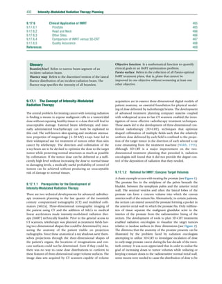
Figure 18 The leaf aperture sequence produced by the matrix method. The MU identify the order of the sequence. The leaf-track numbers are
given to the right of each instance of the sequence. Note that the gaps sweep from right to left. The sequence of gap widths and locations are the same as
that depicted for the step-and-shoot sequence given in Figure 16.

divisions of labor. Initially, the installation of the system must
be probed with extensive tests and measurements to demon-
strate acceptable performance and to collect, verify, and install
data for the computer files that will be used routinely. These
tests then evolve into efficient routine tests intended to verify
that the system continues to perform as initially demonstrated.
The IMRT system is extensive, overlapping with more routine
treatment procedures and processes, consisting of
• the general imaging equipment (CT scanners, MRI
scanners, PET/CT scanners, and gamma cameras) used to
Position (cm)
AccumulatedMU
Leaf position schedule
Leaf A
Leaf B
0.0-1.0-2.0-3.0-4.0-5.0-6.0
0
10
20
30
40
50
60
70
80
90
100
1.0 2.0 3.0 4.0 5.0 6.0
Figure 20 Computed leaf trajectories for the fluence profile in Figure 19. The schedules for leaf A and leaf B are a function of total time that is in
turn proportional to MU. Leaf B begins moving with maximum velocity (red line), while leaf B produces the beam modulation. Then, the roles are
switched back and forth in each gradient region for the rest of the sequence.
Position (cm)(a)
FluenceF
Position (cm)(b)
FluenceF
Position (cm)(c)
FluenceF
Position (cm)
1/Vmax
(d)
FluenceF
Figure 19 Graphic description of the derivation of the dynamic MLC (DMLC) algorithm. Panel (a) depicts the fluence profile to be delivered and
indicates the positive and negative gradient regions. Panel (b) depicts a rotation of the negative gradient regions about the horizontal. Panel (c) depicts a
shift of the regions to remove discontinuities in a leaf opening window. Panel (d) depicts the shear of the trajectories to account for the maximum
leaf speed.

acquire the volumetric studies required for treatment
planning;
• the treatment planning systems (high-end graphic worksta-
tions, a computer network, servers, and associated network
and treatment planning software and files) used to produce
the three-dimensional dose model, the treatment delivery
files, and the position verification digitally reconstructed
radiographs (DRRs) and to generate reports and records
for documentation and billing;
• the medical linear accelerators with their accouterments
(MLC, custom positioning gadgets, optical localization
cameras, and associated software and files);
• treatment imaging devices (EPID, ultrasonic system, fixed
x-ray sources and detector panels, and their associated soft-
ware and files);
• special-purpose instrumentation (automated water-
phantom scanners with high-resolution ionization cham-
bers and diodes with required electronics, software, and
interfaces; static quality assurance phantoms for imaging
and mechanical position measurements; phantoms con-
taining detector arrays and their associated electronics,
computer interfaces, and software; film dosimetry systems
with associated scanners and software; and microdosimetry
systems such as stimulated luminescent chips).
The staff must be trained to use this technical panoply of
instruments and software, and critical parameters throughout
the system must be determined, set in appropriate files, and
scheduled for rechecking during ongoing routine quality-
assurance procedures (Ezzell et al., 2003; Low et al., 2011;
Siochi et al., 2009). A critical test sequence is an end-to-end
measurement by which, after all data are acquired and
entered as required in the IMRT system, a simple but typical
treatment volume is devised from the CT scan of a test
phantom, a plan is computed to irradiate the volume, and
measurements are made of the dose delivered by the plan
using instruments embedded in the test phantom (Ezzell
et al., 2009).
9.17.3.3 Dosimetry of the End of the Leaf
The electromechanical modulation of x-ray treatment beams
by the gaps between pairs of MLC leaves depends critically on
the physics and technology of creating and controlling the
gaps. The current state of the technology is strongly influenced
by the decision of the majority of vendors to implement MLC
leaves that move perpendicular to the center of the x-ray field
whose leaf ends are curved. This design, although it avoids a
number of design and manufacturing problems, introduces
several implementation problems that affect the dosimetry
of the end of the leaf. Firstly, the effective point of the
leaf-end shadow is nonlinearly related to the position of the
leaf. In addition, the effective x-ray edge is offset from the leaf
shadow away from the radiation field. These problems are
addressed within the control software and treatment planning
software.
The background of the dosimetry of the leaf end will be
developed with the aid of Figure 21. The curved MLC leaf end
has a radius of curvature R. This figure describes the geometry
of a leaf retracted a distance W0
/2, as measured from the center
of the field along the direction of travel of the leaf. The line of
travel of the point a0
on the leaf tip is physically a distance SCD
from the x-ray source. The point a0
projects to a in the plane
passing through the medical linear accelerator isocenter at a
distance SAD from the x-ray source. In this plane, the leaf tip
projection to point a is a distance W/2¼(W0
/2)(SAD/SCD)
from the field center. As the leaf moves away from the central
axis, the edge of the shadow b0
on the curved leaf end moves
from a0
down toward the bottom of the leaf. This causes a
nonlinear relation between the encodable distance W0
/2 and
the shadow cast at b0
that forms the edge of the light field. The
edge of the light field is found (Boyer and Li, 1997) to be a
distance x from the field center as measured in the isocenter
plane where
x ¼ W=2ð ÞÁSCD Æ RÁSAD 1ÀSADffiffiffiffi
SA
p
D2
þ W=2ð Þ2

SCD Æ R Wffiffiffiffi
SA
p
D2
þ W=2ð Þ2
A correction, called the leaf position offset (LPO), can
therefore be calculated. LPO¼xÀW0
/2, for a typical MLC
leaf, is shown in Figure 22. This correction is made in the
control software driving the MLC so that the mechanical
leaf-tip position encoding is translated into the position of
the geometric edge of the light field shadow of the leaf in
the isocenter plane. This convention has been used also for
the operation of the MLC controller during IMRT delivery,
even though the LPO correction does not give a leaf position
that corresponds to the true edge of the radiation field.
Although this correction causes the digital displays of the
positions of the MLC leaves to agree with the observed light
field edge, another correction must be made for the small
discrepancy between the light field and the edge of the
radiation field.
R
WЈ/2
aЈ
a
bЈ
b
x
W/2
Figure 21 Geometry of the leaf end. A curved MLC leaf is shown in
two positions. On the left side of the figure, the leaf is retracted from the
central axis a distance W/2 to form a symmetric gap of width W. The end of
the leaf at point a0
is retracted a distance W0
/2 from the central axis as
measured a distance SCD from the x-ray source. The projection of the leaf
end projects to point a at a distance SAD from the x-ray source. The leaf
end at b0
casts a shadow of the curved end that projects to point b.
The distance, x, from the central axis to b can be calculated geometrically.
The correction is made in the digital display of the field size.

The transmission through the leaf end can be estimated
using the attenuation properties of the leaf material, tungsten,
at the x-ray energy employed. An example is given in Figure 23
(Boyer and Li, 1997). As can be inferred from Figure 23, the
transmission through the curved MLC leaves at the ends of the
gap formed by two opposed MLC leaves creates an effective
radiation gap width that is a little larger (a little under 1 mm
at each end) than the width of the gap determined by the edge
of the light field. The overall increase in the gap between two
leaf ends had been called the dosimetric leaf gap (DLG). The
-0.3500
-0.3000
-0.2500
-0.2000
-0.1500
-0.1000
-0.0500
0.0000
-20.0000 -15.0000 -10.0000 -5.0000 0.0000
Leaf tip projection (cm)
Leafpositionoffset(cm)
5.0000 10.0000 15.0000 20.0000
Figure 22 Correction for curved leaf end. The correction known as the leaf position offset (LPO), to projected leaf tip position, W0
/2, to obtain the
location of the light field shadow, x¼W0
/2ÀLPO. Note that using this convention, the LPO is always negative.
0
Distance from light-field edge (mm)
Light-field edge on (0,0)
Light-field edge at (10,10)
About 1.2mm Penumbra
Transmissionratio
0
0.1
0.2
0.3
0.4
0.5
0.6
0.7
0.8
0.9
-1-2-3-4-5 1 2 3 4 5
Figure 23 Calculated transmission through the curved leaf end for a tungsten leaf for 6 MV bremsstrahlung x-rays. The calculation uses a full
three-dimensional model of the leaf end. Calculations are made for the leaf end at two positions: at the center of the treatment field, plotted as (- ♦ -)
light-field edge on (0,0), and at a point off-set from the center of the field as (– □ –) light-field edge at (10,10). The calculation predicts very little
dependence of the shape of the transmission through the leaf end (the penumbra width) on position of the leaf within the radiation field. The calculation
predicts an offset from the light field to the point at which radiation is reduced by one-half (the radiation field offset (RFO)) of about 0.3 mm.
Reproduced from Boyer AL and Li S (1997) Geometric analysis of light-field position of a multileaf collimator with curved ends. Medical Physics 24:
757–762, with permission from Medical Physics Publishing.

distance from the light field edge to the point at which the
radiation field drops to one-half of its value inside the gap has
been called the radiation field offset (RFO). The RFO is deter-
mined by the leaf-end shape, the attenuation of the tungsten
leaf, and a number of other more subtle factors caused by
radiation scatter and electron transport in the rapidly decreas-
ing intensity of the edge of the radiation field. The DLG is
twice the RFO. In Figure 23, the RFO is about 0.3 mm. There
are a number of ways to measure the RFO using a sequence of
leaf motions with radiation. A SMLC technique consists of
exposing an x-ray-sensitive film to leaf sequences consisting
of abutting 2 cm gaps (see Figure 24). If the gaps were placed
such that the gaps abutted at the light field edges with no
space between them, there would be a small overdose at the
gap abutments because the radiation through the ends of the
leaves spills over into neighboring gaps. If one places the gaps
with increasing increments of space between the 2 cm gaps
(i.e., space between the light field edges), the overdose will
decrease and eventually become an underdose. One can
determine the offset that produces the smoothest transition
between abutting gaps by exposing a film to a series of gaps
separated by different spaces. For example, one may place a
series of 2 cm gaps abutting with no space between them
along the track of a pair of leaves. In the adjacent MLC leaf
track, one may place a second series of 1.98 cm gaps with,
say, 0.2 mm spaces between them. The penumbra at the edge
of the fields is not Gaussian in shape, so one never achieves a
perfectly smooth transition. The basic idea behind a step-
and-shoot leaf sequence for creating such a film is shown
in Figure 24. In this figure, only two test RFO values are
indicated. A practical sequence would contain ten or more
test values each created on a different leaf track. Such a
film image is given in Figure 25. It was created by exposing
a computerized radiography cassette to a composite step-
and-shoot sequence using 40 MLC leaves of 0.5 mm width.
Nominal 2 cm long gaps were abutted, separated by spaces,
and overlapped. The RFO is one-half the space between the
light field edges that produces the smoothest transition. The
RFO tested along each row is given in the scale to the right of
the image. In this case, the optimal RFO was determined to
be 0.3 mm.
The RFO is a more serious problem for DMLC dosimetry
(Chui et al., 1996). Since the dose to a beamlet is proportional
to the opening and closing time created by the leading and
trailing leaves, a 2 mm error in the calculation of the edge of a
2 cm gap could lead to a 10% error. The smaller the gap, the
greater the relative error. A film measurement of a DMLC
sequence can be used analogous to the SMLC technique
described earlier. An illustrative partial leaf schedule motion is
described in Figure 26. A sequence of films are exposed with the
leading leaf overshooting a nominal control point by increasing
increments corresponding the RFOs, while the trailing leaf
stops ahead of the nominal control point with the same incre-
ments. Figure 27 shows the superposition of two dose profiles
along the dynamic leaf trajectories with an RFO that is too small
and an ideal RFO.
Several other dosimetric features that do not significantly
affect accuracy of delivery have nevertheless been given consid-
erable attention in the literature. An occasional narrow line of
decreased dose can be observed along the sides of the leaf tracks.
The sides of the leaves are shaped to have tongues running
along their lengths that fit into grooves on their neighbors (see
Figure 4). These random narrow dose deficits are due to certain
combinations of placement of neighboring gaps placing the
tongue into the gap. Although they can be observed on films
acquired at the surface of a phantom recording an entire leaf
sequence, the general opinion is that they occur infrequently
and are blurred out by patient motion and electron transport at
depth. Another observable is a slight underdose at the end of a
delivery sequence. This discrepancy is due to the cycle time of the
dose control system that is continually acquiring a digital reading
of the dose delivered from the transmission ion chamber and
processing it with information about the leaf positions to provide
monitoring of the progress of the treatment. There is a random
difference between the instance the treatment first begins and the
instance this feedback sequence begins. If the phase difference
happens to be at its maximum, the beam will be terminated on
themeasurement of total MU delivered independentlyof thetotal
of the dose increments being monitored by the MLC sequence
monitor. The phenomena are measureable at the highest set
dose rates. It becomes essentially invisible at lower dose rates
and is a negligible fraction of the prescribed dose in any event.
0
Position (cm)
Horizontal (Value) Axis Major Gridlines
MU
0
5
10
15
20
25
30
35
40
45
-1-2-3-4-5 1 2 3 4 5
Figure 24 Depiction of step-and-shoot leaf trajectories used for film dosimetry measurement of the RFO. Approximately 2 cm gaps between leaf ends
are produced so that spaces of decreasing width are left around the nominal gap junctions.

9.17.3.4 Practical Dosimetry Considerations
Besides the extensive fundamental depth dose and output
factor data for a treatment beam of a given energy, two param-
eters stand out as critical to the accuracy of the IMRT delivery:
the transmission factor for the MLC leaves and the DLG. The
modulated fields are delivered within the perimeter of a fixed
dose frontier. At any given instance, a full dose is delivered
through the open gaps between leaf ends, and a much lower
dose is delivered by x-rays penetrating the shielding MLC leaves
forming the gaps. However, all of the fields within the area
shielded by the block collimators receive this lower level of
dose during the entire delivery sequence. This excess dose is
precalculated by the planning algorithm and subtracted from
the dose required at each point along the leaf-track profiles
before the leaf sequences are composed. The prediction of this
transmitted dose is determined by the MLC leaf transmission
factor. Its accuracy affects the overall agreement between cal-
culated and measured doses in a delivered MLC treatment by
several percent. The value of the DLG affects the agreement
between measured and calculated doses by several percent.
Regions where leaf gaps abut appear randomly throughout
any fixed gantry field. The value selected for the RFO can lead
to strands of overdose or underdose streaming through the
irradiated volume from the directions of the employed fixed
fields leading to a discrepancy between measurements and
calculations. The measurements of end-to-end tests described
earlier can be used to recalculate the associated treatment dose
distributions in order to test small changes in the calculation
accuracy affected by small proposed revisions of the measured
0.20
0.19
0.18
0.17
0.16
0.15
0.14
0.13
0.12
0.11
0.10
0.09
0.08
0.07
0.06
0.05
0.04
0.03
0.02
0.01
-0.01
-0.02
-0.03
-0.04
-0.05
-0.06
-0.07
-0.08
-0.09
-0.10
-0.11
-0.12
-0.13
-0.14
-0.15
-0.16
-0.17
-0.18
-0.19
-0.20
Figure 25 Film dosimetry determination of the RFO for SMLC techniques. 2 cm wide gaps were abutted by a step-and-shoot sequence devised to
produce a 2 mm overlap (RFO¼À2 mm) between light field gaps (top of figure) to 2 mm intergap space (RFO¼þ2 mm) at the bottom of figure
(see Figure 24). The test RFOs are at right in cm. Horizontal lines are drawn over the image to show the tracks of the MLC leaf pairs. Shown here are the
resulting overdose triangles at the top end of the strips and the underdose triangle at the bottom end. The optimal RFO is at the point at which the
tips of these triangles meet. Crosshairs mark the location of the leaf pair with a RFO corresponding to the minimum of a curve fit to the variance of the
gray-scale values in ROIs running along the abutment columns of the gaps. The average value of the RFO optimal by this criterion was 0.03 cm.

leaf transmission factor and RFO. This procedure can lead to a
practical improvement in the overall accuracy of the system.
Care must obviously be taken in selecting the end-to-end tests
to represent the range of clinical conditions that will be
encountered.
9.17.4 Direct Aperture Optimization
The traditional approach to IMRT planning for step-and-
shoot delivery consists of two steps, which we described in
Sections 9.17.2 and 9.14.3. At the first stage, a fluence map
is optimized; at the second stage, the fluence map is converted
into a set of deliverable apertures. This two-step approach has
two main disadvantages:
• An accurate representation of the fluence map may require
a large number of apertures. This is undesired since that
may lead to prolonged treatment times. If the same treat-
ment plan quality can be achieved with a smaller number of
apertures, such a treatment plan will be preferred.
• Sequencing leads to dose discrepancy between the idealized
dose distribution of the fluence map solution and the dose
distribution of the apertures – even if the collection of
apertures represents the fluence map exactly. This is due to
the inherent limitations of the dose-deposition matrix con-
cept, which does not take the impact of the delivery hard-
ware into account.
One approach to mitigate dose discrepancies after
sequencing consists in a regularization of the fluence map
during the FMO step. Nevertheless, it is desirable to directly
optimize the intensities and shapes of the apertures. This
IMRT planning approach has been named direct aperture
optimization (DAO).
One advantage in FMO is that the objective function and its
gradient can be formulated explicitly in terms of the optimiza-
tion variables, that is, the dose distribution is a linear function
of the beamlet weights. In DAO, the situation is more complex,
since the dose distribution is not a simple function of the leaf
positions. In addition, FMO can be formulated as a convex
optimization problem such that established algorithms for
continuous optimization reliably find the optimal solution.
DAO, defined as the problem of finding the best treatment
plan that is achievable with at most K apertures, is a nonconvex
optimization problem. Early work on DAO has therefore used
stochastic search methods. In the original work by Shepard
et al. (2002), simulated annealing has been used.
In this section, two approaches to DAO are discussed. The
first method (Section 9.17.4.1) consists in a local leaf position
optimization (Carlsson, 2008; Cassioli and Unkelbach, 2013)
and is implemented in some of the commercial treatment
planning systems (Hardemark et al., 2003). The second method
(Section 9.17.4.2) generates apertures one after another until
a satisfactory treatment plan is obtained. At each stage, an
aperture is identified that promises a large improvement to the
objective function value (Romeijn et al., 2005).
9.17.4.1 Local Leaf Position Optimization
In this approach to DAO, we assume that we are given an
initial set of apertures. This set of apertures can, for example,
be obtained by sequencing a fluence map solution or from
the column generation method discussed in Section 9.17.4.2.
The set of K apertures, indexed by k, is characterized by
• aperture intensities yk, and
• leaf positions for the left and right leaf edges for every leaf
pair n: Lnk and Rnk.
The goal of gradient-based leaf refinement is to optimize
the objective function f(d) with respect to the leaf positions
Position (mm)
RFO 1
RFO 1
RFO 0
RFO 2
RFO 2
Time(s)
Figure 26 Leaf trajectories to measure RFO for dynamic MLC delivery.
The trajectories around one nominal gap junction are depicted with
two RFO test settings.
0
X (cm)
Pair-1 Pair-2 Pair-3
Effect of rounded leaf-end
Pair-4
Dose(cGy)
−2−4−6
0
10
20
30
40
50
2 4 6
Figure 27 The film measurement of the RFO for a DMLC technique.
The top curve with the overdoses was created using DMLC sliding
windows that followed a trajectory with an RFO that was too small.
The lower curve was created with an RFO that was optimal. Reproduced
from Chui CS, Spirou S, and LoSasso T (1996) Testing of dynamic
multileaf collimation. Medical Physics 23: 635–641, with permission
from Medical Physics Publishing.

and aperture weights. In particular, we allow the leaf positions
to change continuously, that is, the leaf edge does not have to
be positioned at a beamlet boundary. This is schematically
illustrated in Figure 28.
9.17.4.1.1 Approximate dose calculation
In FMO, the dose-deposition matrix concept is used to relate
the dose distribution to the optimization variables (beamlet
intensities). In DAO, the situation is more complex, since the
dose distribution is not a simple function of the optimization
variables (leaf positions). Our first task is therefore to formu-
late approximately the dose distribution as a function of the
optimization variables.
The dose in voxel i is given by the sum of the contributions
of the individual apertures, weighted with their intensity yk.
Furthermore, the dose contribution of each aperture is given by
the contributions Fkn
i
of each leaf pair of the MLC:
di ¼
X
k
X
n
ykFi
kn Lkn; ; Rknð Þ
To proceed, we have to further characterize the function
Fkn
i
(Lkn,Rkn). For that purpose, we consider a particular MLC
row n in aperture k. We first imagine that the left leaf is located
at the left most position at the edge of the field; and we
consider the dose contribution of the MLC row as a function
of the right leaf position, which we denote by function
fkn
i
(Rkn). Let us further assume that the voxel i is within the
beam’s eye view of the MLC row (such that the MLC row
contributes a significant dose to voxel i). We know that the
function fkn
i
(Rkn) has the shape of a smooth step function: if
the right leaf is located at the left most position, the MLC row is
closed and the dose contribution is zero. While the right leaf is
moving to the right, the dose contribution increases monoton-
ically. This is illustrated in Figure 29.
We now consider the dose-deposition matrix representa-
tion of the dose to further characterize the function fkn
i
(Rkn).
We note that we know the function fkn
i
(Rkn) at discrete points,
namely, when the right leaf is positioned at an edge of a
beamlet. Let Dx denote the size of a beamlet, and let j denote
the beamlet index in leaf motion direction. At position jDx, the
dose contribution is simply given by the sum over the exposed
beamlets, that is,
fi
kn Rkn ¼ jDxð Þ ¼
Xj
l¼1
Di
knl
For a continuous leaf position in between, we consider a
linear interpolation (Figure 29). This corresponds to the
assumption that the dose distribution of a beamlet that is
half exposed is given by the beamlet dose distribution with
half the intensity. This approximation will break down for
large beamlet size Dx. However, for practical beamlet sizes of
Leaf pair (n)
Beamlet index ( j)
1
1
2
3
4
5
2 3 4 5
Figure 28 Schematic illustration of direct aperture optimization (DAO)
using local leaf position optimization. In fluence map optimization
(FMO) (left), the intensity of each beamlet is optimized. For DAO (right),
the intensity for all beamlets exposed in the aperture is constant.
Instead, the MLC leaf positions, which define the shape of the aperture,
are optimization variables.
Location of voxel i projected
onto the MLC row
Beamlet j / position
along the MLC row
Dose contribution
Dknj
i
5
j=1
fnk(Rnk)
∑
Dknj
i
4
j=1
∑
4Δx 5Δx
i
Figure 29 Illustration of the function fkn
i
(Rkn), representing the dose contribution of a MLC row to a voxel as a function of the right leaf position.
The function is known at discrete position where the right leaf is positioned at a beamlet boundary and the dose contribution can be expressed as a sum
of dose-deposition matrix elements. In between, the dose contribution is interpolated linearly.

5 mm, the approximation yields adequate results. Using the
function fkn
i
, we can express the dose contribution of an MLC
row as
Fi
kn Lkn; Rknð Þ ¼ fi
kn Rknð Þ À fi
kn Lknð Þ
The first term represents the beamlets that are exposed by
the right leaf, and the second term subtracts the beamlets that
are blocked by the left leaf.
9.17.4.1.2 Optimizing leaf positions
To optimize leaf positions and aperture intensities, we can
utilize gradient descent-based algorithms for nonlinear opti-
mization. To apply the generic gradient descent algorithm
described in Section 9.17.2.4.2, we have to evaluate the gradi-
ent of the objective function with respect to leaf positions and
aperture intensities.
With the help of the function f, we can also approximate
the gradient of the objective function with respect to the leaf
positions. Let us consider the derivative with respect to one of
the right leaves Rkn:
@f
@Rkn
¼
XN
i¼1
@f
@di
@di
@Rkn
¼
XN
i¼1
@f
@di
@fi
kn Rknð Þ
@Rkn
The calculation of the partial derivatives @f/@di is identical
to the case of FMO as described in Section 9.17.2.4.2. Using
the linear approximation illustrated in Figure 29, the derivative
of the dose contribution function fkn
i
(Rkn) only depends on
the beamlet where the leaf edge is currently located. If we
further assume that the leaf position is measured in units of
beamlets (i.e., moving a leaf by the width of one beamlet
corresponds to a distance of 1), the derivative of fkn
i
(Rkn) is
simply given by
@fi
kn Rknð Þ
@Rkn
¼ Di
knj
where j is the index of the beamlet where the leaf edge is
located. The derivative of the voxel dose with respect to the
aperture intensity is simply given by the dose contribution of
the aperture for unit intensity:
@di
@yk
¼
X
n
Fi
kn Lkn; ; Rknð Þ
Evaluating the dose gradient of the objective function
with respect to the optimization variables provides the pre-
requisites for the use of a gradient-based nonlinear optimiza-
tion algorithm. In contrast to the FMO, DAO considers two
types of optimization variables simultaneously, that is, leaf
positions and aperture intensities. Therefore, the use of second
derivatives in the optimization algorithm is important
(Section 9.17.2.4.3). In particular, the quasi-Newton methods
like the L-BFGS can be used.
DAO provides the opportunity to directly account for rest-
rictions of the MLC during optimization. These can be integrated
into the optimization problem in the form of bound constraints
and linear constraints. For example, if an MLC does not allow
for interdigitation, this can be accounted for by adding linear
constraints to the optimization problem. For example, the
constraint Lkn Rk(nþ1) requests that the left leaf of leaf
pair n cannot pass the right leaf of the adjacent leaf pair nþ1.
9.17.4.2 Aperture Generation Methods
Section 9.17.4.1 describes a method to locally refine an initial
set of apertures. An alternative approach to DAO consists in
generating apertures one after another until a satisfactory treat-
ment plan is obtained. Early work in this direction has been
based on geometric considerations, that is, apertures are gen-
erated based on the shape of the target and the OARs in the
beams-eye-view.
In this section, an optimization-based approach to gene-
rating apertures is described, which is referred to as the column
generation approach to DAO. The term column generation
originates from a so-named methodology in optimization
theory. The idea behind this method consist of the following
two steps:
1. In the first step, a promising new aperture is identified,
which is guaranteed to improve the objective function
value. Furthermore, we seek to identify an aperture, which
promises a large improvement in plan quality. In the liter-
ature, this step is referred to as the pricing problem.
2. In the second step, the intensities yk of the existing apertures
are optimized. This step is referred to as the master
problem.
The two steps are iterated until a satisfactory treatment
plan quality is reached or a maximum number of apertures is
generated. The optimization of aperture intensities in the sec-
ond step can utilize gradient-based algorithms as described in
Section 9.17.4.1. Thus, the main novelty in this approach
amounts to the identification of promising new apertures in
step one.
9.17.4.2.1 Generating new apertures
We assume that we are given a current set of apertures and we
want to determine a new aperture to be added to the treatment
plan. Furthermore, we would like to find an aperture that leads
to a large improvement in treatment plan quality. In this
section, we formulate this task mathematically.
Let us consider an objective function f(d). For simplicity,
we assume that there are no dosimetric constraints gk. We
further assume that we have optimized the weights of the
existing apertures and we denote their intensities as yk*. Let
us now consider a candidate aperture Ak, which corresponds
to a set of exposed beamlets. We want to assess whether
adding this aperture to the treatment plan improves its
quality. To that end, we can calculate the gradient of the
objective function with respect to the intensity of the candi-
date aperture:
@f
@yA
¼
X
i
@f
@di
@di
@yA
The derivative of the dose in voxel i with respect to the
candidate aperture weight yA is given by the total dose contri-
bution of the aperture, which can be expressed as a sum over
the exposed beamlets:
@di
@yA
¼
X
jeA
Dij

Thus, by carrying out the summation over the voxels, the
derivative of the objective function can be written as a sum over
the contributions of the beamlets contained in the aperture:
@f
@yA
¼
X
jeA
@f
@xj
The gradient is evaluated at the current treatment plan
where the existing apertures have their optimal weights yk*
and the candidate aperture weight yA is zero. We know that, if
the derivative is negative, adding the aperture with a small
positive weight will decrease the objective function, that is,
yield an improved treatment plan.
Clearly, we are interested in reaching a good treatment plan
while generating only a small number of apertures. Thus, we
want to find an aperture that not only improves the objective
function but also promises a large improvement. Intuitively,
we expect an aperture to yield a large improvement if the
absolute value of the derivative |@f/@yA| is large. Therefore,
the aim is to find the aperture, which minimizes the (negative)
derivative. This optimization problem is referred to as the
pricing problem and can be written as
minimize
A
X
jeA
@f
@xj
Here, we minimize over the set of all possible apertures that
can be delivered using an MLC. Unlike the optimization of
intensities, this represents a discrete optimization problem:
each beamlet is either contained or excluded from the aperture,
and we seek to determine the optimal set of beamlets that form
a deliverable aperture.
9.17.4.2.2 Solving the pricing problem
In order to determine the aperture that optimizes |@f/@yA|, we
first make the following observation: in the absence of any
restrictions on the aperture shape, the ‘ideal’ candidate aper-
ture simply consists of all beamlets for which the derivative @f/
@xj is negative. Thus, the main difficulty in solving the pricing
problem amounts to finding the closest deliverable aperture
(Brahme, 1988b).
In order to be deliverable, the minimum requirement for all
MLCs is that all exposed beamlets for one leaf pair have to be
consecutive, that is, there cannot be a closed beamlet in
between two open beamlets. This is illustrated in Figure 30.
To determine the optimal aperture that fulfills the consecutive-
ness constraint, we note that the problem can be decoupled
regarding the leaf pairs. We can determine the optimal leaf
opening for each leaf pair separately. To that end, we further
note that the number of possible leaf configurations is in the
order of J2
, where J is the number of beamlets per leaf pair.
Thus, determining the optimal leaf configuration is a compu-
tationally inexpensive problem that can be solved simply by
enumerating all possibilities.
The solution to the pricing problem can be extended to
include additional MLC constraint, for example, interdigita-
tion. In this case, the leaf pairs are no longer independent
because the interdigitation constraint couples two adjacent
leaf pairs. Nevertheless, efficient algorithms exist to solve the
corresponding pricing problem. For the case of interdigitation,
the pricing problem can be formulated as a network flow
problem. The interested reader is referred to the original pub-
lication by Romeijn et al. (2005).
9.17.4.3 Extensions
9.17.4.3.1 Integration of improved dose calculation
Both DAO methods described earlier utilize the dose-
deposition matrix concept for approximating dose calculation,
for approximating gradients, or for generating new apertures.
Thus, the algorithms as described so far improve on the two-
step approach (FMO plus sequencing) regarding the first aspect
described in the beginning of this section: inexact representa-
tion of the FMO solution due to the use of a small number of
apertures. Further extensions of the previously mentioned
algorithms are needed in order to also improve on the second
aspect, that is, inherent limitations in dose calculation accuracy
in the dose-deposition matrix concept. Unlike FMO, DAO
formulations provide the opportunity to do so.
In the column generation approach, the dose-deposition
matrix is used in the pricing problem. The optimization of
aperture intensities in the master problem does not depend
on the dose-deposition matrix, but only on the total dose
distributions of the apertures. Thus, after an aperture is gener-
ated, its true dose contribution can be accurately recalculated
using an advanced and clinically approved dose calculation
algorithm. The optimization of the aperture intensities is
then based on the most accurate and final dose calculation.
MLC row / Leaf pair (n)
Beamlet index ( j)
1
+1
−1
−1
−1 −2
−3 −2
−2−3
+3 −1
−11
2
3
4
5
2 3 4 5
Figure 30 Illustration of the pricing problem in the aperture generation
process. All beamlets for which the derivative is positive are depicted in
gray; numbers represent the value of @f/@xj; green bars indicate the
optimal leaf positions for this example. The ‘ideal’ aperture comprises
of all beamlets for which the partial derivative with respect to the
objective function is negative. However, to form a deliverable aperture,
all exposed beamlets for one leaf pair have to be consecutive. For leaf pair
3, it is better to include the beamlet in column 3 despite its positive
derivative in order to also include the beamlet with negative derivative
in column 4.

In local leaf position optimization, the dose-deposition
matrix can be used to approximate objective function gradients
with respect to leaf positions. However, typically, changes in
the leaf position are relatively small. Thus, one approach to
integrate more accurate dose calculation consists in the follow-
ing idea: at a given iteration of the leaf refinement algorithm,
the dose distributions of the current apertures are calculated
using an accurate dose calculation algorithm. The obtained
dose distributions are taken as a reference. Subsequently, the
dose-deposition matrix is only used to approximate gradients
and small changes to the reference dose distribution, resulting
from small refinements of the leaf position.
9.17.4.3.2 Hybrid methods and extensions
The column generation method represents a greedy technique:
each iteration considers only one aperture to be added. In
practice, it is observed that the column generation method
yields high-quality treatment plans for an acceptable number
of apertures. However, empirically, it suffers from a slow con-
vergence toward the optimal solution. Different approaches
have been proposed to improve on the basic column genera-
tion method.
In the works by Carlsson (2008) and by Cassioli and Unkel-
bach (2013), a hybrid approach is pursued in which the gen-
eration of apertures is combined with gradient-based leaf
position optimization. This can be considered as an extension
of the master problem: instead of only optimizing for the
aperture intensities, the leaf positions are refined, too. This
approach circumvents one of the main problems of the generic
column generation approach as described in Section 9.17.4.2:
it allows changes to existing apertures.
The work by Salari and Romeijn (2012) considers an exten-
sion of the objective function, which reflects the goal of finding
good treatment plans with small number of apertures. A term is
added to the objective function that aims at minimizing the
total number of MU. The latter is simply given by the sum over
all aperture weights. More specifically, the augmented objec-
tive function
wf dð Þ þ 1 À wð Þ
X
k
yk
is considered, where we{0,1} is a weighting parameter that
controls the relative importance of minimizing the total num-
ber of MU. For the special case of a quadratic objective function
f, it is possible to devise an exact algorithm to determine the
optimal treatment plan for a given number of MU.
9.17.4.3.3 Generalization to constrained optimization
By considering an unconstrained optimization problem, we
have taken an intuitive approach to the column generation
approach to DAO. However, the approach can be generalized
to problems including constraints g(d) c. In this case, the
pricing problem can formally be derived from the Karush–
Kuhn–Tucker (KKT) optimality conditions. The derivation
yields an intuitive result: instead of considering the derivative
of the objective function |@f/@yA| in the pricing problem, the
derivative of the Lagrange function is minimized. For further
details, the interested reader is referred to the original publica-
tion by Romeijn et al. (2005).
9.17.5 Multicriteria Planning Methods
IMRT treatment planning has to trade off different, inherently
conflicting, clinical goals. Therefore, IMRT planning represents
a so-called multicriteria optimization problem. The traditional
approach to explore these trade-offs consists in manually
choosing relative weights for different objectives. This can
lead to a time-consuming trail-and-error process.
In this section, we discuss two approaches to address this
challenge. The first approach (Section 9.17.5.1) is referred to
as prioritized optimization (Clark et al., 2008; Wilkens et al.,
2007) or lexicographic ordering (Jee et al., 2007). It is moti-
vated by the assumption that the clinical objectives can be
ranked according to their priority. The second approach
(Section 9.17.5.2), interactive Pareto-surface navigation
methods, aims at developing tools that allow the treatment
planner to interactively explore trade-offs between different
objectives (Craft et al., 2006; Ku¨fer et al., 2003; Monz et al.,
2008). Both approaches are discussed using the example of a
paraspinal tumor geometry introduced in Section 9.17.2.2.
9.17.5.1 Prioritized Optimization
Prioritized optimization assumes that the different planning
objectives can be ranked according to their importance. In the
paraspinal example, let us assume that the treatment planner
sets a constraint on the maximum dose dS
max
in the spinal cord.
The remaining three objectives (for the target, the kidneys, and
the conformity) are ranked. In this case, the highest priority is
given to the target objective; the second priority may be the
sparing of the kidneys; and the third priority is the conformity
of the dose distribution in the remaining healthy tissue.
In the first step of a prioritized optimization scheme, we
obtain the treatment plan that yields the best target dose
homogeneity, irrespective of the two additional planning
goals. To that end, the optimization problem
minimize
1
NT
XNT
i¼1
di À dpres
ð Þ2
subject to di dmax
S for all i E S
is solved. This yields an optimal value f*
T for the quadratic
objective function for the target volume. In the next step, the
target objective is turned into a constraint, while minimizing
the objective with the second highest priority:
minimize
1
NK
XNK
i¼1
di
subject to di dmax
S for all i E S
1
NT
XNT
i¼1
di À dpres
ð Þ2
f*
T þ E
In this formulation, the mean dose delivered to the kidneys
is minimized, subject to the constraint that the target dose
homogeneity deteriorates at most by e compared to the opti-
mally achievable value f*
T. Solving this optimization problem
yields the optimal mean kidney dose f*
K that is achievable
under the given constraints.

In the third and last step, the objective function for dose
conformity is minimized as the only objective, subject to the
constraints that the target and kidney objectives only deterio-
rate by a small e from their optimal value f*
T and f*
K .
Prioritized optimization schemes rely on a clear ranking of
the objectives and make the assumption that higher-ranked
objectives are not compromised to improve lower-ranked
objectives. This is a potential drawback in situations where a
large improvement in one objective can be achieved by only a
minor degradation of a higher-ranked objective.
9.17.5.2 Interactive Pareto-Surface Navigation Methods
The methods described in this section make the assumption
that the treatment planner wants to explore the trade-offs
between different planning goals.
9.17.5.2.1 Pareto optimality
To that end, we first define the concept of Pareto optimality.
A treatment plan is Pareto-optimal if there exists no treat-
ment plan that is at least as good in all objectives and strictly
better in at least one objective.
In other words, it is not possible to improve a Pareto-
optimal treatment plan in one objective without worsening at
least another objective. To illustrate this concept, we consider
the paraspinal example. To that end, we now consider the
maximum spinal cord dose
fS dð Þ ¼ max
iES
dið Þ
as an objective function. And we consider the trade-off
between the target dose homogeneity and the maximum spinal
cord dose. For simplicity, we neglect the kidney and confor-
mity objective for now. By solving a sequence of optimization
problems of the form
minimize
1
NT
XNT
i¼1
di À dpres
ð Þ2
subject to fS dð Þ dmax
S
for different values of dS
max
, we obtain a set of Pareto-optimal
treatment plan. This is illustrated in Figure 31. The set of all
Pareto-optimal treatment plans, that is, all plans that have
optimal target dose homogeneity for a given maximum spinal
cord dose, forms the Pareto surface or Pareto-efficient frontier.
The Pareto surface can be visualized in objective function space
by plotting the optimal tumor objective fT against the corre-
sponding value of the spinal cord maximum dose fS.
For radiotherapy planning, we are interested in choosing a
treatment plan from the Pareto surface. However, it may depend
on the patient’s or physician’s preference which treatment plan to
pick from the Pareto surface. The development of a multicriteria
treatment planning framework has to address two problems:
1. Developing methods to efficiently represent the Pareto sur-
face with a small number of Pareto-optimal treatment plans
2. Providing a graphical user interface and the underlying
mathematical methods that allow the treatment planner
to interactively explore and visualize the trade-offs between
conflicting planning goals
Both tasks appear straightforward in a two-dimensional
trade-off as illustrated in Figure 31. In this case, the Pareto
surface can be approximated with a few treatment plans that
are evenly spaced on the one-dimensional Pareto surface in the
clinically relevant range of spinal cord maximum doses. The
treatment planner can then choose one of these precomputed
treatments plans. However, IMRT planning typically involves
trade-offs between more than two objectives (say, 5–10). It is
apparent that in higher dimensions, the approximation of the
Pareto surface is more challenging due to the curse of dimen-
sionality. In addition, exploring the trade-off space is
nontrivial.
Dominated plans
(undesirable)
Pareto surface
(set of pareto-optimal plans)
Spinal cord
maximum dose
fs=max(di)
ieS
fT=
i=1
NT
NT
dS
Infeasible
Tumor dose
homogeneity
1 ∑
max
(di- dpres)2
Figure 31 Illustration of the Pareto surface for the trade-off between target dose homogeneity and the spinal cord maximum dose. All treatment plans
below the Pareto surface are impossible to achieve; treatment plans above the Pareto surface are undesirable because they can be improved in one
objective without worsening the second objective. Points on the Pareto surface can be generated using the constrained method, that is, by minimizing
the target objective, subject to different spinal cord dose constraints dS
max
.

9.17.5.2.2 Navigating the Pareto surface
We assume for now that we have a set of Pareto-optimal
treatment plans that approximate the Pareto surface. Methods
to generate such plans are outlined in the succeeding text in
Section 9.17.5.2.3. The set of plans forms a database of opti-
mized IMRT plans; each plan is therefore referred to as a
database plan. Given a set of Pareto-optimal database plans,
the planner is to be provided with methods to explore the
trade-off space. A naive way to approach this consists in letting
the treatment planner choose one of the database plans. How-
ever, it is desirable to explore trade-offs in a continuous fash-
ion. To that end, not only database plans themselves are
considered but also their combinations.
9.17.5.2.2.1 Convex combinations of database plans
We assume that a treatment plan is defined through the fluence
map x. Given two treatment plans with fluence maps x1
and x2
,
we can form a convex combination of the two treatment plans
by considering the averaged fluence map
x ¼ q x1
þ 1 À qð Þx2
which is obtained by averaging the beamlet intensities beamlet
by beamlet, using a mixing parameter qE[0,1]. If x1
and x2
are
Pareto-optimal treatment plans, the convex combination of
two plans is expected to be also a ‘good’ treatment plan.
Since the dose distribution is a linear function of the fluence
map, averaging of the fluence maps corresponds to averaging
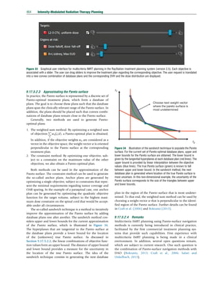
the dose distributions of the two plans. To characterize the
quality of the averaged treatment plan, we discuss its location
in objective space with respect to the Pareto surface. This is
illustrated in Figure 32: by averaging the objective function
values obtained for the two plans, we obtain points
qfT x1
À Á
þ 1 À qð Þ fT x2
À Á
, qfS x1
À Á
þ 1 À qð Þ fS x2
À ÁÀ
in the two-dimensional objective function space. These points
form a line that connects the two Pareto-optimal treatment
plans (red line in Figure 32). For convex objective functions
fT and fS (which is the case for the commonly used functions
except for DVH objectives), it is known (by definition of a
convex function) that the objective functions evaluated at the
averaged fluence map are smaller than the averages of the
objective values, that is,
fT x1
þ 1 À qð Þx2
À Á
q fT x1
À Á
þ 1 À qð Þ fT x2
À Á
and analogously for the spinal cord. On the other hand, the
average treatment plan is not generally Pareto-optimal. There-
fore, the averaged treatment plan is located in between the true
Pareto surface and the linear approximation (red line), as
indicated by the green dot in Figure 32. Informally speaking,
a convex combination of two treatment plans is expected to be
close to being Pareto-optimal if the Pareto surface is relatively
flat in between the plans being averaged. This idea is reflected
in some of the methods to approximate Pareto surfaces using
as small number of plans, for example, the Sandwich method
discussed in the succeeding text.
For real-world IMRT planning problems, more than two
treatment plans can be combined. If there are M database
plans, the exploration of trade-offs can consider the convex
hull of database plans:
x j x ¼
XM
m¼1
qmxm
,
XM
m¼1
qm ¼ 1
( )
9.17.5.2.2.2 Graphical user interface
In a treatment planning system, the planner has to be provided
with tools to navigate in the convex hull of database plans. In a
practical scenario, the planner may have evaluated a current
treatment plan and would like to improve the treatment plan
regarding one particular objective, say, the mean kidney dose.
The treatment planning system has to provide a user interface
to express this request. Figure 33 shows the multicriteria plan-
ning interface in the RayStation treatment planning system,
distributed by RaySearch Laboratories. Each objective is asso-
ciated with a slider. By moving the slider, the user can request
an improvement of the treatment plan with respect to the
corresponding objective. In the background, the treatment
planning system translates the slider movement into a new
convex combination of database plans (Monz et al., 2008).
Qualitatively, a database plan m that was generated by empha-
sizing the objective corresponding to the slider will be assigned
a higher coefficient qm.
For a high-dimensional trade-off space with many objec-
tives, there may be many ways to achieve this goal. For exam-
ple, reducing the dose to the kidneys can be achieved by
compromising target dose homogeneity or by compromising
the conformity of the dose distribution in the remaining nor-
mal tissue. By locking sliders (visible as the check boxes to the
left of each slider in Figure 33), the user has additional control
over the navigation process. For example, by locking the slider
for target dose homogeneity, the user can request that the
navigation is restricted to treatment plans for which the target
homogeneity is no worse than indicated by the current slider
position.
Convex objectives:
True pareto surface
fT
fT (x1
)
fT (x2)
x2
x1
qfT(x1
) +(1−q)fT(x2
)
≥ fT (qx1
+(1−q)x2
)
fS (x2) fSfS (x1)
Figure 32 Illustration of the convex combination of two treatment
plans: treatment plans, defined via the fluence maps x1
and x2
,
correspond to points in the two-dimensional objective function space
spanned by the target and spinal cord objectives fT and fS. For convex
objective functions, an averaged plan is located between the linear
approximation (red line) and the true Pareto surface as indicated by the
green dot.

9.17.5.2.3 Approximating the Pareto surface
In practice, the Pareto surface is represented by a discrete set of
Pareto-optimal treatment plans, which form a database of
plans. The goal is to choose these plans such that the database
plans span the clinically relevant range of the Pareto surface. In
addition, the plans should be placed such that convex combi-
nations of database plans remain close to the Pareto surface.
Generally, two methods are used to generate Pareto-
optimal plans:
1. The weighted sum method: By optimizing a weighted sum
of objectives
P
n
wnfn dð Þ, a Pareto-optimal plan is obtained.
In addition, if the objective weights wn are considered as a
vector in the objective space, the weight vector w is oriented
perpendicular to the Pareto surface at the corresponding
treatment plan.
2. The constraint method: By optimizing one objective, sub-
ject to a constraint on the maximum value of the other
objectives, we also obtain a Pareto-optimal plan.
Both methods can be used in the approximation of the
Pareto surface. The constraint method can be used to generate
the so-called anchor plans. Anchor plans are generated by
optimizing a single objective, subject to constraints that repre-
sent the minimal requirements regarding tumor coverage and
OAR sparing. In the example of a paraspinal case, one anchor
plan can be generated by optimizing the quadratic objective
function for the target volume, subject to the highest maxi-
mum dose constraint on the spinal cord that would be accept-
able under all circumstances.
The so-called sandwich technique is a method to iteratively
improve the approximation of the Pareto surface by adding
database plans one after another. The sandwich method con-
siders upper and lower bounds for the current approximation
of the Pareto surface, which is illustrated in Figure 34.
The hyperplanes that are tangential to the Pareto surface at
the database plans provide a lower bound for the location
of the (unknown) true Pareto surface. As discussed in
Section 9.17.5.2.2, the linear combinations of objective func-
tion values form an upper bound. The distance of upper bound
and lower bound provides a measure for the uncertainty in
the location of the true Pareto surface. The idea of the
sandwich technique consists in generating the next database
plan in the region of the Pareto surface that is most undeter-
mined. To that end, the weighted sum method can be used by
choosing a weight vector w that is perpendicular to the identi-
fied region of the Pareto surface. Further details can be found
in Craft et al. (2006) and Bokrantz (2013).
9.17.5.2.4 Remarks
Multicriteria IMRT planning using Pareto-surface navigation
methods is currently being introduced in clinical practice,
facilitated by the first commercial treatment planning sys-
tems that provide such capabilities. First experience with
multicriteria IMRT planning is being made in a clinical
environment. In addition, several open questions remain,
which are subject to current research. One such question is
the combination of Pareto-surface navigation methods with
DAO (Bokrantz, 2013; Craft et al., 2006; Salari and
Unkelbach, 2013).
Figure 33 Graphical user interface for multicriteria IMRT planning in the RayStation treatment planning system (version 2.5). Each objective is
associated with a slider. The user can drag sliders to improve the treatment plan regarding the corresponding objective. The user request is translated
into a new convex combination of database plans and the corresponding DVH and the dose distribution are displayed.
Choose next weight vector
where the pareto surface is
most undetermined
fS
fT
Figure 34 Illustration of the sandwich technique to populate the Pareto
surface. For the current set of Pareto-optimal database plans, upper and
lower bounds for the Pareto surface are obtained. The lower bound is
given by the tangential hyperplanes at each database plan (red lines). The
upper bound is provided by linear interpolation between the objective
values (blue lines). The true Pareto surface (green) is known to fall
between upper and lower bound. In the sandwich method, the next
database plan is generated where location of the true Pareto surface is
most uncertain. In this two-dimensional example, the uncertainty of the
Pareto surface corresponds to the size of the triangles between upper
and lower bounds.

9.17.6 Clinical Application of IMRT
The clinical management of cancer with radiation using IMRT
attends to (1) the treatment of the primary disease and (2) the
treatment of locally involved lymph nodes. In addition, there
is the problem of treating the postoperative tumor bed follow-
ing surgical removal of the original gross tumor mass. The
treatment of the primary site involves the segmentation of the
gross target volume (GTV) and the values of the extension of
the GTV through a clinical target volume (CTV) and as needed
an internal target volume, to account for respiration, to the
planning target volume (PTV). Anatomical structures to be
spared are segmented as planning risk volumes (PRVs) to
which dose is to be limited (ICRU Report 50, 1993; ICRU
Report 62, 1999). The three-dimensional shape and location
of the PTV and PRVs are then used, along with dose constraints
that relate to the degree of conformity of the dose distribution
to the PTV, to compute the fluence to be delivered by a selected
number of fields irradiating the volume from selected
directions.
Because IMRT allows the radiation oncologist to deliver a
three-dimensional mass of radiation within the patient’s body,
the anatomy determining the shape and the location of this
block becomes extremely important. Numerous efforts have
been undertaken to standardize the definitions of both the PTV
for various treatment sites and the PRVs to be considered for
various treatment sites (www.rtog.org). Protocols for selecting
optimal beam strategies, dose constraints, and other parame-
ters of an IMRT plan depend critically on the treatment plan-
ning facilities and the treatment delivery assets.
9.17.6.1 Prostate
Treatment of the node-negative prostate has become a stan-
dard application of IMRT. A typical treatment plan is given in
Figure 35. Nine fields at even 40
increments are directed
toward an isocenter in the prostate PTV. Appropriate con-
straints are placed on the dose to the bladder and rectum.
The majority of the bladder and rectum are protected to
doses below 45 Gy, whereas the prostate PTV is enclosed by
the 70 Gy isodose surface.
The lymph nodes that drain from the prostate follow the
arteries and veins of the pelvis. These vessels tend to run
together from the lower abdomen, each split right and left as
they enter the bony confines of the pelvic girdle, and then split
again anterior and posterior at about the level of the prostate.
The nodes along the posterior course drain the prostate and are
connected by lymphatic vessels to nodes in the pelvis up into
the lower abdomen. The problem with treating these branch-
ing tubular volumes is that they enclose the sensitive bowels.
With IMRT, it is possible to maintain a relatively low dose in
the enclosed interior while treating the nodal chain to a suffi-
cient dose (see Figure 36). Panel (a) depicts an axial plane
above the prostate demonstrating coverage of the lymph nodes
by 80% isodose curves and protection of the bladder and small
bowel by concavities in the PTV to 50%. Panel (b) depicts a
60%
70%
80% 50%
10%
40%90%
N
(a)
N
B
R
SB 30%
20%
R
S
I 40 % 10 %
20 %
30 %
50 %80 %70%
N N
B
P
(b)
SB
60%
L
Figure 36 Isodose curves for an IMRT treatment of the lymph nodes at risk for metastasis from the prostate. Panel (a) depicts an axial plane
passing above the prostate showing the coverage of the lymph nodes (N) along the medial walls of the pelvic bones while avoiding the rectum (R),
bladder (B), and small bowel (SB). Panel (b) depicts a coronal plane through the same dose distribution demonstrating a dose depression in the center
of the PTV that spares the bladder and SB.
B
P R
14Gy
35Gy
45Gy
56Gy
63Gy
70Gy
Figure 35 Sagittal view of a prostate IMRT plan. Planning risk
volumes (PRVs) include the bladder (B) and the rectum (R). The prostate
planning target volume (PTV) (P) is enclosed by a 70 Gy isodose curve
with the exception of the seminal vesicles. Only a small portion of the
anterior wall of the rectum is exposed to a dose above 63 Gy with
the majority of the rectum less than 35 Gy. The majority of the bladder is
exposed to less than 45 Gy.

coronal plane passing through the nodal PTVs and demon-
strating a depression of dose between the nodal PTV columns
to 50%. Lymphatic cells are more radiosensitive than most
other tumor cells so that the dose gradient need not be as great.
9.17.6.2 Head and Neck
Tumors in the lower head and neck present a variety of treat-
ment planning problems associated with normal sensitive
structures such as the spinal cord, the optic nerves, the lacrimal
glands, the parotid glands, the mucosa of the mouth, and the
esophagus. Tumors arise in the paranasal sinuses, the floor of
the mouth, the larynx, the hypopharynx, and the thyroid.
There are lymph node chains in a string of regions draining
these organs and descending down the neck. The resulting PTV
structures can be quite complex in three dimensions as they
wrap around the PRV structures, leaving few directions of
approach by treatment beams that can cover the PTV structures
with adequate doses without compromising the PTV struc-
tures. Thus, IMRT is employed.
An example of an IMRT plan for a nasopharyngeal tumor is
depicted in Figure 37. A squamous cell carcinoma has pre-
sented on the right wall of the nasopharynx. It has extended
across the back of the nasopharynx and is reaching into the left
wall. It has grown posteriorly into the retropharyngeal space
on the right side. This retropharyngeal extension could not
be treated with opposed lateral fields without compromising
the pons and cerebellum. The PTV extends superiorly to just
below the sella turcica. The PTV extends inferiorly across the
oropharynx. This example employs patient positioning strate-
gies and IMRT. In order to keep the patient’s eyes and optic
nerve out of the treatment fields, the patient’s head is tilted
upward. The position is held by a special-purpose plastic
support behind their head and neck and by a thermoplastic
helmet that holds their head against the support. The treatment
isocenter is placed high so that one of the block collimators
protects the optic apparatus. Treating with half of the beam
avoids divergence of the superior margins of the fields into the
eyes and cranial cavity. The treatment consisted of nine IMRT
fields placed at 40
intervals. In panel (a) of Figure 37, one can
appreciate that IMRT has produced a concavity at the poster
margin of the PTV to protect the pons and cerebellum.
The 90% isodose curve encompasses the PTV. The 30% isodose
curve separates the PTV from the pons and cerebellum. In panel
(b), one can appreciate the irregular shaping of the steep
gradient separating the PTV from the posterior PRV structures
along the column of high dose to follow the course of inferior
tumor spread. Anteriorly, 30% isodose line separates the oral
cavity from the PTV.
9.17.6.3 Other Sites
Mesothelioma is an unusual treatment site (Ahamad et al.,
2003). The tumor is an extremely aggressive malignancy with a
2-year survival rate of around 10%. It recurs locally and generally
is fatal by direct extensions from the site of presentation, even
A
90%
70%
(a)
50%
30%
L
P
R A
S
P
I
30
(b)
90
70
50
Figure 37 A nasopharyngeal tumor. The PTV is an irregular volume that covers the right wall of the nasopharynx and extends across the nasopharynx
and into the right retropharyngeal space close to the cerebellum, pons, and spinal cord. The patient’s head is tilted and the isocenter is placed high
so as to avoid the eyes and optic nerve. Panel (a) is an axial plane through the middle of the PTV and panel (b) is a sagittal plane passing through the
isocenter. The PTV, including the retropharyngeal extension, is enclosed by an isodose curve of 90% of dose at isocenter. The pons receives no
more than 30% of the dose and the cerebellum receives even less.

after surgical resection. IMRT has been used in conjunction with
removal of the lung and the tissues that make up the walls of the
pleural cavity, including those over the heart and diaphragm.
Thus, IMRT is to the surgical bed. A dose between 45 and 60 Gy is
prescribed to a CTV defined by surgical clips. Dose constraints
are placed on the contralateral lung, the heart, the contralateral
kidney, the spinal cord, the liver, and the esophagus. If the
treatment site is on the right side, the liver is protected by a
deep concavity protruding up into the CTV. Seven to eight
beam directions are used. Due to mechanical system constraints
on models of MLCs with limited leaf extension out from second-
ary leaf carriages, two or three carriage settings would be needed
to cover the CTV in the anterior/posterior and lateral/medial
directions (Forster et al., 2003). The isodose distributions pro-
duced by inverse planning are shown in Figure 38. The CTV is
enclosed by the 50 Gy isodose surface defining the prescription
for this case. Remarkably, the deep concavity in the inferior
aspect of the CTV is lined by the 30 Gy isodose surface, protecting
the majority of the liver to a lower dose. The delivery of the
treatment is protracted by the requirement for carriage moves
and occupies the better part of an hour.
9.17.6.4 Comparison of IMRT versus 3D-CRT
Clinical trials have been undertaken to compare 3D-CRT with
IMRT. Although they are essential for investigating and under-
standing the relative merits of any two medical interventions,
these trials are expensive and take years to complete and to
analyze the results. Though less conclusive, another approach
is to use mathematical modeling of the response of tissue to
radiation to compute probabilities of tumor control and nor-
mal tissue sparing resulting from computations of IMRT and
3D-CRT dose distributions with a treatment planning com-
puter. The advantage is that one can make mathematical
comparisons of the two types of treatments using the CT
scans of a cohort of patients, whereas it would be impossible
for each patient to receive the two treatments. Luxton et al.
(2004) carried out a study comparing IMRT treatment plans
for the prostate with 3D-CRT plans for 32 patients. They
computed TCP and NTCPs for appropriate endpoints (see
Section 9.17.2.3.2.1). They demonstrated that IMRT provided
higher TCP values for the prostate (primarily by using slightly
larger daily doses). At the same time, IMRT provided lower
NTCP for the rectum (see Figure 39). These advantages of
IMRT have been observed clinically as well. Hancock et al.
(2000) reported a study comparing the toxicity of 25 patients
treated with IMRT to the prostate and regional lymph nodes
with the toxicity of 34 patients treated contemporaneously
with 3D-CRT (see Figure 40). They found that the preponder-
ance of IMRT patients experienced grade 1 toxicities (defined
by the Radiation Therapy Oncology Group or RTOG to be
increased frequency not requiring medication), whereas the
same percentage of patients treated with 3D-CRT experienced
RTOG grade 2 toxicities (e.g., diarrhea requiring parasym-
patholytic drugs, mucous discharge not requiring pads, and/
or rectal/abdominal pain requiring analgesics). A
L
S
(a)
K50Gy
30 Gy
L
K
30Gy
I
50Gy
(b)
Lu
Figure 38 Treatment of mesothelioma with IMRT. Panel (a) depicts a transverse plane low in the treatment fields that crosses the poles of the kidneys and
the inferior margin of the liver. The clinical target volume (CTV) in red is enclosed by a 50 Gy isodose curve, while the liver and spinal cord are beyond
the 30 Gy isodose curve. Panel (b) is a coronal plane depicting the treatment of the surgical cavity by the 50 Gy volume while sparing the lung and kidney
on the opposite side. The liver that is protected by a deep concavity in the CTV and is mostly beyond the 30 Gy isodose surface. Reproduced from
Forster KM, Smythe WR, Starkschall G, et al. (2003) Intensity-modulated radiotherapy following extrapleural pneumonectomy for the treatment of
malignant mesothelioma: Clinical implementation. International Journal of Radiation Oncology Biology Physics 55: 606–616, with permission from Elsevier.

contemporary study by Zelefsky et al. (2000) observed quali-
tatively similar results. These early results demonstrated the
general notion that the use of IMRT can at least reduce toxic-
ities accompanying radiotherapy, whereas questions of
improved local control take many years to answer. Multiple
clinical trials continue to investigate what advantages can be
realized using IMRT and limitations of the technique at a broad
spectrum of clinical sites (Al-Mamgani et al., 2008; Nutting
et al., 2011).
9.17.6.5 Quality Assurance
Having commissioned the IMRT system, one must perform
checks on the treatment for individual patients, and one must
carry out routine quality assurance procedures for the ongoing
integrity of the IMRT system. The payers of IMRT insurance
claims have required that individual measurements of dose be
made for every patient. This has produced a panoply of com-
mercially offered instruments for this purpose. Any attempt to
catalog the current inventory would soon be obsolete. It is not
feasible to make direct measurement inside each patient. Mea-
surements of the transmission through the patient at each
beam direct have been attempted to reconstruct the dose inside
the patient using back-projected ray tracing. However, this is
not a physical measurement of dose. The acceptable procedure
involves making a measurement of dose in a phantom. Simple
cubic plastic phantoms have been employed as have quasi-
anatomical phantoms (see Figure 41). A treatment simulation
is computed using a CT scan of the phantom and the same
treatment sequences that are planned for the patient. Points
within the phantom are selected, preferably in the PTV and in a
critical OAR, and the dose predicted by the treatment planning
software at these points is noted. A measurement is then made
in the phantom with a suitable small-volume ionization cham-
ber or diode with the phantom irradiated from the same com-
puter files that will be used to treat the patient. The reasoning is
2
10−3
10−2
10−1
4 6 8 10 12
Patient number
Rectum: LFI
n =0.12
m =0.15
TD50=80Gy
3D
IMRT
NTCP
14 16 18 20 22
Figure 39 A plot of rectal normal tissue complication probability (NTCP) for 22 patients treated with local field irradiation (LFI) of the prostate
computed from treatment plans comparing 3D-CRT techniques (solid circles) with IMRT techniques (open triangles). The computations that suggest
lower NTCP can be expected using IMRT. Reproduced from Luxton G, Hancock S, and Boyer AL (2004) Dosimetry and radiobiologic model
comparison of IMRT and 3D conformal radiotherapy in treatment of carcinoma of the prostate. International Journal of Radiation Oncology Biology
Physics 59: 267–284, with permission from Elsevier.
0
0
10
20
30
40
50
60
70
80
1 2
Maximum RTOG score
IMRT-prostate and
nodes
3D-prostate and nodes
GU or GI toxicity
P =0.002
3
Figure 40 Clinical toxicity scores as defined by the Radiation Therapy
Oncology Group (RTOG) for the rectum comparing the results of
treatment of the prostate and lymph nodes using IMRT with 3D-CRT. The
preponderance of IMRT patients experienced grade 1 GU or GI toxicity
(e.g., increased frequency not requiring medication), whereas the same
percentage of the 3D-CRT patients experienced grade 2 toxicity (e.g.,
diarrhea requiring parasympatholytic drugs, mucous discharge not
requiring pads, and/or rectal/abdominal pain requiring analgesics).
Courtesy of Steve Hancock, Stanford.

that if the system calculates a dose that agrees with measure-
ments in the phantom, even though it is not the same as a dose
calculated for the patient in the same relative location in space,
then the system will most likely deliver the same dose in the
patient that it has calculated for the patient. Furthermore, if the
measured dose is within a tolerance at a couple of points, the
dose to the patient is likely to be within tolerance throughout
the treatment volume containing many thousands of beamlets.
Many other instruments containing large arrays of detectors
monitored by computer-based systems are available.
References
Ahamad A, Stevens CW, and Smythe WR (2003) Intensity-modulated radiation therapy:
A novel approach to the management of malignant pleural mesothelioma.
International Journal of Radiation Oncology, Biology, and Physics 55: 768–775.
Al-Mamgani A, Heemsbergen WD, Peeters ST, et al. (2008) Role of intensity-modulated
radiotherapy in reducing toxicity in dose escalation for localized prostate cancer.
International Journal of Radiation Oncology, Biology, Physics 73(3): 685–691.
Bertsekas DP (1999) Nonlinear Programming, 2nd ed. Belmont, MA: Athena Scientific.
Bokrantz R (2013) Multicriteria Optimization for Managing Tradeoffs in Radiation
Therapy Treatment Planning. PhD thesis, Department of Mathematics, KTH Royal
Institute of Technology, Stockholm, Sweden.
Bortfeld T (2006) IMRT: A review and preview. Physics in Medicine and Biology
51: R363–R379.
Bortfeld T, Beurkelbach J, Boesecke R, et al. (1990) Methods of image reconstruction
from projections applied to conformation radiotherapy. Physics in Medicine and
Biology 35: 1423–1434.
Bortfeld T, Boyer AL, Schlegel W, et al. (1994) Realization and verification of three
dimensional conformal radiotherapy with modulated fields. International Journal of
Radiation Oncology, Biology, Physics 30: 899–908.
Bortfeld T, Kahler DL, Waldron TJ, et al. (1994) X-ray field compensation with multileaf
collimators. International Journal of Radiation Oncology, Biology, Physics
28: 723–730.
Boyer AL, Biggs P, Galvin JM, et al. (2001) AAPM Report No. 72 Basic applications of
multileaf collimators. Report of Task Group 50. Madison, WI: Medical Physics
Publishing.
Boyer AL, Ezzell GA, and Yu CX (2012) Intensity-modulated radiation therapy.
In: Khan M and Gerbi BJ (eds.) Treatment Planning in Radiation Oncology, 3rd ed.,
pp. 201–228. Philadelphia, PA: Lippincott, Williams Wilkins.
Boyer AL and Li S (1997) Geometric analysis of light-field position of a multileaf
collimator with curved ends. Medical Physics 24: 757–762.
Brahme A (1988a) Optimization of stationary and moving beam radiation therapy
techniques. Radiotherapy and Oncology 12: 120–140.
Brahme A (1988b) Optimal setting of multileaf collimators in stationary beam radiation
therapy. Strahlentherapie 164: 343–350.
Brahme A, Ka¨llman P, and Lind B (1988) Absorbed dose and biological effect planning
in heavy ion therapy. VIIIth ICMP, San Antonio TX, Physics in Medicine and Biology
33(supplement 1): 73.
Brahme A, Roos J-E, and Lax I (1982) Solution of an integral equation encountered in
rotation therapy. Physics in Medicine and Biology 27: 1221–1229.
Carlsson F (2008) Combining segment generation with direct step-and-shoot
optimization in intensity-modulated radiation therapy. Medical Physics
35: 3828–3838.
Cassioli A and Unkelbach J (2013) Aperture shape optimization for IMRT treatment
planning. Physics in Medicine and Biology 58(2): 301–318.
Censor Y, Altschuler MD, and Powlis WD (1988) A computational solution of the
inverse problem in radiation-therapy treatment planning. Applied Mathematics and
Computation 25: 57–87.
Chui CS, Spirou S, and LoSasso T (1996) Testing of dynamic multileaf collimation.
Medical Physics 23: 635–641.
Clark VH, Chen Y, Wilkens J, Alaly JR, Zakaryan K, and Deasy JO (2008) IMRT
treatment planning for prostate cancer using prioritized prescription optimization
and mean-tail-dose functions. Linear Algebra and its Applications 428(5):
1345–1364.
Craft D, Halabi T, Shih HA, and Bortfeld TR (2006) Approximating convex Pareto
surfaces in multiobjective radiotherapy planning. Medical Physics 33(9):
3399–3407.
Dirkx MLP, Heijmen BJM, and Santvoort JPC (1998) Leaf trajectory calculation for
dynamic multileaf collimation to realize optimized fluence profiles. Physics in
Medicine and Biology 43: 1171–1184.
Ehrgott M, Gu¨ler C, Hamacher HW, and Shao L (2010) Mathematical optimization in
intensity-modulated radiation therapy. Annals of Operations Research
175: 309–365.
Ezzell GA, Burmeister JW, and Dogan N (2009) IMRT commissioning: Multiple
institution planning and dosimetry comparisons, a report from AAPM Task Group
119. Medical Physics 36: 5359–5373.
Ezzell GA, Galvin JM, Low D, et al. (2003) Guidance document on delivery, treatment
planning, and clinical implementation of IMRT: Report of the IMRT subcommittee of
the AAPM radiation therapy committee. Medical Physics 30: 2089–2115.
Forster KM, Smythe WR, Starkschall G, et al. (2003) Intensity-modulated radiotherapy
following extrapleural pneumonectomy for the treatment of malignant
mesothelioma: Clinical implementation. International Journal of Radiation
Oncology, Biology, and Physics 55: 606–616.
Hancock SL, Luxton G, Chen Y, et al. (2000) Intensity modulated radiotherapy for
localized or regional treatment of prostatic cancer. Clinical implementation and
improvement in acute tolerance [Abstract]. International Journal of Radiation
Oncology, Biology, Physics 48: 252–253.
Figure 41 CT scan of a quasianatomical phantom overlaid with a computed IMRT dose distribution. The elliptical cylindrical phantom contains a
cylindrical insert that in turn contains a smaller cylindrical insert offset toward its periphery. An ionization chamber is inserted near the periphery of
the smaller tissue equivalent cylinder at point (I). This cylinder rotates within the larger cylinder whose circumference is made visible by air between
it and the rest of the phantom. Scales on the face of the phantom allow the user to rotate the two cylinders to angles that place the ionization chamber at
any x–y coordinate within the red circle whose diameter is 11.2 cm (e.g., the point (m1)). At (m1), the dose computed in the phantom is 204 cGy,
whereas the patient plan is computed using the MU that would deliver 200 cGy. If the quality assurance tolerance is 2%, a measurement between 200
and 208 cGy would allow the plan to be used for treatment. A second measurement is made at (m2) in a region being protected by a waist in the dose
distribution.

Hardemark A, Liander H, Rehbinder H, and Lo¨f J (2003). Direct Machine Parameter
Optimization with RayMachine in Pinnacle. Raysearch Laboratories White Paper.
ICRU Report (1993) Prescribing, recording and reporting photon beam therapy. ICRU
Report 50. Washington, DC: International Commission on Radiation Units and
Measurements.
ICRU Report 62 (1999) Prescribing, recording and reporting photon beam therapy.
Supplement to ICRU Report 50. Washington, DC: International Commission on
Radiation Units and Measurements.
IMRT Therapy Collaborative Working Group (2001) Intensity-modulated radiotherapy:
Current status and issues of interest. International Journal of Radiation Oncology,
Biology, Physics 51: 880–914.
Jee K-W, McShan DL, and Fraass BA (2007) Lexicographic ordering: Intuitive multicriteria
optimization for IMRT. Physics in Medicine and Biology 52: 1845–1861.
Ka¨llman P, Lind BK, and Brahme A (1992) An algorithm for maximizing the probability
of complication free tumour control in radiation therapy. Physics in Medicine and
Biology 37: 871–890.
Ka¨llman PB, Lind A, Eklo¨f A, et al. (1988) Shaping of arbitrary dose distributions by
dynamic multileaf collimation. Physics in Medicine and Biology 33: 1291–1300.
Ku¨fer KH, Scherrer A, Monz M, et al. (2003) Intensity-modulated radiotherapy – A large
scale multi-criteria programming problem. OR Spectrum 25(2): 223–249.
Lind B and Brahme A (1985) Generation of desired dose distributions with scanned
elementary beams by deconvolution methods. In: Proceedings of the VII ICMP.
Espoo, Finland, pp. 953–954.
Lind BK and Brahme A (1987) Optimization of radiation therapy dose distributions
using scanned electron and photon beams and multileaf collimators.
In: Proceedings of the 9th International Conference on the Use of Computers in
Radiation Therapy, pp. 235–239. Amsterdam: Elsevier.
Ling CC, Burman C, Chui CS, et al. (1996) Conformal radiation treatment of prostate
cancer using inversely-planned intensity-modulated photon beams produced with
dynamic multileaf collimation. International Journal of Radiation Oncology, Biology,
Physics 35: 721–730.
LoSasso T, Chiu CS, and Ling CC (1998) Physical and dosimetric aspects of a multileaf
collimation system used in the dynamic mode for implementing intensity modulated
radiotherapy. Medical Physics 25: 1919–1927.
Low DA, Moran JM, Dempsey JF, et al. (2011) Dosimetry tools and techniques for
IMRT. Medical Physics 38: 1313–1338.
Luxton G, Hancock S, and Boyer AL (2004) Dosimetry and radiobiologic model
comparison of IMRT and 3D conformal radiotherapy in treatment of carcinoma of the
prostate. International Journal of Radiation Oncology, Biology, Physics 59: 267–284.
Ma L, Boyer AL, Ma CM, and Xing L (1999) Synchronizing dynamic multileaf
collimators for producing two-dimensional intensity-modulated fields with
minimum beam delivery time. International Journal of Radiation Oncology, Biology,
Physics 44: 1147–1154.
Ma L, Boyer AL, Xing L, and Ma CM (1998) An optimized leaf-setting algorithm for
beam intensity modulation using dynamic multileaf collimators. Physics in
Medicine and Biology 43: 1629–1643.
Monz M, Ku¨fer KH, Bortfeld TR, and Thieke C (2008) Pareto navigation – algorithmic
foundation of interactive multi-criteria IMRT planning. Physics in Medicine and
Biology 53(4): 985–998.
Nocedal J and Wright SJ (2006) Numerical Optimization, 2nd ed. NY, USA: Springer.
Nutting CM, Morden JP, and Harrington KJ (2011) Parotid-sparing intensity modulated
versus conventional radiotherapy in head and neck cancer (PARSPORT): A phase 3
multicentre randomised controlled trial. Lancet Oncology 12: 127–136.
Romeijn HE, Ahuja RK, Dempsey JF, and Kumar A (2005) A column generation
approach to radiation therapy treatment planning using aperture modulation. SIAM
Journal on Optimization 15(3): 838–862.
Romeijn HE, Dempsey JF, and Li JG (2004) A unifying framework for multi-criteria
fluence map optimization models. Physics in Medicine and Biology 49(10):
1991–2013.
Salari E and Romeijn HE (2012) Quantifying the trade-off between IMRT treatment plan
quality and delivery efficiency using direct aperture optimization. INFORMS Journal
on Computing 24(4): 518–533.
Salari E and Unkelbach J (2013) A column-generation based technique for multi-criteria
direct aperture optimization. Physics in Medicine and Biology 58: 621–639.
Shepard DM, Earl MA, Li XA, Naqvi S, and Yu C (2002) Direct aperture optimization: A
turnkey solution for step-and-shoot IMRT. Medical Physics 29(6): 1007–1018.
Siochi A (1999) Minimizing static intensity modulation delivery time using an intensity
solid paradigm. International Journal of Radiation Oncology, Biology, Physics
43: 671–680.
Siochi AR, Balter P, Bloch CD, et al. (2009) Information technology resource management
in radiation oncology. Journal of Applied Clinical Medical Physics 10: 16–35.
Spirou SV and Chui CS (1994) Generation of arbitrary intensity profiles by dynamic
jaws or multileaf collimators. Medical Physics 21: 1031–1041.
Svensson R, Ka¨llman P, and Brahme A (1994) An analytical solution for the dynamic
control of multileaf collimators. Physics in Medicine and Biology 39: 37–61.
Webb S (1989) Optimization of conformal radiotherapy dose distributions by simulated
annealing. Physics in Medicine and Biology 34: 1349–1370.
Webb S (1993) The Physics of Three Dimensional Radiation Therapy: Conformal
Radiotherapy, Radiosurgery and Treatment Planning. Bristol, UK: Institute of
Physics Publishing.
Webb S (1998a) Configuration options for intensity-modulated radiation therapy using
multiple static fields shaped by a multileaf collimator. Physics in Medicine and
Biology 43: 241–260.
Webb S (1998b) Configuration options for intensity-modulated radiation therapy using
multiple static fields shaped by a multileaf collimator, II: Constraints and limitations
on 2D modulation. Physics in Medicine and Biology 43: 1481–1495.
Webb S (2001) Intensity-Modulated Radiation Therapy. Bristol: Institute of Physics
Publishing.
Webb S (2003) Historical perspective on IMRT. In: Palta JR and Mackie TR (eds.)
Intensity-Modulated Radiation Therapy—The State of the Art, pp. 1–23. Madison,
WI: Medical Physics Publishing.
Wilkens JJ, Alaly JR, Zakarian K, Thorstad WL, and Deasy JO (2007) IMRT treatment
planning based on prioritizing prescription goals. Physics in Medicine and Biology
52: 1675–1692.
Xia P and Verhey LJ (1998) Multileaf collimator leaf sequencing algorithm for
intensity modulated beams with multiple static segments. Medical Physics
25: 1424–1434.
Xing L, Curran B, Hill R, et al. (1999) Dosimetric verification of a commercial inverse
treatment planning system. Physics in Medicine and Biology 44: 463–478.
Xing L, Wu Q, Yong Y, and Boyer AL (2005) Physics of IMRT and inverse treatment
planning. In: Mundt AF and Roeske JC (eds.) Intensity Modulated Radiation
Therapy: A Clinical Perspective, pp. 20–51. Hamilton, Canada: BC Decker Inc.
Publisher.
Zelefsky MJ, Fuks Z, Happersett L, et al. (2000) Clinical experience with intensity
modulated radiation therapy (IMRT) in prostate cancer. Radiotherapy Oncology
55: 241–249.

IMRT

More Related Content

What's hot

Viewers also liked

Similar to IMRT

IMRT