Downloaded 2,076 times


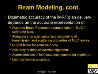


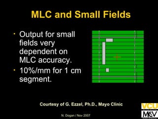
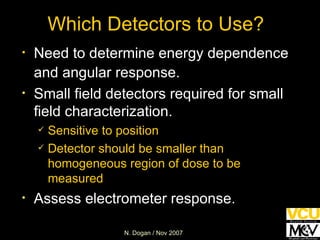
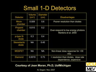
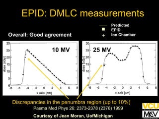


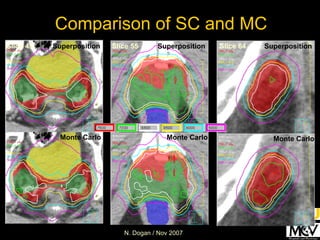

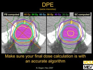
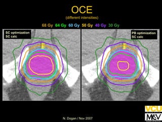
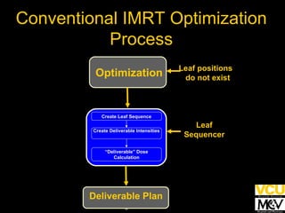

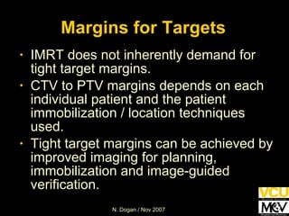
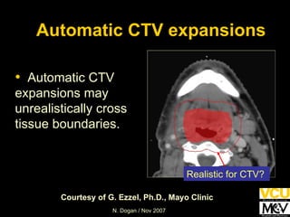

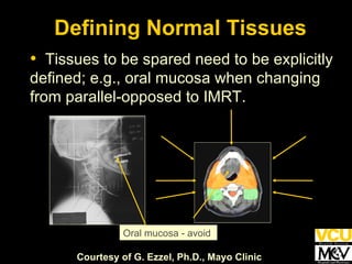
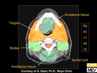


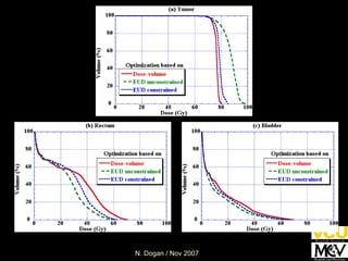
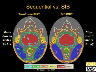


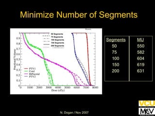
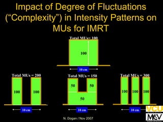

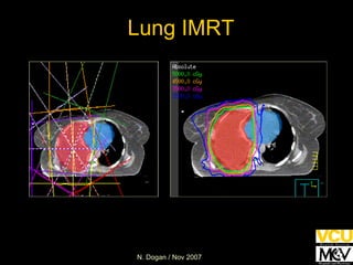
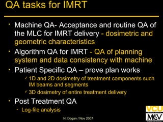


This document summarizes key considerations for intensity-modulated radiation therapy (IMRT) treatment planning and dosimetry. It discusses beam modeling, dose calculation, inverse planning, and quality assurance. Accurate modeling of beam penumbra, multileaf collimator characteristics, output factors for small fields, and dose calculation algorithms are essential for ensuring dosimetric accuracy. Proper target and organ-at-risk delineation and appropriate margins are also important for effective IMRT planning.


![Arc therapy [autosaved] [autosaved]](https://cdn.slidesharecdn.com/ss_thumbnails/arctherapyautosavedautosaved-150423125828-conversion-gate01-thumbnail.jpg?width=640&height=640&fit=bounds)


![CTEV [ clubfoot] DR ARUN LAL ,DR MOHAMED ASHRAF travancore medical college k...](https://cdn.slidesharecdn.com/ss_thumbnails/ctevclubfootdrarunlaldrmohamedashraftravancoremedicalcollegekollamkeralaindia-260208063247-18fc466c-thumbnail.jpg?width=640&height=640&fit=bounds)


![ONFH[AVN HIP] -TRIPLE REGIME -A NOVAL SURGICAL CONCEPT .pptx](https://cdn.slidesharecdn.com/ss_thumbnails/onfhavnhip2026koaconcalicutdrgokuldevdrmashraf-260210064517-213ec005-thumbnail.jpg?width=640&height=640&fit=bounds)


![PERI-PROSTHETIC FRACTURE NAIL-PLATE CONSTRUCT [NPC].pptx](https://cdn.slidesharecdn.com/ss_thumbnails/drarunkumardrmohamedashrafperiprostheticfrasturenail-plateconstructnpc-260209164459-7e9d15a1-thumbnail.jpg?width=640&height=640&fit=bounds)


