The document provides notes on neural networks and regularization from a data science training course. It discusses issues like overfitting when neural networks have too many hidden layers. Regularization helps address overfitting by adding a penalty term to the cost function for high weights, effectively reducing the impact of weights. This keeps complex models while preventing overfitting. The document also covers activation functions like sigmoid, tanh, and ReLU, noting advantages of tanh and ReLU over sigmoid for addressing vanishing gradients and computational efficiency. Code examples demonstrate applying regularization and comparing models.

1. Neural Networks - Part2
Venkat Reddy

2. Statinfer.com
Data Science Training and R&D
statinfer.com
2
Corporate Training
Classroom Training
Online Training
Contact us
info@statinfer.com
venkat@statinfer.com

3. Note
•This presentation is just my class notes. The course notes for data
science training is written by me, as an aid for myself.
•The best way to treat this is as a high-level summary; the actual
session went more in depth and contained detailed information and
examples
•Most of this material was written as informal notes, not intended for
publication
•Please send questions/comments/corrections to info@statinfer.com
•Please check our website statinfer.com for latest version of this
document
-Venkata Reddy Konasani
(Cofounder statinfer.com)
statinfer.com
3

4. Contents
• Overfitting
• Regularization
• Activation Functions
• Learning Rate
4

5. The problem of Overfitting
5

6. The problem of Overfitting
•Neural networks are very powerful. They have capacity to learn any
type of pattern.
•With high number of hidden layers, we can fit to training data with
any level of non-linearity
•Too many hidden layers might be fitting the model for random pattern
or noise in the data
•Throughout the neural network algorithm we were trying optimise
weights to make the error zero. This might lead to overfitting
6

7. Cost function regularization
7
𝐴𝑐𝑡𝑢𝑎𝑙 𝐶𝑜𝑠𝑡 𝑓𝑢𝑛𝑐𝑡𝑖𝑜𝑛 𝑜𝑟 𝐸𝑟𝑜𝑟 = ෍
𝑖=1
𝑛
𝑦𝑖 − 𝑔 ෍
𝑘=1
𝑚
𝑤 𝑘ℎ 𝑘𝑖
2
𝑁𝑒𝑤 𝑅𝑒𝑔𝑢𝑙𝑎𝑟𝑖𝑧𝑒𝑑 𝑒𝑟𝑟𝑜𝑟 = ෍
𝑖=1
𝑛
𝑦𝑖 − 𝑔 ෍
𝑘=1
𝑚
𝑤 𝑘ℎ 𝑘𝑖
2 +
1
2
𝜆 ෍
𝑖=1
𝑛
𝑤𝑖
2
• Apart from minimising error sum of squares, we are minimising error + weights sum of
squares also
• The second term is imposing a penalty on weights.
• This is known as Regularization – What is Regularization

8. What is Regularization?
•In any model building we try to find weights by minimising the cost
function.
•For example in regression we try to find minimum squared error –Cost
function
•Cost function =σ 𝑦𝑖 − σ 𝛽 𝑘 𝑥 𝑘𝑖
2
•Always trying to minimise the overall cost function might not be a
good idea.
•A really high degree polynomial function will make this cost function
zero. But that will lead to overfitting
8

9. LAB: Higher order polynomial model
•Data: Regular/Reg_Sim_Data1.csv
•Plot the points X vs Y
•Build three regression models m1, m2 and m3 and calculate SSE
• m1: simple linear model – Calculate SSE
• m2: Second order polynomial model – Calculate SSE
• m3: Fifth order polynomial model – Calculate SSE
•Which model is the best based on SSE.
9

10. Code: Higher order polynomial model
10
plot(Reg_Sim_Data1$x, Reg_Sim_Data1$y,lwd=10)

11. Code: Higher order polynomial model
11

12. Reduce Overfitting
• We have two options to reduce overfitting
• Build a simple model. Drop all polynomial terms. – But this might lead to underfitting
• Or keep the complex terms but give them less weightage. This will take care of overfitting
• Instead of minimising SSE alone, minimise both SSE and weights
• The regularization term Imposes some penalty on weights. It impacts the overall
weights and reduces the overfitting
12
𝑁𝑒𝑤 𝐶𝑜𝑠𝑡 𝑓𝑢𝑛𝑐𝑡𝑖𝑜𝑛 = ෍ 𝑦𝑖 − ෍ 𝛽 𝑘 𝑥 𝑘𝑖
2
+
1
2
𝜆 ෍𝛽 𝑘
2

13. Regularization comments
•By adding the regularization term we are avoiding the risk of over
fitting
•Regularization also allows us to have a complex model.
•Regularization is added in final cost function but its final impact is on
weights
•A high value of 𝜆 avoids the overfitting
13
𝑁𝑒𝑤 𝐶𝑜𝑠𝑡 𝑓𝑢𝑛𝑐𝑡𝑖𝑜𝑛 = ෍ 𝑦𝑖 − ෍ 𝛽 𝑘 𝑥 𝑘𝑖
2
+
1
2
𝜆 ෍𝛽 𝑘
2

14. LAB: Regularization
•Build a fifth order polynomial function.
•consider new regularized cost function.
•Recalculate the weights. Build three models
• 𝜆 =0
• 𝜆=1
• 𝜆=10
•Plot the models. Which model is more generalised (less over fitted)
•If you have to choose one model with high degree polynomials what
will be your 𝜆 value?
14

15. Code: Regularization
15
Create independent
variable matrix X
Create Dependent
variable matrix Y

16. Code: Regularization
16
• (XtX)-1 (XtY) is the general.
• But we are solving (XtX+ 𝜆)-1 (XtY)
• This is the result of adding
regularization in the cost function

17. Code: Regularization
17
The new weights will be adjusted based
on 𝜆
Observe that when 𝜆 = 0 the
weights are same as usual
regression model

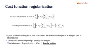
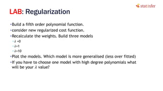
18. Code : Plotting All three models
# plot
plot(mydata,lwd=10)
# lets create many points
nwx = seq(-1, 1, len=50);
x = matrix(c(rep(1,length(nwx)), nwx, nwx^2, nwx^3, nwx^4, nwx^5),
ncol=6)
lines(nwx, x %*% th[,1], col="blue", lty=2)
lines(nwx, x %*% th[,2], col="red", lty=2)
lines(nwx, x %*% th[,3], col="green3", lty=2)
legend("topright", c(expression(lambda==0),
expression(lambda==1),expression(lambda==10)), lty=2,col=c("blue",
"red", "green3"), bty="n")
18

19. Code : Plotting All three models
19
Red line 𝜆=1
Slightly smooth model
Blue line 𝜆=0
Overfitted model when
there is no regularization
Green line 𝜆=10
Very smooth model, almost
a straight line.

20. Code :Choosing the lambda
•If you have to choose one model with high degree polynomials what
will be your 𝜆 value?
20

21. How Regularization works in Neural Nets
•In linear regression having higher order polynomial terms lead to
overfitting.
•Did we reduce the polynomial terms?
•We added regularization term in the cost function recalculated the
weights.
•In neural networks having too many hidden layers might lead to
overfitting.
•Shall we reduce the number of hidden layers?
21

22. How Regularization works in Neural Nets
•In neural network having too many hidden layers will lead to too many
weights, which might lead to over fitting
•Having very less hidden layers might lead to underfitting
•How do we keep several hidden layers with less weightage?
•We can use regularization and have an optimal value for 𝜆 to avoid over
fitting
22
𝐴𝑐𝑡𝑢𝑎𝑙 𝐶𝑜𝑠𝑡 𝑓𝑢𝑛𝑐𝑡𝑖𝑜𝑛 𝑜𝑟 𝐸𝑟𝑜𝑟 = ෍
𝑖=1
𝑛
𝑦𝑖 − 𝑔 ෍
𝑘=1
𝑚
𝑤 𝑘ℎ 𝑘𝑖
2
𝑁𝑒𝑤 𝑅𝑒𝑔𝑢𝑙𝑎𝑟𝑖𝑧𝑒𝑑 𝑒𝑟𝑟𝑜𝑟 = ෍
𝑖=1
𝑛
𝑦𝑖 − 𝑔 ෍
𝑘=1
𝑚
𝑤 𝑘ℎ 𝑘𝑖
2 +
1
2
𝜆 ෍
𝑖=1
𝑛
𝑤𝑖
2

23. Important Note
•We directly work with weights in regularization.
•It is important to standardize the data before applying regularization
in neural networks
•Since a single regularization parameter is applied on all weights, its
very important to bring all weights on to same scale
•Regularization parameter might not have any impact if the data is not
standardised.
23
𝑁𝑒𝑤 𝑅𝑒𝑔𝑢𝑙𝑎𝑟𝑖𝑧𝑒𝑑 𝑒𝑟𝑟𝑜𝑟 = ෍
𝑖=1
𝑛
𝑦𝑖 − 𝑔 ෍
𝑘=1
𝑚
𝑤 𝑘ℎ 𝑘𝑖
2 +
1
2
𝜆 ෍
𝑖=1
𝑛
𝑤𝑖
2

24. Demo: Regularization
24
• Lot of hidden layers
• Overfitted model
• No Regularization
playground.tensorflow.org

25. Demo: Regularization
25
• Lot of hidden layers
Model is not
overfitted
• With Regularization

26. Lab: Regularization in Neural Nets
•Import Credit risk data
•The data has class-imbalance problem. Prepare balance sample for the
model building
•Standardise the data
•Try to build a neural network with 15 hidden nodes
•Set the decay parameter as 0.5
26

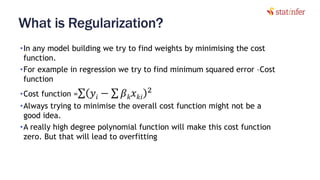
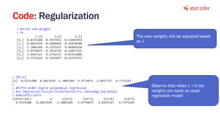
27. Lab: Regularization in Neural Nets
library(clusterSim)
risk_train_strd<-data.Normalization (risk_train[,-1],type="n1",normalization="column")
head(risk_train_strd)
risk_train_strd$SeriousDlqin2yrs<-risk_train$SeriousDlqin2yrs
# x vector, matrix or dataset type ;type of normalization: n0 - without normalization
# n1 - standardization ((x-mean)/sd)
# n2 - positional standardization ((x-median)/mad)
# n3 - unitization ((x-mean)/range)
27
Normalize the data

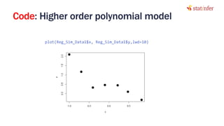
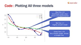
28. Lab: Regularization in Neural Nets
library(nnet)
set.seed(35)
mod1<-nnet(as.factor(SeriousDlqin2yrs)~., data=risk_train,
size=15,
maxit=500)
####Results and Intime validation
actual_values<-risk_train$SeriousDlqin2yrs
Predicted<-predict(mod1, type="class")
cm<-table(actual_values,Predicted)
cm
acc<-(cm[1,1]+cm[2,2])/(cm[1,1]+cm[1,2]+cm[2,1]+cm[2,2])
acc
####Results on test data
actual_values_test<-risk_test$SeriousDlqin2yrs
Predicted_test<-predict(mod1, risk_test[,-1], type="class")
cm_test<-table(actual_values_test,Predicted_test)
cm_test
acc_test<-(cm_test[1,1]+cm_test[2,2])/(cm_test[1,1]+cm_test[1,2]+cm_test[2,1]+cm_test[2,2])
acc_test
28

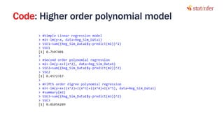
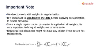
29. Lab: Regularization in Neural Nets
library(nnet)
set.seed(35)
mod1<-nnet(as.factor(SeriousDlqin2yrs)~., data=risk_train,
size=15,
maxit=500,
decay = 0.5)
####Results and Intime validation
actual_values<-risk_train$SeriousDlqin2yrs
Predicted<-predict(mod1, type="class")
cm<-table(actual_values,Predicted)
cm
acc<-(cm[1,1]+cm[2,2])/(cm[1,1]+cm[1,2]+cm[2,1]+cm[2,2])
acc
####Results on test data
actual_values_test<-risk_test$SeriousDlqin2yrs
Predicted_test<-predict(mod1, risk_test[,-1], type="class")
cm_test<-table(actual_values_test,Predicted_test)
cm_test
acc_test<-(cm_test[1,1]+cm_test[2,2])/(cm_test[1,1]+cm_test[1,2]+cm_test[2,1]+cm_test[2,2])
acc_test 29

30. Finetuning neural network
models
30

31. Major Parameters for finetuning NN
•Two major parameters
• Number of hidden nodes/ layers
• The decay parameter
•If number of hidden nodes are high they decay should be high to
regularize.
•If the decay is too high then the model might be underfitted.
•We need to choose an optimal pair of hidden nodes and decay
31

32. Activation Functions
32

33. Activation Functions - Sigmoid
•Sigmoid function. Historically famous
activation function
•Also known as Inverse logistic
•Works well for usual business related a
data
•Works well for a binary or multi class
output
• it takes a real-valued number and
“squashes” and outputs number
between 0 and 1.
•Large negative numbers become 0 and
large positive numbers become 1. 33

34. Sigmoid- Drawbacks
•Sigmoid output not zero-centered.
• The middle value is 0.5
• Most of the times we normalise the data(zero-centered) before building the neural
network model.
•Vanishing Gradients
• Computationally sigmoid values and gradient values and their multiplications are
very small
• For a deep network with many hidden layers sigmoid gradients vanish very quickly
•We need a different activation function which is zero-centered for
better results.
34

35. New Activation Function- TanH
35
• The tanh similar to sigmoid
• Squashes the real values between -1 and +1
• The output is zero centered.
• Preferred activation function for zero centered
(normalized) data.

36. Demo: Sigmoid vs TanH
36
• Sigmoid takes 275
steps

37. Demo: Sigmoid vs TanH
37
• TahH takes less steps

38. Demo: Sigmoid vs TanH
38
• Sigmoid takes 1,604
steps
• Error is still 15%

39. Demo: Sigmoid vs TanH
39
• TanH takes 600
steps
• Error is less than %

40. New Activation Function
•What if the output is either zero or liner
• Customer paid back the loan(zero loss) or loss of
1%,2%,…100%
• Zero intensity(white/no-image) vs pixel intensity
•The above problem is neither classification nor
regression.
• We have a strong liner proton
• We also have a considerable proportion of zeros
•Sigmoid and Tanh can work on this type of data
but computationally very expensive.
• For a deep network of image processing, computation
and execution time is very critical
•We need a Rectified Linear unit type of activation
function
40

41. ReLU - The Rectified Linear Unit
•Very popular activation function in recent
times
•f(x)=max(0,x)
•In other words, the activation is simply
thresholder at zero
•Very fast compared to sigmoid and tanH
•Works very well for a certain class of
problems
•Doesn’t have vanishing gradient problem. It
can be used for modelling real values
41
f(x)=max(0,x)
f(x)=log(1+ex)

42. Demo: ThnH vs ReLu
42
• TanH takes 1,000
steps

43. Demo: ThnH vs ReLU
43
• ReLU takes less
steps

44. Learning rate
44

45. Learning rate
•The weight updating in neural networks
45
𝑊𝑗𝑘 ∶= 𝑊𝑗𝑘 + ∆𝑊𝑗𝑘
𝑤ℎ𝑒𝑟𝑒 ∆𝑊𝑗𝑘 = 𝜂. 𝑦j 𝛿 𝑘
𝑤ℎ𝑒𝑟𝑒 𝜂 is the learning parameter
𝑊𝑗𝑘 ∶= 𝑊𝑗𝑘 + 𝜂. 𝑦j 𝛿 𝑘
•Instead of just updating the weights based on actual calculations, we will
manually setup weight update parameter 𝜂
•This will make the weights move by a factor 𝜂. How fast /slow you want to
move the weights
•Read it as Step-size

46. Learning Rate tuning
•The speed at which the Neural Network arrives to minimum
•If the step-size is too high, the system will either oscillate about the true
solution or it will diverge completely.
•If the step-size is too low, the system will take a long time to converge on
the final solution.
•Generally start with a large value, reduce it gradually.
46

47. Learning Rate is Important
47
• Small learning rate
• Small steps towards
minima
• Has a risk of ending up
in local minima
• Optimal learning rate
• Avoids local minima
• High chance of
ending at global
minima
• For the actual practical problems the error surfaces are very complex
• Learning rate is very important to avoid local minima

48. Demo: Learning rate
48
• High learning rate
• High error

49. Demo: Learning rate
49
• Very low learning rate
• Too many steps
• Takes a lot of time to
converge

50. Demo: Learning rate
50
• Optimal learning rate
• Low error
• Less steps

51. Thank you
51

52. Our Course is Available on Udemy now
52
https://www.udemy.com/machine-learning-made-easy-beginner-to-advance-using-r/

53. Statinfer.com
Data Science Training and R&D
statinfer.com
53
Corporate Training
Classroom Training
Online Training
Contact us
info@statinfer.com
venkat@statinfer.com