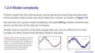
https://youtube.com/OkDevBlog
Deep Learning Foundations and Concepts
1. The Deep Learning Revolution
1.2 A Tutorial Example
https://youtube.com/OkDevBlog
Introduction
For the newcomer to the field of machine learning, many of the basic concepts
and much of the terminology can be introduced in the context of a simple example
involving the fitting of a polynomial to a small synthetic data set.
This is a form of supervised learning problem in which we would like to make a
prediction for a target variable, given the value of an input variable.
https://youtube.com/OkDevBlog
1.2.1 Synthetic data
We denote the input variable by x and the target variable by t, and we assume
that both variables take continuous values on the real axis.
Suppose that we are given a training set comprising N observations of x, written
x1,...,xN, together with corresponding observations of the values of t, denoted
t1,...,tN.
Our goal is to predict the value of t for some new value of x.
The ability to make accurate predictions on previously unseen inputs is a key
goal in machine learning and is known as generalization.
https://youtube.com/OkDevBlog
1.2.1 Synthetic data
We can illustrate this using a synthetic data set generated by sampling from a
sinusoidal function.
Figure 1.4 shows a plot of a training set comprising N = 10 data points in which the
input values were generated by choosing values of xn, for n = 1,...,N, spaced
uniformly in the range [0, 1].
Figure 1.4 Plot of a training data set of N = 10 points, shown as blue
circles, each comprising an observation of the input variable x along
with the corresponding target variable t. The green curve shows the
function sin(2πx) used to generate the data. Our goal is to predict
the value of t for some new value of x, without knowledge of the
green curve.
https://youtube.com/OkDevBlog
1.2.1 Synthetic data
The associated target data values were obtained by first computing the values of
the function sin(2πx) for each value of x and then adding a small level of random
noise (governed by a Gaussian distribution) to each such point to obtain the
corresponding target value tn.
By generating data in this way, we are capturing an important property of many
real-world data sets, namely that they possess an underlying regularity, which we
wish to learn, but that individual observations are corrupted by random noise.
https://youtube.com/OkDevBlog
1.2.2 Linear models
Our goal is to exploit this training set to predict the value of the target variable for some
new value of the input variable.
As we will see later, this involves implicitly trying to discover the underlying function
sin(2πx).
This is intrinsically a difficult problem as we have to generalize from a finite data set to an
entire function.
Furthermore, the observed data is corrupted with noise, and so for a given there is
uncertainty as to the appropriate value for .
Probability theory provides a framework for expressing such uncertainty in a precise and
quantitative manner, whereas decision theory allows us to exploit this probabilistic
representation to make predictions that are optimal according to appropriate criteria.
https://youtube.com/OkDevBlog
1.2.2 Linear models
To start with, however, we will proceed rather informally and consider a simple approach
based on curve fitting.
In particular, we will fit the data using a polynomial function of the form
where M is the order of the polynomial, and xj
denotes x raised to the power of j.
The polynomial coefficients w0,...,wM are collectively denoted by the vector w.
Note that, although the polynomial function y(x,w) is a nonlinear function of x, it is a linear
function of the coefficients w.
Functions, such as this polynomial, that are linear in the unknown parameters have
important properties, as well as significant limitations, and are called linear models.
https://youtube.com/OkDevBlog
1.2.3 Error function
The values of the coefficients will be determined by fitting the polynomial to the
training data.
This can be done by minimizing an error function that measures the misfit between
the function y(x,w), for any given value of w, and the training set data points.
One simple choice of error function, which is widely used, is the sum of the
squares of the differences between the predictions y(xn,w) for each data point
xn and the corresponding target value tn, given by
https://youtube.com/OkDevBlog
1.2.3 Error function
where the factor of 1/2 is included for later convenience.
We will later derive this error function starting from
probability theory.
Here we simply note that it is a nonnegative quantity that
would be zero if, and only if, the function y(x,w) were to
pass exactly through each training data point.
The geometrical interpretation of the sum-of-squares
error function is illustrated in Figure 1.5.
We can solve the curve fitting problem by choosing the
value of w for which E(w) is as small as possible.
Figure 1.5 The error function
(1.2) corresponds to (one half of)
the sum of the squares of the
displacements (shown by the
vertical green arrows) of each
data point from the function
y(x,w).
https://youtube.com/OkDevBlog
1.2.3 Error function
Because the error function is a quadratic function of the coefficients w, its
derivatives with respect to the coefficients will be linear in the elements of w, and
so the minimization of the error function has a unique solution, denoted by w*,
which can be found in closed form.
The resulting polynomial is given by the function y(x,w*).
https://youtube.com/OkDevBlog
1.2.4 Model complexity
There remains the problem of choosing the order M of the polynomial, and as we
will see this will turn out to be an example of an important concept called model
comparison or model selection.
In Figure 1.6, we show four examples of the results of fitting polynomials having
orders M = 0, 1, 3, and 9 to the data set shown in Figure 1.4.
Figure 1.6 Plots of polynomials having various orders M, shown as red curves, fitted to the data set shown in Figure 1.4 by
minimizing the error function (1.2).
https://youtube.com/OkDevBlog
1.2.4 Model complexity
Notice that the constant (M = 0) and first-order (M = 1) polynomials give poor fits to
the data and consequently poor representations of the function sin(2πx).
The third-order (M = 3) polynomial seems to give the best fit to the function
sin(2πx) of the examples shown in Figure 1.6.
When we go to a much higher order polynomial (M = 9), we obtain an excellent fit to
the training data. In fact, the polynomial passes exactly through each data point and
E(w*) = 0.
However, the fitted curve oscillates wildly and gives a very poor representation of
the function sin(2πx). This latter behaviour is known as over-fitting.
https://youtube.com/OkDevBlog
1.2.4 Model complexity
Our goal is to achieve good generalization by making accurate predictions for new
data.
We can obtain some quantitative insight into the dependence of the generalization
performance on M by considering a separate set of data known as a test set,
comprising 100 data points generated using the same procedure as used to generate
the training set points.
For each value of M, we can evaluate the residual value of E(w*) given by (1.2) for the
training data, and we can also evaluate E(w*) for the test data set. Instead of evaluating
the error function E(w), it is sometimes more convenient to use the root-mean-square
(RMS) error defined by
https://youtube.com/OkDevBlog
1.2.4 Model complexity
Graphs of the training-set and test-set RMS errors are shown,
for various values of M, in Figure 1.7.
The test set error is a measure of how well we are doing in
predicting the values of t for new data observations of x.
Note from Figure 1.7 that small values of M give relatively
large values of the test set error, and this can be attributed to
the fact that the corresponding polynomials are rather
inflexible and are incapable of capturing the oscillations in the
function sin(2πx).
Values of M in the range 3 M 8 give small values for the
test set error, and these also give reasonable representations
of the generating function sin(2πx), as can be seen for M = 3
in Figure 1.6.
Figure 1.7 Graphs of the root-
mean-square error, defined by
(1.3), evaluated on the training set,
and on an independent test set, for
various values of M.
https://youtube.com/OkDevBlog
1.2.4 Model complexity
We can gain some insight into the problem by examining the
values of the coefficients w* obtained from polynomials of
various orders, as shown in Table 1.1.
We see that, as M increases, the magnitude of the coefficients
typically gets larger. In particular for the M = 9 polynomial, the
coefficients have become finely tuned to the data.
They have large positive and negative values so that the
corresponding polynomial function matches each of the data
points exactly, but between data points (particularly near the
ends of the range) the function exhibits the large oscillations
observed in Figure 1.6.
Intuitively, what is happening is that the more flexible
polynomials with larger values of M are increasingly tuned to
the random noise on the target values.
Table 1.1 Table of the coefficients
w* for polynomials of various order.
Observe how the typical magnitude
of the coefficients increases
dramatically as the order of the
polynomial increases.
https://youtube.com/OkDevBlog
1.2.4 Model complexity
Further insight into this phenomenon can be gained by examining the behaviour
of the learned model as the size of the data set is varied, as shown in Figure 1.8.
We see that, for a given model complexity, the over-fitting problem become less
severe as the size of the data set increases.
Another way to say this is that with a larger data set, we can afford to fit a more
complex (in other words more flexible) model to the data.
Figure 1.8 Plots of the solutions obtained
by minimizing the sum-of-squares error
function (1.2) using the M = 9 polynomial
for N = 15 data points (left plot) and N =
100 data points (right plot). We see that
increasing the size of the data set
reduces the over-fitting problem.
https://youtube.com/OkDevBlog
1.2.4 Model complexity
One rough heuristic that is sometimes advocated in classical statistics is that the
number of data points should be no less than some multiple (say 5 or 10) of the
number of learnable parameters in the model.
However, when we discuss deep learning later in this book, we will see that
excellent results can be obtained using models that have significantly more
parameters than the number of training data points.
https://youtube.com/OkDevBlog
1.2.5 Regularization
There is something rather unsatisfying about having to limit the number of parameters in a
model according to the size of the available training set.
It would seem more reasonable to choose the complexity of the model according to the
complexity of the problem being solved.
One technique that is often used to control the overfitting phenomenon, as an alternative to
limiting the number of parameters, is that of regularization, which involves adding a penalty term
to the error function (1.2) to discourage the coefficients from having large magnitudes.
The simplest such penalty term takes the form of the sum of the squares of all of the
coefficients, leading to a modified error function of the form
where , , and the coefficient governs the relative importance of
the regularization term compared with the sum-of-squares error term.
https://youtube.com/OkDevBlog
1.2.5 Regularization
Figure 1.9 shows the results of fitting the polynomial of order M = 9 to the same data set as
before but now using the regularized error function given by (1.4).
We see that, for a value of the over-fitting has been suppressed and we now obtain
a much closer representation of the underlying function sin(2πx).
If, however, we use too large a value for then we again obtain a poor fit, as shown in Figure
1.9 for
Figure 1.9 Plots of M = 9 polynomials fitted to the
data set shown in Figure 1.4 using the regularized
error function (1.4) for two values of the
regularization parameter corresponding to
and The case of no regularizer, i.e.,
corresponding to
is shown at the bottom right of Figure 1.6.
https://youtube.com/OkDevBlog
1.2.5 Regularization
The corresponding coefficients from the fitted polynomials are given in Table 1.2, showing
that regularization has the desired effect of reducing the magnitude of the coefficients.
Table 1.2 Table of the coefficients w* for M = 9
polynomials with various values for the
regularization parameter . Note that
corresponds to a model with no regularization,
i.e., to the graph at the bottom right in Figure
1.6. We see that, as the value of increases,
the magnitude of a typical coefficient gets
smaller.
https://youtube.com/OkDevBlog
1.2.5 Regularization
The impact of the regularization term on the
generalization error can be seen by plotting the value
of the RMS error (1.3) for both training and test sets
against as shown in Figure 1.10.
We see that now controls the effective complexity of
the model and hence determines the degree of over-
fitting. Figure 1.10 Graph of the root-mean-square
error (1.3) versus for the M = 9
polynomial.
https://youtube.com/OkDevBlog
1.2.6 Model selection
The quantity is an example of a hyperparameter whose values are fixed during the
minimization of the error function to determine the model parameters w.
We cannot simply determine the value of by minimizing the error function jointly with
respect to w and since this will lead to and an over-fitted model with small or zero
training error.
Similarly, the order M of the polynomial is a hyperparameter of the model, and simply
optimizing the training set error with respect to M will lead to large values of M and
associated over-fitting.
We therefore need to find a way to determine suitable values for hyperparameters.
https://youtube.com/OkDevBlog
1.2.6 Model selection
The results above suggest a simple way of achieving this, namely by taking the available
data and partitioning it into a training set, used to determine the coefficients w, and a
separate validation set, also called a hold-out set or a development set.
We then select the model having the lowest error on the validation set.
If the model design is iterated many times using a data set of limited size, then some over-
fitting to the validation data can occur, and so it may be necessary to keep aside a third
test set on which the performance of the selected model can finally be evaluated.
For some applications, the supply of data for training and testing will be limited. To build a
good model, we should use as much of the available data as possible for training.
However, if the validation set is too small, it will give a relatively noisy estimate of
predictive performance.
https://youtube.com/OkDevBlog
1.2.6 Model selection
One solution to this dilemma is to use cross-validation,
which is illustrated in Figure 1.11.
This allows a proportion (S−1)/S of the available data to be
used for training while making use of all of the data to
assess performance.
When data is particularly scarce, it may be appropriate to
consider the case S = N, where N is the total number of
data points, which gives the leave-one-out technique.
Figure 1.11 The technique of S-fold cross-
validation, illustrated here for the case of S
= 4, involves taking the available data and
partitioning it into S groups of equal size.
Then S −1 of the groups are used to train a
set of models that are then evaluated on
the remaining group. This procedure is
then repeated for all S possible choices for
the held-out group, indicated here by the
red blocks, and the performance scores
from the S runs are then averaged.
https://youtube.com/OkDevBlog
1.2.6 Model selection
The main drawback of cross-validation is that the number of training runs that must be
performed is increased by a factor of S, and this can prove problematic for models in which
the training is itself computationally expensive.
A further problem with techniques such as cross-validation that use separate data to assess
performance is that we might have multiple complexity hyperparameters for a single model
(for instance, there might be several regularization hyperparameters).
Exploring combinations of settings for such hyperparameters could, in the worst case,
require a number of training runs that is exponential in the number of hyperparameters.
The state of the art in modern machine learning involves extremely large models, trained on
commensurately large data sets.
Consequently, there is limited scope for exploration of hyperparameter settings, and heavy
reliance is placed on experience obtained with smaller models and on heuristics.

1.2 A Tutorial Example - Deep Learning Foundations and Concepts.pptx

  • 1.
    https://youtube.com/OkDevBlog Deep Learning Foundationsand Concepts 1. The Deep Learning Revolution 1.2 A Tutorial Example
  • 2.
    https://youtube.com/OkDevBlog Introduction For the newcomerto the field of machine learning, many of the basic concepts and much of the terminology can be introduced in the context of a simple example involving the fitting of a polynomial to a small synthetic data set. This is a form of supervised learning problem in which we would like to make a prediction for a target variable, given the value of an input variable.
  • 3.
    https://youtube.com/OkDevBlog 1.2.1 Synthetic data Wedenote the input variable by x and the target variable by t, and we assume that both variables take continuous values on the real axis. Suppose that we are given a training set comprising N observations of x, written x1,...,xN, together with corresponding observations of the values of t, denoted t1,...,tN. Our goal is to predict the value of t for some new value of x. The ability to make accurate predictions on previously unseen inputs is a key goal in machine learning and is known as generalization.
  • 4.
    https://youtube.com/OkDevBlog 1.2.1 Synthetic data Wecan illustrate this using a synthetic data set generated by sampling from a sinusoidal function. Figure 1.4 shows a plot of a training set comprising N = 10 data points in which the input values were generated by choosing values of xn, for n = 1,...,N, spaced uniformly in the range [0, 1]. Figure 1.4 Plot of a training data set of N = 10 points, shown as blue circles, each comprising an observation of the input variable x along with the corresponding target variable t. The green curve shows the function sin(2πx) used to generate the data. Our goal is to predict the value of t for some new value of x, without knowledge of the green curve.
  • 5.
    https://youtube.com/OkDevBlog 1.2.1 Synthetic data Theassociated target data values were obtained by first computing the values of the function sin(2πx) for each value of x and then adding a small level of random noise (governed by a Gaussian distribution) to each such point to obtain the corresponding target value tn. By generating data in this way, we are capturing an important property of many real-world data sets, namely that they possess an underlying regularity, which we wish to learn, but that individual observations are corrupted by random noise.
  • 6.
    https://youtube.com/OkDevBlog 1.2.2 Linear models Ourgoal is to exploit this training set to predict the value of the target variable for some new value of the input variable. As we will see later, this involves implicitly trying to discover the underlying function sin(2πx). This is intrinsically a difficult problem as we have to generalize from a finite data set to an entire function. Furthermore, the observed data is corrupted with noise, and so for a given there is uncertainty as to the appropriate value for . Probability theory provides a framework for expressing such uncertainty in a precise and quantitative manner, whereas decision theory allows us to exploit this probabilistic representation to make predictions that are optimal according to appropriate criteria.
  • 7.
    https://youtube.com/OkDevBlog 1.2.2 Linear models Tostart with, however, we will proceed rather informally and consider a simple approach based on curve fitting. In particular, we will fit the data using a polynomial function of the form where M is the order of the polynomial, and xj denotes x raised to the power of j. The polynomial coefficients w0,...,wM are collectively denoted by the vector w. Note that, although the polynomial function y(x,w) is a nonlinear function of x, it is a linear function of the coefficients w. Functions, such as this polynomial, that are linear in the unknown parameters have important properties, as well as significant limitations, and are called linear models.
  • 8.
    https://youtube.com/OkDevBlog 1.2.3 Error function Thevalues of the coefficients will be determined by fitting the polynomial to the training data. This can be done by minimizing an error function that measures the misfit between the function y(x,w), for any given value of w, and the training set data points. One simple choice of error function, which is widely used, is the sum of the squares of the differences between the predictions y(xn,w) for each data point xn and the corresponding target value tn, given by
  • 9.
    https://youtube.com/OkDevBlog 1.2.3 Error function wherethe factor of 1/2 is included for later convenience. We will later derive this error function starting from probability theory. Here we simply note that it is a nonnegative quantity that would be zero if, and only if, the function y(x,w) were to pass exactly through each training data point. The geometrical interpretation of the sum-of-squares error function is illustrated in Figure 1.5. We can solve the curve fitting problem by choosing the value of w for which E(w) is as small as possible. Figure 1.5 The error function (1.2) corresponds to (one half of) the sum of the squares of the displacements (shown by the vertical green arrows) of each data point from the function y(x,w).
  • 10.
    https://youtube.com/OkDevBlog 1.2.3 Error function Becausethe error function is a quadratic function of the coefficients w, its derivatives with respect to the coefficients will be linear in the elements of w, and so the minimization of the error function has a unique solution, denoted by w*, which can be found in closed form. The resulting polynomial is given by the function y(x,w*).
  • 11.
    https://youtube.com/OkDevBlog 1.2.4 Model complexity Thereremains the problem of choosing the order M of the polynomial, and as we will see this will turn out to be an example of an important concept called model comparison or model selection. In Figure 1.6, we show four examples of the results of fitting polynomials having orders M = 0, 1, 3, and 9 to the data set shown in Figure 1.4. Figure 1.6 Plots of polynomials having various orders M, shown as red curves, fitted to the data set shown in Figure 1.4 by minimizing the error function (1.2).
  • 12.
    https://youtube.com/OkDevBlog 1.2.4 Model complexity Noticethat the constant (M = 0) and first-order (M = 1) polynomials give poor fits to the data and consequently poor representations of the function sin(2πx). The third-order (M = 3) polynomial seems to give the best fit to the function sin(2πx) of the examples shown in Figure 1.6. When we go to a much higher order polynomial (M = 9), we obtain an excellent fit to the training data. In fact, the polynomial passes exactly through each data point and E(w*) = 0. However, the fitted curve oscillates wildly and gives a very poor representation of the function sin(2πx). This latter behaviour is known as over-fitting.
  • 13.
    https://youtube.com/OkDevBlog 1.2.4 Model complexity Ourgoal is to achieve good generalization by making accurate predictions for new data. We can obtain some quantitative insight into the dependence of the generalization performance on M by considering a separate set of data known as a test set, comprising 100 data points generated using the same procedure as used to generate the training set points. For each value of M, we can evaluate the residual value of E(w*) given by (1.2) for the training data, and we can also evaluate E(w*) for the test data set. Instead of evaluating the error function E(w), it is sometimes more convenient to use the root-mean-square (RMS) error defined by
  • 14.
    https://youtube.com/OkDevBlog 1.2.4 Model complexity Graphsof the training-set and test-set RMS errors are shown, for various values of M, in Figure 1.7. The test set error is a measure of how well we are doing in predicting the values of t for new data observations of x. Note from Figure 1.7 that small values of M give relatively large values of the test set error, and this can be attributed to the fact that the corresponding polynomials are rather inflexible and are incapable of capturing the oscillations in the function sin(2πx). Values of M in the range 3 M 8 give small values for the test set error, and these also give reasonable representations of the generating function sin(2πx), as can be seen for M = 3 in Figure 1.6. Figure 1.7 Graphs of the root- mean-square error, defined by (1.3), evaluated on the training set, and on an independent test set, for various values of M.
  • 15.
    https://youtube.com/OkDevBlog 1.2.4 Model complexity Wecan gain some insight into the problem by examining the values of the coefficients w* obtained from polynomials of various orders, as shown in Table 1.1. We see that, as M increases, the magnitude of the coefficients typically gets larger. In particular for the M = 9 polynomial, the coefficients have become finely tuned to the data. They have large positive and negative values so that the corresponding polynomial function matches each of the data points exactly, but between data points (particularly near the ends of the range) the function exhibits the large oscillations observed in Figure 1.6. Intuitively, what is happening is that the more flexible polynomials with larger values of M are increasingly tuned to the random noise on the target values. Table 1.1 Table of the coefficients w* for polynomials of various order. Observe how the typical magnitude of the coefficients increases dramatically as the order of the polynomial increases.
  • 16.
    https://youtube.com/OkDevBlog 1.2.4 Model complexity Furtherinsight into this phenomenon can be gained by examining the behaviour of the learned model as the size of the data set is varied, as shown in Figure 1.8. We see that, for a given model complexity, the over-fitting problem become less severe as the size of the data set increases. Another way to say this is that with a larger data set, we can afford to fit a more complex (in other words more flexible) model to the data. Figure 1.8 Plots of the solutions obtained by minimizing the sum-of-squares error function (1.2) using the M = 9 polynomial for N = 15 data points (left plot) and N = 100 data points (right plot). We see that increasing the size of the data set reduces the over-fitting problem.
  • 17.
    https://youtube.com/OkDevBlog 1.2.4 Model complexity Onerough heuristic that is sometimes advocated in classical statistics is that the number of data points should be no less than some multiple (say 5 or 10) of the number of learnable parameters in the model. However, when we discuss deep learning later in this book, we will see that excellent results can be obtained using models that have significantly more parameters than the number of training data points.
  • 18.
    https://youtube.com/OkDevBlog 1.2.5 Regularization There issomething rather unsatisfying about having to limit the number of parameters in a model according to the size of the available training set. It would seem more reasonable to choose the complexity of the model according to the complexity of the problem being solved. One technique that is often used to control the overfitting phenomenon, as an alternative to limiting the number of parameters, is that of regularization, which involves adding a penalty term to the error function (1.2) to discourage the coefficients from having large magnitudes. The simplest such penalty term takes the form of the sum of the squares of all of the coefficients, leading to a modified error function of the form where , , and the coefficient governs the relative importance of the regularization term compared with the sum-of-squares error term.
  • 19.
    https://youtube.com/OkDevBlog 1.2.5 Regularization Figure 1.9shows the results of fitting the polynomial of order M = 9 to the same data set as before but now using the regularized error function given by (1.4). We see that, for a value of the over-fitting has been suppressed and we now obtain a much closer representation of the underlying function sin(2πx). If, however, we use too large a value for then we again obtain a poor fit, as shown in Figure 1.9 for Figure 1.9 Plots of M = 9 polynomials fitted to the data set shown in Figure 1.4 using the regularized error function (1.4) for two values of the regularization parameter corresponding to and The case of no regularizer, i.e., corresponding to is shown at the bottom right of Figure 1.6.
  • 20.
    https://youtube.com/OkDevBlog 1.2.5 Regularization The correspondingcoefficients from the fitted polynomials are given in Table 1.2, showing that regularization has the desired effect of reducing the magnitude of the coefficients. Table 1.2 Table of the coefficients w* for M = 9 polynomials with various values for the regularization parameter . Note that corresponds to a model with no regularization, i.e., to the graph at the bottom right in Figure 1.6. We see that, as the value of increases, the magnitude of a typical coefficient gets smaller.
  • 21.
    https://youtube.com/OkDevBlog 1.2.5 Regularization The impactof the regularization term on the generalization error can be seen by plotting the value of the RMS error (1.3) for both training and test sets against as shown in Figure 1.10. We see that now controls the effective complexity of the model and hence determines the degree of over- fitting. Figure 1.10 Graph of the root-mean-square error (1.3) versus for the M = 9 polynomial.
  • 22.
    https://youtube.com/OkDevBlog 1.2.6 Model selection Thequantity is an example of a hyperparameter whose values are fixed during the minimization of the error function to determine the model parameters w. We cannot simply determine the value of by minimizing the error function jointly with respect to w and since this will lead to and an over-fitted model with small or zero training error. Similarly, the order M of the polynomial is a hyperparameter of the model, and simply optimizing the training set error with respect to M will lead to large values of M and associated over-fitting. We therefore need to find a way to determine suitable values for hyperparameters.
  • 23.
    https://youtube.com/OkDevBlog 1.2.6 Model selection Theresults above suggest a simple way of achieving this, namely by taking the available data and partitioning it into a training set, used to determine the coefficients w, and a separate validation set, also called a hold-out set or a development set. We then select the model having the lowest error on the validation set. If the model design is iterated many times using a data set of limited size, then some over- fitting to the validation data can occur, and so it may be necessary to keep aside a third test set on which the performance of the selected model can finally be evaluated. For some applications, the supply of data for training and testing will be limited. To build a good model, we should use as much of the available data as possible for training. However, if the validation set is too small, it will give a relatively noisy estimate of predictive performance.
  • 24.
    https://youtube.com/OkDevBlog 1.2.6 Model selection Onesolution to this dilemma is to use cross-validation, which is illustrated in Figure 1.11. This allows a proportion (S−1)/S of the available data to be used for training while making use of all of the data to assess performance. When data is particularly scarce, it may be appropriate to consider the case S = N, where N is the total number of data points, which gives the leave-one-out technique. Figure 1.11 The technique of S-fold cross- validation, illustrated here for the case of S = 4, involves taking the available data and partitioning it into S groups of equal size. Then S −1 of the groups are used to train a set of models that are then evaluated on the remaining group. This procedure is then repeated for all S possible choices for the held-out group, indicated here by the red blocks, and the performance scores from the S runs are then averaged.
  • 25.
    https://youtube.com/OkDevBlog 1.2.6 Model selection Themain drawback of cross-validation is that the number of training runs that must be performed is increased by a factor of S, and this can prove problematic for models in which the training is itself computationally expensive. A further problem with techniques such as cross-validation that use separate data to assess performance is that we might have multiple complexity hyperparameters for a single model (for instance, there might be several regularization hyperparameters). Exploring combinations of settings for such hyperparameters could, in the worst case, require a number of training runs that is exponential in the number of hyperparameters. The state of the art in modern machine learning involves extremely large models, trained on commensurately large data sets. Consequently, there is limited scope for exploration of hyperparameter settings, and heavy reliance is placed on experience obtained with smaller models and on heuristics.